HAL Id: hal-01008089
https://hal.archives-ouvertes.fr/hal-01008089
Submitted on 9 May 2018HAL is a multi-disciplinary open access archive for the deposit and dissemination of sci-entific research documents, whether they are pub-lished or not. The documents may come from
L’archive ouverte pluridisciplinaire HAL, est destinée au dépôt et à la diffusion de documents scientifiques de niveau recherche, publiés ou non, émanant des établissements d’enseignement et de
Dynamic slope stability analysis by a reliability-based
approach
Dalia Youssef Abdel Massih, Abdul-Hamid Soubra, Jacques Harb, Mohamed
Rouainia
To cite this version:
Dalia Youssef Abdel Massih, Abdul-Hamid Soubra, Jacques Harb, Mohamed Rouainia. Dynamic slope stability analysis by a reliability-based approach. 5th International Conferences on Recent Advances in Geotechnical Earthquake Engineering and Soil Dynamics, May 2010, San Diego, United States. �hal-01008089�
DYNAMIC SLOPE STABILITY ANALYSIS BY A RELIABILITY-BASED
APPROACH
Dalia S. Youssef Abdel Massih
Researcher, National Council For Scientific Research Bhannes, Lebanon
Abdul-Hamid Soubra
Professor, University of Nantes, Institut de Recherche en Génie Civil et Mécanique, UMR CNRS 6183, Bd. de l’université, BP 152, 44603 Saint-Nazaire cedex, France
Jacques Harb, Associate Professor, Notre Dame University,
Department of Civil and Environmental Engineering, P.O. Box 72, Zouk Mikael, Lebanon.
Mohamed Rouainia
Associate Professor, School of Civil Engineering, University of Newcastle, Newcastle upon Tyne NE1 7RU, UK.
ABSTRACT
The analysis of earth slopes situated in seismic areas has been extensively investigated in literature using deterministic approaches where average values of the input parameters are used and a global safety factor or a permanent displacement at the toe of the slope is calculated. In these approaches, a decoupled analysis is usually performed in which a constant critical seismic acceleration is first calculated based on a pseudo-static representation of earthquake effects. Then, the permanent soil displacement is computed by integration of the real acceleration record above the critical acceleration. A reliability-based approach for the seismic slope analysis is introduced in this paper. This approach is more rational than the traditional deterministic methods since it enables to take into account the inherent uncertainty of the input variables. Furthermore, the deterministic model used in the reliability analysis is based on a rigorous coupled analysis that simultaneously captures the fully non linear response of the soil and history of the real acceleration record. This model is based on numerical simulations using the dynamic option of the finite difference FLAC3D software. The acceleration time history records used in this analysis is the one registered at the Lebanese Geophysical Center of the National Council for Scientific Research. The performance function used in the reliability analysis is defined with respect to the horizontal permanent displacement at the toe of the slope. The random variables considered in the analysis are the cohesion
c
and the shear modulus G of the soil since it was shown that these parameters have the most influence on slope displacements. The Stochastic Response Surface Methodology (SRSM) is utilized for the assessment of the probability distribution of the horizontal permanent displacement at the toe of the slope. The results have shown that the mean value of the permanent displacement is highly influenced by the coefficient of variation of the cohesion, the greater the scatter inc
the higher the horizontal permanent displacement. Based on the probability distribution of the permanent displacement, the failure probability with respect to the exceedance of an allowable maximal permanent displacement was evaluated and discussed. At the end of the paper, a case study of a typical Lebanese slope is presented and analyzed to illustrate this approach.INTRODUCTION
Recent earthquake events in South Lebanon in addition to the accidental topography and heterogeneous Lebanese geology have trigerred this research on the analysis of slopes subjected to seismic loads using a probabilistic approach.
The stability analysis of earth slopes located in seismic areas has been extensively investigated in literature using deterministic approaches. In these methods, average values of the input parameters (angle of internal friction, cohesion, seismic coefficient, etc.) are used and a global safety factor is calculated (Refer for instance Chen & Sawada, 1983; Leshchinsky & San, 1994; You & Michalowski, 1999; Michalowski, 2002, and Loukidis et al., 2003 among others). A reliability-based approach for the slope stability analysis in seismic zones is more rational than the traditional deterministic methods since it takes into account the inherent uncertainty of each input variable. The reliability theory was introduced by several authors in the analysis of slope stability but without taking into consideration the seismic loading (Refer for instance Vanmarcke, 1977; Chowdhury & Xu, 1993; Christian et al., 1994; Low et al., 1998; Husein Malkawi et al., 2000; Auvinet & Gonzales, 2000; El-Ramly et al., 2002; and Sivakumar Babu & Mukesh, 2004 among others). Most of these studies are based on approximate deterministic models as the limit equilibrium method which is founded on a priori assumptions concerning (i) the form of the slip surface and (ii) the normal stress distribution along this surface or the inter-slice forces. The application of the reliability theory in slope stability problems subjected to seismic loadings is much less investigated (Refer for instance Christian & Urzua, 1998; Al-Hamoud & Tahtamoni, 2000, 2002; and Youssef Abdel Massih et al., 2009).
In this paper, a reliability-based analysis of an earth slope situated in a seismic area is performed. The deterministic model used in the reliability analysis is based on a rigorous coupled analysis that simultaneously captures the fully non linear response of the soil and the acceleration time history record. This model is based on numerical simulations using the dynamic
option of the finite difference FLAC3D software. The time
history of acceleration records used in the analysis is the one digitized at the Lebanese Geophysical Center of the National Council for Scientific Research. The random variables considered in the analysis are the cohesion
c
and the shear modulus G of the soil since it was shown that these parameters have the most influence on the slope displacements (Dhakal, 2004). The performance function used in the reliability analysis is defined with respect to the horizontal permanent displacement at the toe of the slope. The Stochastic Response Surface Methodology (SRSM) is utilized for the assessment of the Γfailure probability is evaluated with respect to the exceedanceof an allowable maximun permanent displacement. After a brief description of the concepts underlying the stochastic response surface methodology, the seismic deterministic numerical
modeling of a slope using FLAC3D is described. Then, the
probabilistic numerical results are presented and discussed. A case study of a typical Lebanese slope illustrates this approach at the end of the paper.
STOCHASTIC RESPONSE SURFACE METHODOLOGY The stochastic response surface method (SRSM) is a technique for the reliability analysis of complex systems with low failure probabilities, for which Monte Carlo simulation (MCS) is too computationally expensive and for which other approximate methods (such as FORM) may be inaccurate. It allows one not only to determine the failure probability of a system due to a prescribed load as is the case of the traditional response surface methodology (RSM) (e.g. Youssef Abdel Massih and Soubra, 2008), but also to find the full probability distribution of the system response. Typically, SRSM approximates an analytically-unknown limit state function with a multidimensional chaos polynomial by fitting the polynomial to a number of sampling points. Once the coefficients of the polynomial chaos are determined, the probability distribution of the response can be calculated using the classical and well-known Monte Carlo simulation based on the obtained analytical form of the response. Then, the statistical moments of the response (mean, variance, skewness, kurtosis, etc.) may be computed. Furthermore, the analytical equation of the response may be used to calculate the reliability index and the failure probability using the classical methods such as FORM, Monte Carlo, Importance Sampling, etc. The steps used in SRSM can be summarized as follows:
Step I: Representation of Stochastic Inputs
The first step in the application of the SRSM is the representation of all the model inputs in terms of a set of “standardized random variables”. Normal random variables are selected from a set of independent standard distributed normal random variables,
1,...,M
, where M is the number ofindependent inputs, and each i has zero mean and unit
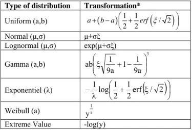
variance. One of two approaches may be taken to represent the uncertain inputs in terms of the selected “standardized random variables”: (a) direct transformation of inputs in terms of the “standardized random variables”, and (b) series approximations in “standardized random variables”. Devroye (1986) presents transformation techniques and approximations for a wide variety of probability distributions of random variables (cf. Table 1)
Table 1 : Representation of common univariate distributions as
function of normal random variables
* y is the exponential (1) distribution Step II: Analytical approximation of outputs
An output of a model (e.g. the permanent displacement at the toe of the slope or the amplification of the slope in the case of the present seismic study) may be influenced by any number of model inputs. Hence, any general functional representation of uncertainty in model outputs, should take into account uncertainties in all inputs. For a deterministic model with random inputs, if the inputs are represented in terms of the set
M1 i i
(as descrribed in step I), the output metrics can also be represented in terms of the same set, as the uncertainty in the outputs is obviously due to the uncertainty of the inputs. The present SRSM method addresses one specific form of representation: the series expansion of normal random variables in terms of Hermite polynomials. The expansion is called “polynomial chaos expansion”. Using this series expansion, an output can be approximated by a polynomial chaos expansion on the set
1 M i i
, given by:
1 1 0 ( ) P ( ) M j j k k j y a
(1)where y is any output metric (or random output) of the model. The aj represent deterministic constants to be estimated,
j aremulti-dimensional Hermite polynomials of order less than or equal to p. They are given by :
e
Te
T ip i p p ip i p 2 1 1 2 1 1...
1
,...,
Γp are random variables since they are functions of the random variables
1n i i
. In equation (1), P denotes the size of the
polynomial chaos basis which is given by:
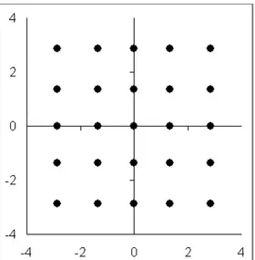
! ! ! M p P M p (2) For a fourth order polynomial and for two random variables, the size of the polynomial chaos basis (which is equal to the number of unknown coefficients) is found to be equal to 15.Step III: Choice of the chaos order and collocation points In general, the accuracy of the approximation increases as the order of the polynomial chaos expansion increases. The order of the expansion can be selected to reflect accuracy needs and computational constraints. After choosing the order of the chaos and the number of the random variables, one can obtain the number of available collocation points and their positions in the standard space of random variables. These points will be used for the evaluation of the system response. In the case of two random variables (as in this paper), the choice of these points is made so that each standard variable (ξ1 or ξ2 in this case) can take the values of the roots of the univariate Hermite polynomial of order n+1. Hence, the available collocation points are obtained by assigning to each root of the first variable the different roots of the second variable.
Table 2 provides the roots and the general shape of the Polynomial Chaos Expansion that will approximate the response of the model (i.e. the toe horizontal permanent displacement or the amplification), for the 4th order of the polynomial chaos (i.e., p = 4). Figure 1 provides the positions of the collocation points (25 points) in the standard space of the random variables.
Table 2 : Roots to be used for the 4th order poynomial chaos and
the expression of the corresponding output.
Type of distribution Transformation*
Uniform (a,b)
1 1
/ 2
2 2 a b a erf Normal (μ,σ) μ+σξ Lognormal (μ,σ) exp(μ+σξ) Gamma (a,b) 3 a 9 1 1 a 9 1 ab Exponentiel (λ)
erf / 2 2 1 2 1 log 1 Weibull (a) a 1 yExtreme Value -log(y)
Roots to be used for the polynomial chaos of
order 4
Expression of the output
0 ; 5 10
4 0,0 0,0 1,0 1,0 1 0,1 0,1 2 2,0 2,0 1 1,1 1,1 1 2 0,2 0,2 2 3,0 3,0 1 2,1 2,1 1 2 1,2 1,2 1 2 0,3 0,3 2 4,0 4,0 1 3,1 3,1 1 2 2,2 ... ... , ... ... , , ... ... , U a a a a a a a a a a a a a 2,2 1 2 1,3 1,3 1 2 0,4 0,4 2 , ... ... a , a Fig. 1: Position of the collocation points in the standard space of the random variables
Translation of the collocation points from the standard to the physical space
For each collocation point
1,m,2,m
, one has to determine thecorresponding physical point
c Gm, m
(i.e the cohesion and theshear modulus) to be used in the deterministic model. If there is a correlation c G, between the random variables cm and Gm, one
should correlate the standard variables by multiplying the vector of standard uncorrelated variables by Cholesky transform H of the standard covariance matrix Σ (obtained from the covariance matrix C) as follows: 1 , 1, 2 , 2, C m m C m m H (3) where:
HChol (4) and , , 1 1 c G c G (5) Notice that
1C,m,2C,m
in equation (5) is the standard correlatedcollocation point corresponding to
1,m,2,m
. Once thecorrelation between random variables has been performed, the standard correlated variables have to be transformed into the physical correlated variables in conformity with the marginal distribution of each variable. For the well-known statistical distributions (such as lognormal or beta), a direct transformation is possible using a transformation function which depends on the distribution. The transformation from standard to physical
variables can also be done in Matlab using the following expression:
1
XF (6)
In this equation, X is the physical random variable, ξ is the
standard normal variable and
and F
are thecorresponding CDFs. In the present case:
1 1 , 1 2 , m G C m m c C m G F c F (7)For the collocation points in the standard space, it is then possible to find the corresponding points in the physical space, and to call the deterministic model for each of these points and determine the M corresponding system responses.
Step IV: Estimation of parameters in the analytical functional approximation of the output
Once the system responses are determined, several methods exist for the estimation of the unknown coefficients (aik… 's) (cf. equation 1) in the polynomial chaos expansion. The one used in this paper is the Regression-Based Method. This method is presented in Sudret (2007). It is based on the traditional least square method which minimizes the residual between the exact solution and the approximated one. For the choice of the collocation points among those available, we have used here the total number of the available collocation points.
Step V: Estimation of the statistics of the output
Once the coefficients (aik… 's) used in the series expansion of model outputs are estimated, the statistical properties of the outputs, such as the density functions, moments, joint densities, joint moments, correlation between two outputs, or between an output and an input, etc…, can be calculated. To accomplish this task, a generation of a large number of realizations of the “standard normal variables” is performed. This results in a large number of samples of inputs and outputs. The samples can then be statistically analyzed using standard methods. It should be noticed that the calculation of model inputs and outputs involves evaluation of simple analytical expressions, and does not involve numerical model simulations runs which means that a significantly lower computational time is required.
As an example, if the inputs xi's are represented as xiFi
i ,the following steps are involved in the estimation of the statistics of the inputs and outputs.
generation of a large number of samples of
1, ,...2 n i,
, calculation of the values of input and output random
variables from the samples,
calculation of the moments using equations 8, 9, 10 and 11 given below,
calculation of density functions and joint density functions using the sample values.
From a set of N samples, the moments of the distribution of an output yi can be calculated as follows:
1 1 n i i y n
(8)
2 2 1 1 1 n i i y n
(9)
3 1 3 1 1 2 n i i n g y n n
(10)
2 4 2 4 1 1 3 1 1 2 3 2 3 n i i n n n g y n n n n n
(11)where g1 and g2 are respectively the Skewness and Kurtosis of the output random variables yi. Similarly, higher moments of outputs, or the correlation between two outputs, or between an input and an output can be directly calculated.
Step V: Evaluation of Convergence of Approximation
Once the coefficients of the polynomial chaos expansion are obtained, the convergence of the approximation is determined through comparison with the results from a higher order approximation. The next order polynomial chaos expansion is used, and the process for the estimation of unknown coefficients is repeated. If the estimates of probability density functions
(pdfs) of output metrics agree closely, the expansion is assumed
to have converged, and the higher order approximation is used to calculate the pdfs of output metrics. If the estimates differ significantly, yet another series approximation, of the next order, is used, and the entire process is repeated until convergence is reached. In the present work, it was shown that a chaos polynomial of the fourth order is sufficient to achieve a good convergence of the method.
PROBABILISTIC NUMERICAL MODELING OF A SLOPE FLAC3D code
FLAC3D (Fast Lagrangian Analysis of Continua) is a
commercially available three-dimensional finite difference code in which a Lagrangian explicit calculation scheme and a mixed
discretization zoning technique are used. In this code, although a static (i.e. non-dynamic) mechanical analysis is required, the equations of motion are used. The solution to a static problem is obtained through the damping of a dynamic process by including damping terms that gradually remove the kinetic energy from the system. The application of velocities, stresses or forces on a system creates unbalanced forces in this system. Damping is introduced to remove these forces or to reduce them to very small values compared to the initial ones. The stresses and deformations are calculated at several small time-steps or cycles until a steady state of static equilibrium or plastic flow is achieved. The convergence to this state may be controlled by a prescribed value of the unbalanced force.
Slope Model
This section focuses on the determination of the probability distribution of the horizontal permanent displacement at the toe of a slope in the presence of earthquake loading. The Stochastic
Response Surface Methodology based on FLAC3D numerical
simulations is used.
A slope with height equal to 7 m and an angle equal to 70o is considered in the analysis. The soil domain and mesh used are shown in fig. 2. Since this is a 2D case, all displacements in the Z direction are fixed. For the displacement boundary conditions in the (X,Y) plane, the bottom horizontal boundary was subjected to an earthquake acceleration signal and absorbent boundaries were applied to the right and left vertical boundaries. A conventional elastic-perfectly plastic model based on the Mohr-Coulomb failure criterion is used to represent the soil. The cohesion
c
and the shear modulus G of the soil are random variables since it was shown that these parameters have the highest influence on the slope displacements (not shown here). For the statistical parameters of the random variables, the illustrative values used for the mean of the cohesion and theshear modulus are given as follows: c15 kPa ,
50 MPa
G
. The range of their coefficients of variation used in
the present analysis are: 10%Covc40%;
10%CovG80%. Concerning the probability distributions, the two random variables are considered as lognormally distributed. The soil unit weight , the angle of internal friction
, the dilation angle and the bulk modulus K are considered as deterministic parameters. Their values are as follows:
3 18 kN/m
, 30o; 30oand K133 MPa. A damping of
5% is used for the soil through the Rayleigh damping which is proportional to the stiffness and mass of the soil system.
where C is the damping matrix, M is the mass matrix and K is the stiffness matrix. The Rayleigh coefficients α and β can be estimated from the modal damping coefficient as follows:
(13) Where w is the natural frequency of the soil.
Fig. 2. Soil domain and mesh used in FLAC3D
A time-history earthquake acceleration record registered at the Lebanese station “BHL” at Bhannes city was used (cf. Figure 3). This record is registered 60 km far from the epicenter of a 5.1 magnitude earthquake that occurred on February 15, 2008. The epicenter of this earthquake was located at: 33.35 N ; 35.36 E (i.e. 16 km NE of the city of Sour). Only, the 100 time scaled North-South corrected horizontal component of the acceleration record is used. The scaled maximal acceleration obtained from this record is found equal to 2.68 m/s2.
Concerning the cost of the calculations, the computational time for one deterministic simulation was found to be approximatly equal 45 minutes using an Intel 2.40 GHz PC. In order to evaluate the coefficients of a 4th order polynomial chaos expansion of the slope response using SRSM, 25 deterministic calculations (as shown previously in step III of the SRSM) were necessary for given soil variability and slope geometry.
RESULTS
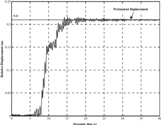
Deterministic permanent horizontal displacement at the slope toe For the slope geometry and the mean values of the soil characteristics described in the previous section, figure 4 presents the toe relative displacement as a function of the dynamic time. This displacement is computed as the difference between the horizontal toe displacement and the horizontal base displacement during the earthquake shaking. The maximum value of this displacement is called the toe permanent horizontal displacement. It is found to be equal to 21 cm as shown in fig. 4.
0 5 10 15 20 25 30 35 40 0 0.05 0.1 0.15 0.2 0.25 Dynamic time (s) R el a tiv e D is p la ce m en t (m) 0.21 Permanent displacement
Fig. 4. Relative displacement at the toe of the slope versus the dynamic time
The contour of shear strain increment that gives an idea about the probable failure surface is presented in figure 5.
Fig. 5. Contour of shear strain increment
System response, limit state surface and probability distribution of the toe permanent displacement
Figure 6 presents the shape of the response surface of the permanent horizontal displacement approximated by the
Fig. 3. North - South component of the “Sour” Event (M=5.1) acceleration registered at Bhannes Station “BHL”.
polynomial chaos expansion using the SRSM method for the case where Cov c20%;Cov G50%.
50 100 150 200 250 10 15 20 25 30 35 400 0.5 1 G (MPa) c (kPa) u ( m )
Fig. 6. Toe permanent displacement as a function of c and G when Cov c20%;Cov G50%.
-5 -4 -3 -2 -1 0 1 2 3 4 5 -4 -3 -2 -1 0 1 2 3 4 u = 30 cm u = 40 cm u = 50 cm u = 70 cm u = 90 cm max max max max max
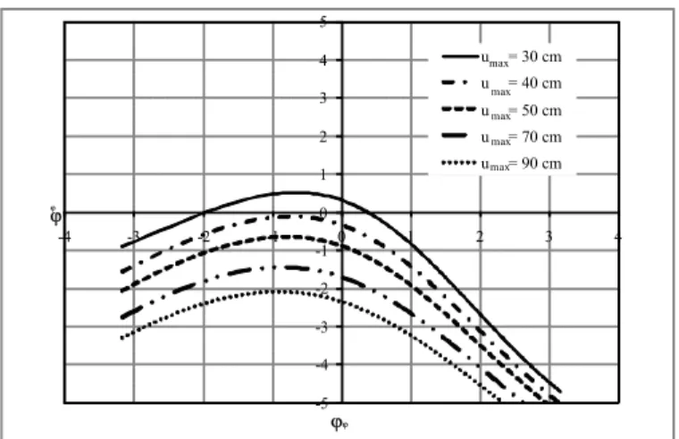
Fig. 7. Limit state surfaces in the standard space of random variables for different values of umax
For different values of an allowable maximal permanent displacement umax, one can plot the limit state surfaces defined by G=u-umax=0 that divides the combinations of
c G,
that would lead to failure (i.e. the exceedance of umax) from the combinations that would not. These limit state surfaces are plotted on figure 7 in the standard space of the random variables for different values of umax varying from 30 cm to 90 cm. One can notice that the limit state surfaces are not linear. Consequently, the classical FORM method that linearly approximates the response surface for the evaluation of the failure probability may lead in this case to inaccurate results. Thus, the determination of the entire probability distribution of the response using the SRSM method is necessary.It was shown earlier in the present paper that the SRSM method allows one to determine the full probability distribution of the system response. The cumulative distribution function of the permanent horizontal displacement is presented in figure 8 for
20%; 50%
Cov c Cov G . The corresponding probability
density function is plotted on figure 9.
0 0.2 0.3 0.4 0.6 0.8 1 1.2 0 0.1 0.2 0.3 0.4 0.5 0.6 0.7 0.8 0.9 1 u (m) CDF Cov c = 20%; Cov G = 50 % 0.7 0.9633
Fig. 8. Cumulative probability function of the permanent horizontal displacement at the toe slope
0 0.2 0.4 0.6 0.7 0.8 1 1.2 0 0.5 1 1.5 2 2.5 u (m) PD F Cov c = 20% ; Cov G = 50% Pf = 3.67 %
Fig. 9. Probability density function of the permanent horizontal displacement at the toe slope
From these functions, the failure probability with respect to the exceedance of an allowable maximum permanent displacement can be easily evaluated. If we consider an allowable maximal permanent displacement umax of 70 cm, the failure probability can be evaluated as follows:
max
1
max
1 0.9633 0.0367 (3.67%)f
P u u u u .
Effect of the coefficients of variation of the random variables on the mean value of the slope permanent displacement
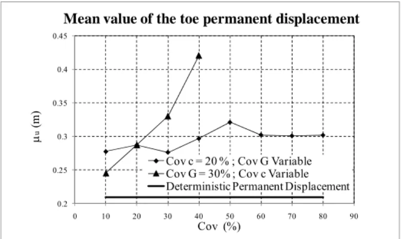
Figure 10 presents the variation of the mean value of the permanent horizontal displacement uat the toe of the slope as a function of the coefficient of variation of the random variables. In this figure, is plotted versus the coefficient of variation of u G and c. For each curve, the coefficient of variation of a
parameter is held to a constant value (20% for the cohesion and 30% for the shear modulus) and the coefficient of variation of the second parameter is varied. The results have shown that is u higher than the deterministic permanent displacement calculated using the mean values of the random variables (i.e.
15 ; 50
c kPa G MPa). It can also be noted that the mean value
of the permanent displacement is highly influenced by the coefficient of variation of the cohesion, the greater the scatter in
c the higher is the permanent displacement. This means that the accurate determination of the distribution of this parameter is very important in obtaining reliable probabilistic results.
0.2 0.25 0.3 0.35 0.4 0.45 0 10 20 30 40 50 60 70 80 90
Mean value of the toe permanent displacement
Cov c = 20 % ; Cov G Variable Cov G = 30% ; Cov c Variable Deterministic Permanent Displacement
u
(m
)
Cov (%)
Fig. 10. Mean of the slope permanent displacement as a function of coefficient of variation of c and G
From the same figure, one can notice that presents a u
maximum value for Cov G50%. In order to understand and
interpret this observation, the mean value of the amplification
A
at the crest of the slope is plotted versus the coefficient of variation of G in figure 11. The amplification in this study refers to the ratio of the maximum output horizontal acceleration at the crest of the slope to the input maximal acceleration at the base of the slope. The amplification is considered here as an output random variable determined by the SRSM. It was noticed that the maximal value of corresponds to the maximal value of A the mean permanent horizontal displacement (i.e. for
50%
Cov G ). One can conclude that for these values of the
soil variability, the amplification of the wave and consequently the mean permanent horizontal displacement of the toe are maximal. 2.35 2.4 2.45 2.5 2.55 2.6 2.65 2.7 0 10 20 30 40 50 60 70 80 90
Mean value of the Amplification
Cov c = 20%; Cov G Variable Deterministic Amplification A m plif ic at io n Cov G
Fig. 11. Mean of the amplification as a function of the coefficient of variation of G
CASE STUDY – BAABDAT SLOPE
A case study of a Lebanese slope situated at Baabdat is presented in this section. This slope is 1.5 km far away from the seismological station “BHL” where the 5.1 magnitude earthquake acceleration record has been registered. The coordinates of the site are: 33.890850oE, 35.660644oN.
The geologic formation of the slope is sandstone, composed by cretaceous sands, mixed with irons, and some intercalation of clay (cf. Figure 12). Since the developed probabilistic models are 2D, the study is done in a 2D cross section. The most critical cross section (AA’) at the middle of the slope (i.e. at the greatest height) was considered. The height of this section is equal to 10 m and the average slope angle is found to be approximately equal to 35o.
Fig. 12. View of a slope cut
Several soil samples were taken in order to perform “Laboratory Direct Shear tests” for the quantification of the variability of the soil shear strength parameters c and . The number of tests carried out at this slope area is 10. The statistical parameters of the soil shear strength were found equal to : c 10 kPa,
25
, COVc 15%, COV 20% . Since it was shown
earlier in this paper that the cohesion and the shear modulus of the soil have the greatest influence on the slope permanent displacement when performing a dynamic analysis, the uncertainties on the friction angle is neglected. It is considered as a deterministic parameter with value equal to its mean value
25
. The range of the Young modulus found in the literature
for a sandstone formation mixed with clay is between 25 and 200MPa. The value of Poisson ratio ranges between 0.25 and 0.33. The corresponding range of the shear modulus varies between 10 and 80 MPa. Consequently, a mean value of 50MPa is used and a high coefficient of variation of 50% is considered. Probability distribution of the permanent horizontal displacement of Baabdat slope
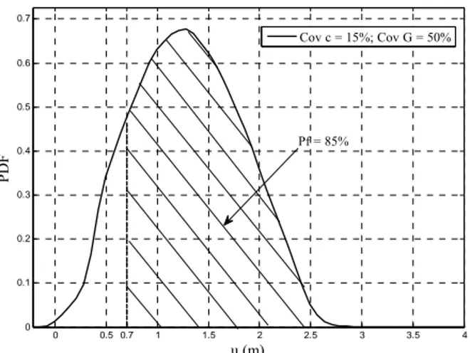
Figure 13 presents the PDF of the permanent displacement of the Baabdat Slope for the same scaled earthquake record presented in figure 3 (amax=2.64cm/s2). By considering an allowable maximal permanent displacement umax of 70 cm, the failure probability is found equal to 85%. This slope is a typical one of the studied region.
It has to be noticed also that the mean value of the permanent displacement is found equal to 1.29 m higher than the deterministic permanent displacement equal to 1.16 m calculated for the mean values of the soil characteristics.
0 0.5 0.7 1 1.5 2 2.5 3 3.5 4 0 0.1 0.2 0.3 0.4 0.5 0.6 0.7 u (m) PD F Cov c = 15%; Cov G = 50% Pf = 85%
Fig. 13. PDF of the permanent displacement when amax=2.64cm/s2
CONCLUSION
This paper examines a dynamic analysis of slope stability using the reliability approach. A numerical simulation is carried through finite difference software. For the acceleration time-history, a record of a local seismic event scaled to 2.68 m/s2 has been used and applied on a local case study slope stability problem. The performance function used in the relability analysis is defined with respect to the permanent displacement at the toe of the slope. It was found that the considered variables cohesion c and shear modulus G of the soil have the most significant effect on displacement.
As for the estimation of the probability distribution of the permanent displacement at the toe, a Stochastic Response Surface Methodology has been adopted. From this approach, it was shown that the mean value of the permanent displacement is very sensitive to the coefficient of variation of the cohesion, the greater the scatter of c the higher is the permanent displacement. Besides, the failure probability is evaluated with respect to the exceedence of an allowable maximal permanent displacement. It was found that the maximal value of the amplification mean A corresponds to the maximal value of the mean permanent displacement (i.e. Cov G50%). One can conclude that for
adopted values of the soil variability, the amplification of the wave and consequently the mean permanent displacement at the toe are maximal.
Finally, the analysis is applied on a case study of a slope in the Baabdat area of the Metn Mountains North of Beirut. This case study representsa typical slope of the studied region. The results showed that when the permanent displacement umax is 70 cm, the failure probability is found equal to 85%. The probabilistic mean value of the permanent displacement found equal to 1.29 m is higher than the deterministic permanent displacement equal to 1.16 m calculated for the mean values of the soil characteristics. REFERENCES
Al-Hamoud, A.S., and Tahtamoni, W.W. "Reliability analysis of three-dimensional dynamic slope stability and earthquake-induced permanent displacement," Soil Dynamics and
Earthquake Engineering, Vol. 19, 91-114, 2000.
Al-Hamoud, A.S., and Tahtamoni, W.W. "Seismic Reliability analysis of earth slopes under short term stability conditions,"
Geotechnical and Geological Engineering, Vol. 20, 201-233,
2002.
Auvinet, G., and Gonzalez, J.L. "Three–dimensional reliability analysis of earth slopes," Computers and Geotechnics, Vol. 26, 247-261, 2000.
Chen, W.F., and Sawada, T. "Earthquake-induced slope failure in nonhomogeneous, anisotropic soils," Soils and Foundations, Vol. 23, N° 2, 125-139, 1983.
Chowdhury, R.N., and Xu, D.W. "Rational polynomial technique in slope-reliability analysis," Journal of Geotechnical
Engineering, ASCE, Vol. 119, N° 12, 1910-1928, 1993.
Christian, J., Ladd, C., and Baecher, G. "Reliability applied to slope stability analysis," J. of Geotech. Engrg., ASCE, Vol. 120, N° 12, 2180-2207, 1994.
Christian, J.T., and Urzua, A. "Probabilistic evaluation of earthquake-induced slope failure," Journal of Geotechnical and
Geoenvironmental Engineering, ASCE, Vol. 124, N° 11,
1140-1143, 1998.
Devroye, L. Non-Uniform Random Variate Generation.
Springer-Verlag, New York, 1986.
El-Ramly, H., Morgenstern, N. R., and Cruden, D. M. "Probabilistic slope stability analysis for practice," Can. Geotech. J., Vol. 39, 665-683, 2002.
Husein Malkawi, A.H., Hassan, W., and Adbulla, F. "Uncertainty and reliability analysis applied to slope stability," Structural Safety, Vol. 22, 161-187, 2000.
Isukapalli S.S. Uncertainty Analysis of
Transport-Transformation Models, Ph.D. Thesis, The State University of
New Jersey, 1999.
Leshchinsky, D., and San, K.-C. "Pseudostatic seismic stability of slopes: Design charts," Journal of Geotechnical Engineering,
ASCE, Vol. 120, N° 9, 1514-1532, 1994.
Loukidis, D., Bandini, P., and Salgado, R. "Stability of seismically loaded slopes using limit analysis," Géotechnique, Vol. 53, N° 5, 463-479, 2003.
Low, B. K., Gilbert, R. B., and Wright, S. G. "Slope reliability analysis using generalized method of slices," Journal of
Geotechnical and Geoenvironmental Engineering, ASCE, Vol.
124, N° 4, 350-362, 1998.
Michalowski, R.L. "Stability charts for uniform slopes," Journal
of Geotechnical and Geoenvironmental Engineering, ASCE,
Vol. 128, N° 4, 351-355, 2002.
Sivakumar Babu, G.L. and Mukesh, M.D. "Effect of soil variability on reliability of soil slopes," Géotechnique, Vol. 54, N°5, 335-337, 2004.
Vanmarcke, E. "Reliability of earth slopes," Journal of the
Geotechnical Engineering, ASCE, Vol. 103, N° GT11,
1247-1265, 1977.
You, L. and Michalowski, R.L. "Displacement charts for slopes subjected to seismic loads," Computers and Geotechnics, Vol. 25, N° 4, 45-55, 1999.
Youssef Abdel Massih, D.S. and Soubra, A.-H. "Reliability-based analysis of strip footings using response surface methodology." International Journal of Geomechanics, ASCE, 8(2), 134-143, 2008.
Youssef Abdel Massih, D.S., Harb, J. and Soubra, A.-H. "Reliability analysis applied on lebanese slopes subjected to seismic loads. " COMPDYN 2009, Computational Methods in
Structural Dynamics and Earthquake Engineering, Rhodes,