HAL Id: hal-01853744
https://hal.archives-ouvertes.fr/hal-01853744
Submitted on 12 Feb 2019
HAL is a multi-disciplinary open access
archive for the deposit and dissemination of
sci-entific research documents, whether they are
pub-lished or not. The documents may come from
teaching and research institutions in France or
abroad, or from public or private research centers.
L’archive ouverte pluridisciplinaire HAL, est
destinée au dépôt et à la diffusion de documents
scientifiques de niveau recherche, publiés ou non,
émanant des établissements d’enseignement et de
recherche français ou étrangers, des laboratoires
publics ou privés.
A generalized Timoshenko beam with embedded
rotation discontinuity
Ibrahim Bitar, Panagiotis Kotronis, Nathan Benkemoun, Stéphane Grange
To cite this version:
Ibrahim Bitar, Panagiotis Kotronis, Nathan Benkemoun, Stéphane Grange. A generalized Timoshenko
beam with embedded rotation discontinuity. Finite Elements in Analysis and Design, Elsevier, 2018,
150, pp.34-50. �10.1016/j.finel.2018.07.002�. �hal-01853744�
A generalized Timoshenko beam with embedded rotation discontinuity
Ibrahim Bitar
a,*, Panagiotis Kotronis
a, Nathan Benkemoun
c, Stéphane Grange
ba École Centrale de Nantes, Université de Nantes, CNRS, Institut de Recherche en Génie Civil et Mécanique (GeM), UMR 6183, 1 rue de la Noë, BP 92101, 44321, Nantes, cedex 3, France b Univ. Lyon, INSA-Lyon, GEOMAS, F-69621, Villeurbanne cedex, France
c IUT Saint-Nazaire, Université de Nantes, CNRS, Institut de Recherche en Génie Civil et Mécanique (GeM), UMR 6183, 58 rue Michel Ange, 44600, Saint-Nazaire, France
A novel generalized Timoshenko beam finite element with higher order shape functions is proposed to simulate structural failure. An embedded rotation discontinuity is adopted at the element level to describe the devel-opment of plastic hinges and crack opening. The material behaviour at the discontinuity is characterized by a discrete linear law linking the bending moment and the rotational jump, which allows capturing the released fracture energy. Outside the discontinuity, the behaviour is reproduced within the framework of elasto-plastic generalized standard materials. The generalized enhanced Timoshenko beam finite element, the variational for-mulation and the specific computational procedures are detailed. Numerical examples of a cantilever beam submitted to a rotation, to a transversal displacement and a two-storey reinforced concrete frame illustrate the capacity of the new beam formulation to regularize the results and to reproduce the structural behaviour up to failure.
1. Introduction
In order to realistically simulate structural behaviour up to failure, one should be able to reproduce strain localization and the opening of cracks. Strain localization occurs prior to rupture for different type of materials: granular materials [1,2], quasi-fragile materials such as con-crete [3,4] and rocks [5,6], materials with an elasto-plastic behaviour with softening [7].
A classical approach to correctly simulate this phenomenon is to add explicitly or implicitly a length scale parameter on the continuum mechanics model by considering a spatial dependency in the constitu-tive equations [8], generally via an integral over space [9] or in a gra-dient form [10–12]. The recent Thick Level-Set (TLS) model [13] is a thermodynamically sound approach with a non constant internal length and a smooth transition from damage to fracture. From a mathematical point of view, the absence of a characteristic length leads to a poorly posed problem; the hyperbolic character of the governing equations is lost [14], causing pathological dependence of the results on the finite element mesh. Numerical analyses showed that fracture is ultimately done without dissipation of energy [15].
* Corresponding author.
E-mail addresses:[email protected](I. Bitar),[email protected](P. Kotronis),[email protected](N. Benkemoun),stephane. [email protected](S. Grange).
Another method, traced back to the work of the Cosserat brothers in the early XXiethcentury [16–20], is to use continua with microstruc-ture. They are kinematically enriched models, whether micromorphic or of the higher order gradient type [21], with additional kinematic description that implicitly introduces a length scale. One of the earliest use of continua with microstructure as a way to regularize the prob-lem of strain localization was introduced by Ref. [22] who adopted a Cosserat type continuum, well suited for granular materials, to cor-rectly model shear banding. This was soon followed with specific kine-matically enriched models [23–25] and theoretical developments for classical and multiphase porous media and case studies for soils and concrete [26–32].
An alternative way is to use rate dependent models by adopting viscoplasticity and a time dependent viscosity parameter [33,34]. In this case, the band width depends not only on the material parameters but also on the load velocity.
A different approach is to treat the localization as a zero-thickness localization zone. A kinematic discontinuity of zero size is intro-duced via a displacement jump (strong discontinuity approach) lead-ing to a slead-ingular deformation field, while the material behaviour is
described via a cohesive law. This method belongs to the family of the Assumed Enhanced Strain Methods [35]. Strain localization occurs in the discontinuity and it is possible to define a dissipative mech-anism which, in turn, allows to capture the same amount of dissi-pated energy regardless the size of the finite element. The approach complies therefore with the two efficiency criteria mentioned by Ref. [36]: ensuring objectivity with respect to the mesh size and tak-ing into account the multi-scale nature of the problem under study. Several methods exist to effectively take into account such discon-tinuities. The main idea is to enhance the classical Finite Element Method (FEM) with additional degrees of freedom that carry the dis-continuities and to make the mesh independent of their presence. A fine mesh or re-meshing is therefore not necessary to simulate crack propagation. The additional degrees of freedom can be carried either by the element nodes, Extended Finite Element Method (X-FEM), or integrated within the element, Embedded Finite Element Method (E-FEM).
The X-FEM introduced in 1999 by Refs. [37–40], is based on the Partition of Unity Method (PUM) [41]. It was initially used with Griffith models and linear fracture mechanics and later for problems with discontinuity surfaces, cohesive models [42,43] and continuum mechanics constitutive laws. The discontinuity is interpolated with specific shape functions added to the classical finite element formu-lation. Cracking can pass through an element by cutting it in half, while the discontinuity variables are incorporated in the mesh at the cracked element nodes. The E-FEM, originally developed by Ref. [44] for modeling strain localization, is based on the Mixed Assumed Strain Approach and more particularly on the method of incompati-ble modes [35]. As in X-FEM, cracks can pass through the elements but the enhanced variables are in this case introduced at the ele-ment and not at the nodal level. This leads to two families of equi-librium equations, one at the global (structural) level and one at the local (element) level. This last one contains the enhanced vari-ables. Static condensation is adopted and therefore the overall res-olution at the structural scale remains the same as in the classical FEM. The E-FEM method can be therefore introduced straightforward to an existing finite element code without any change in its architec-ture.
[45] performed a comparative study on X-FEM and E-FEM. Both methods were implemented in the same finite element code to ensure a reliable comparison. The study shows that both methods provide similar results in terms of quality and quantity for a fairly fine mesh size. For coarse meshes however, E-FEM is generally more precise, while the convergence rate with increasing mesh refinement is slightly higher for X-FEM. From a computational point of view, modeling a single crack with X-FEM leads to a higher computational cost. For multiple cracks, the computational cost of E-FEM remains constant, while it linearly increases with the number of cracks for the X-FEM. The main disadvantage of the E-FEM is that the strain approximations in the two parts of the element separated by a discontinuity are not independent [46].
The objective of this article is to propose a novel generalized Timoshenko beam with higher order interpolation functions capa-ble of reproducing the behaviour of structures up to failure. The Full-Cubic-Quadratic (FCQ) displacement-based Timoshenko beam pro-posed by Ref. [47] is adopted. This formulation uses shape func-tions of order three for the transverse displacements and two for the rotations and has an additional internal node. This results to a Tim-oshenko beam free of shear locking while one beam element pro-vides the exact nodal displacements for whatever loading and suit-able boundary conditions. Comparison of the FCQ beam with vari-ous Timoshenko beams found in the literature (see Refs. [48–50]) is studied in Ref. [51]. In Ref. [51], higher order interpolation func-tions are also adopted for the axial displacements in order to improve the axial force - moment coupling of the initial formulation [47] for non linear problems. The beam section is described through a
stress-resultant constitutive model that takes the form of moment-curvature relation. In order to reproduce failure, a rotation discontinuity is adopted at the element level following the E-FEM method. For sim-plicity reasons and as a first step, only bending failure is thus con-sidered in this paper; shear is elastic and shear failure problems are not addressed. The developments presented are also limited to geo-metrically linear Timoshenko beams. The equilibrium equations are formulated using the initial geometry of the structure and are not updated with the deformation. Validation is provided using classical civil engineering applications (i.e. failure or reinforced concrete struc-tures).
The paper is organized as follows: in the second section, several already published generalized beam finite elements with embedded dis-continuities are presented. In section three, the governing equations of the enhanced FCQ Timoshenko beam with embedded rotation dis-continuity are detailed. The variational formulation is provided in the next section allowing the determination of the enhancement functions. In section five, the generalized constitutive models for the continuum and the cohesive parts are presented and in section six the computa-tional procedures after linearization of the equilibrium equations and the implementation of the generalized laws. The paper ends with sev-eral numerical examples: a cantilever beam submitted to a rotation, to a transversal displacement and a two-storey reinforced concrete frame. These numerical examples illustrate the capacity of the novel beam ele-ment to regularize the results and to reproduce the structural behaviour up to failure.
2. Enhanced generalized beams in the literature
A generalized beam is a beam finite element with stress-resultant constitutive models [52–54]. In this category, we can also integrate the concept of macro-element introduced in geotechnics by Nova and Montrasio [55]. The term enhanced is used for beams with embedded discontinuities.
Armero and Ehrlich [14] were among the first to perform a failure analysis of steel structures using a generalized enhanced Timoshenko beam. The authors adopted elasto-plastic laws, introduced a strong dis-continuity in the rotation field and adopted a cohesive dissipative law (moment-rotation jump) [56]. enhanced the three components of the displacement field (axial, transverse and rotation) and introduced three dissipative mechanisms (three cohesive models). Using an eigenvalue analysis, the authors have shown that high order enhancement func-tions are necessary to avoid shear locking [57]. studied Euler-Bernoulli beams and proposed two enhancements, the first for the axial displace-ment and the second for the rotation field. They showed that the choice of the discontinuity interpolating functions is crucial to obtain accurate results.
[58] combined an enhanced Euler-Bernoulli beam and a shell ele-ment to simulate failure of frame structures. The proposed Euler-Bernoulli beam differs from Ref. [57] as only the rotation component is enhanced [59]. and [60] proposed an enhanced Timoshenko beam for reinforced concrete structures. A scale analysis, using a multi-fiber beam approach, was carried out to identify the parameters of the generalized model [61]. developed an Euler-Bernoulli beam with a bi-linear elasto-plastic behaviour for bending behaviour where only the rotation field was enhanced. Following [59,62] presented a Tim-oshenko beam for reinforced concrete structures considering two rup-ture modes, shear and bending. The transverse and the rotational fields were therefore enhanced. Finally [63], presented a Timoshenko multi-fibre beam element with an axial displacement discontinuity. An elastic-plastic behaviour was considered for steel and damage for concrete to reproduce the behaviour of reinforced concrete structures up to fail-ure.
We present in the following how enhancement (embedded rotation discontinuity) can be taken into account in the novel FCQ Timoshenko beam element formulation [47].
Fig. 1. Beam discontinuities kinematics, enhancement of the rotation field.
3. Enhanced FCQ Timoshenko beam
Consider a beam of length Ł discretized with n FCQ beam elements [47] e = [xi;xj]of length L = xj −xiand external nodes i and j. The
generalized displacement vectorUS(x,t)is approximated by an equation
of the formUS(x,t) = N(x)de(t), wherede(t)is a vector containing the external nodal displacements of the element e andN is the matrix of
the shape functions depending only on x, the beam axis. For sake of simplicity, presentation is made hereafter in 2D.
𝐔S(x,t) = ⎡ ⎢ ⎢ ⎢ ⎣ Ux(x,t) Uy(x,t) Θz(x,t) ⎤ ⎥ ⎥ ⎥ ⎦ = ⎡ ⎢ ⎢ ⎢ ⎣ 𝐍u(x)𝐝 e(t) 𝐍v(x)𝐝 e(t) 𝐍𝜃(x)𝐝 e(t) ⎤ ⎥ ⎥ ⎥ ⎦ (1)
withNu,NvandN𝜃the shape functions of the three components defined by Ref. [47]: ⎡ ⎢ ⎢ ⎢ ⎣ 𝐍u(x) 𝐍v(x) 𝐍𝜃(x) ⎤ ⎥ ⎥ ⎥ ⎦ = ⎡ ⎢ ⎢ ⎢ ⎣ Nu1 0 0 0 0 0 Nu2 0 0 0 N2v 0 N7v 0 N9v 0 Nv5 0 0 0 N3𝜃 0 N8𝜃 0 0 0 N6𝜃 ⎤ ⎥ ⎥ ⎥ ⎦ , (2) where N1u=1−x L Nu 2= x L Nv 2= (1− x L) 2(1+2x L) N7v=2(1−x L) 2(x L) Nv 9= −2( x L) 2(1−x L) Nv 5= ( x L) 2(3−2x L) N𝜃3= (1−x L)(1−3 x L) N𝜃8=1− (1−2x L) 2 N𝜃6= −(x L)(2−3 x L) (3)
deis the nodal displacement vector defined by:
𝐝e= [ Uxi Vyi Θzi ΔVyk1 ΔΘzk ΔVyk2 Uxj Vyj Θzj ]T (4) whereΔV1 yk,ΔΘzkandΔV 2
ykare the degrees of freedom of the internal
node (with no specific physical meaning) [47]. It should be mentioned that only the enhancement of the rotation field is considered hereafter, we are dealing primarily with bending problems, seeFig. 1. This is why first degree polynomial shape functions (Nu
1, N2u) are considered for the axial displacements(3). As already mentioned however, higher order interpolation functions for the axial displacements can be adopted for the FCQ Timoshenko beam in order to improve the axial force
-moment coupling, for more details see Ref. [51]. This does not change the developments presented in this paper.
The enhanced rotation field is written as follows:
Θz(x,t) =𝐍𝜃(x)𝐝e(t) +M(x)Θe(t) (5)
whereΘe(t)represents the discontinuity variable of the rotation field
and M(x)the enhancement function defined as follows:
M(x) =M(x) +Hxd (6)
with xdthe position of the discontinuity within the element and Hxdthe
Heaviside function defined as:
Hxd(x) =
{
1 for x>xd
0 for x<xd (7)
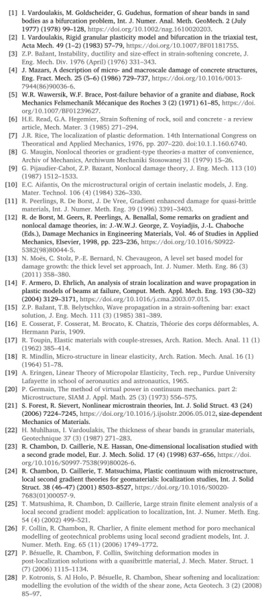
It remains therefore to define the function M(x)and the position of the discontinuity within the element. This requires a good understanding of the beam discontinuity kinematics [57]. Indeed, total failure is reached when there is no more stress transfer through the discontinuity, in our case if the value of the moment at discontinuity is zero [57]. refer to this final deformation state as zero hinge mode.
3.1. Modification of the rotation field shape functions
The enhanced rotation field should reproduce correctly the rotations at the three nodes of the FCQ element (the two external nodes i, j and the internal node k). In the original FCQ Timoshenko beam formulation however, the internal node has not a specific physical meaning,ΔΘzk(t)
does not represent the rotation in the middle (x=L2) of the element [47]. We propose hereafter a slight modification of the interpolation of the rotation field that does not alter the performance of the FCQ beam, it is just used in order to correctly identify the function M(x). The main idea is to provide a physical sense to the internal rotation degree of freedom, the rotation in the middle of the element (x=L2), seeFig. 2.
The rotation in the middle of the elementΘz(L2,t)can be expressed
as a function of the original FCQ shape functions N3𝜃, N6𝜃 and N8𝜃 as follows: Θz(L2,t) = Θzk(t) = ΔΘzk(t) −14 [ Θzi(t) + Θzj(t) ] (8)
with k the index of the internal node positioned in the middle of the FCQ element. The rotation field can be therefore interpolated in the following way: Θz(x,t) =N3𝜃(x)Θzi+N𝜃6(x)Θzj+N𝜃8(x)ΔΘzk =N3𝜃(x)Θzi+N6𝜃(x)Θzj+N𝜃8(x) ( Θzk+1 4[Θzi(t) + Θzj(t)] ) =(N𝜃3(x) +1 4N 𝜃 8(x) ) Θzi+ ( N𝜃6(x) +1 4N 𝜃 8(x) ) Θzj+N𝜃8(x)Θzk =N𝜃 3∗(x)Θzi+N 𝜃 6∗(x)Θzj+N 𝜃 8∗(x)Θzk (9)
Fig. 3. Zero hinge mode (fully opened discontinuity).
Fig. 4. Continuous model.
with the three new interpolation functions:
N3𝜃∗(x) =N𝜃3(x) + 1 4N 𝜃 8(x) =1− 3x L + 2x2 L2 N𝜃 6∗(x) =N 𝜃 6(x) + 1 4N8𝜃(x) = − x L+2 x2 L2 N𝜃 8∗(x) =N 𝜃 8(x) = 4x L − 4x2 L2 (10)
These new shape functions(10) are associated with the three nodal rotation values located at x = 0, x = L and x=L2 and can now be used to correctly identify the function M(x). They verify the classical conditions that must be respected by the shape functions [64]:
N3𝜃∗(0) =1 , N3𝜃∗(L2) =0 , N𝜃3∗(L) =0 N𝜃 6∗(0) =0 , N 𝜃 6∗( L 2) =0 , N𝜃6∗(L) =1 N𝜃 8∗(0) =0 , N 𝜃 8∗( L 2) =1 , N 𝜃 8∗(L) =0 and ∑ 𝛼=3,6,8 N𝛼𝜃∗(x) =1 (11)
The expression of the enhanced rotation field is therefore finally written as: Θz(x,t) =N3𝜃∗(x)Θzi+N6𝜃∗(x)Θzj+N8𝜃∗(x)Θzk+ [ M(x) +Hxd ] Θe(t) (12)
3.2. Identification of the function M(x)
The presence of a discontinuity within a beam element must not affect the compatibility between different elements. In other words, the nodal rotation values at points i and j must not be affected. Following
(12), the following conditions must be met:
For x=0 ∶ Θz(0,t) = Θzi⟹ M(0) =0 For x=L ∶ Θz(L,t) = Θzj⟹ M(L) = −1
(13)
Fig. 6. Path I: Initial and final states.
Fig. 7. Path II: Initial and final states.
The modified FCQ Timoshenko beam has a third internal degree of free-dom carried by a node located in the middle of the element (x=L2), see
Fig. 2. Two cases are studied following the position of the discontinuity xd(xd≤ L2or xd>L2): Θz(L2,t) = Θzk⟹ ⎧ ⎪ ⎨ ⎪ ⎩ si xd≤L 2⟹ M( L 2) = −1 si xd>L 2⟹ M( L 2) =0 (14)
Several functions satisfy the conditions of equations(13) and (14). Nev-ertheless, in order to ensure order compatibility between the enhance-ment functions M(x)and the rotation interpolation functions (N𝜃
3∗(x), N𝜃
6∗(x)and N 𝜃
8∗(x)), M(x)have to be quadratic. If this condition is not met, numerical difficulties may appear [51,65]. The quadratic functions that satisfy the conditions(13)and(14)are:
M(x) = ⎧ ⎪ ⎨ ⎪ ⎩ −(N𝜃 6∗(x) +N 𝜃 8∗(x) ) = −3x L + 2x2 L2 for xd≤L2 −N𝜃 6∗(x) = x L− 2x2 L2 for xd>L2 (15)
3.3. Derivation of the function Gr(x)and discontinuity position Deformation can be obtained by derivation as follows:
𝜺S(x,t) = ⎧ ⎪ ⎪ ⎨ ⎪ ⎪ ⎩ 𝜀(x,t) = 𝜕 𝜕xUx(x,t) 𝛾(x,t) = 𝜕 𝜕xVy(x,t) − Θz(x,t) 𝜅(x,t) = 𝜕 𝜕xΘz(x,t) , (16)
with𝜺S(x,t)the vector of the generalized deformations of the section,
𝜀(x,t),𝛾(x,t)and𝜅(x,t)respectively the axial deformation, shear
defor-Fig. 8. Cantilever beam structure subjected to a rotation.
mation and curvature. Therefore,
𝜺S(x,t) = ⎧ ⎪ ⎨ ⎪ ⎩ 𝜀(x,t) =𝐁𝜀(x)𝐝e(t) 𝛾(x,t) =𝐁𝛾(x)𝐝e(t) 𝜅(x,t) =𝐁𝜅(x)𝐝e(t) +Gr(x)Θe(t) , (17)
with B𝜀(x), B𝛾(x) andB𝜅(x) the derivatives of the shape functions for the three deformation components and Gr(x)the derivative of the
enhancement function M(x)
Gr(x) =Gr(x) +𝛿xd, (18)
with𝛿xdthe Dirac delta function at xd(𝛿xd= ∞for x = xdand𝛿xd=0
otherwise) and Gr(x) = 𝜕M𝜕x(x)calculated as follows:
Gr(x) = ⎧ ⎪ ⎨ ⎪ ⎩ −(B𝜅 6∗(x) +B 𝜅 8∗(x)) = 4x L2 − 3 L for xd≤ L 2 −B𝜅 6∗(x) = − 4x L2 + 1 L for xd> L 2 (19)
Hence, the enhanced curvature is divided into a regular (̃𝜅(x,t)) and a singular (𝜅(x,t)): 𝜅(x,t) =𝐁𝜅(x)𝐝e(t) +Gr(x)Θe(t) ⏟⏞⏞⏞⏞⏞⏞⏞⏞⏞⏞⏞⏞⏞⏞⏟⏞⏞⏞⏞⏞⏞⏞⏞⏞⏞⏞⏞⏞⏞⏟ ̃𝜅(x,t) +𝛿xdΘe(t) ⏟⏟⏟ 𝜅(x,t) (20)
The function M(x)has been previously determined from the three rota-tion nodal values of the FCQ element. The Gr(x)function should be
checked if it is compatible with the zero hinge mode (̃𝜅(x,t) =0), cor-responding to a fully opened discontinuity. The following kinematic relations correspond to the zero hinge mode,Fig. 3:
for xd≤2L (figure 3a) ∶ Θzk= Θzj and Θe= Θzk− Θzi
for xd>L
2 (figure 3b) ∶ Θzk= Θzi and Θe= Θzj− Θzk
(21)
For xd≤L2, using equations(19) and (21)the regular part of the
curva-ture can be expressed as:
̃𝜅(x,t) =𝐁𝜅(x)𝐝e(t) +Gr(x)Θe(t) =B𝜅 3∗(x)Θzi(t) +B 𝜅 6∗(x)Θzj(t) +B 𝜅 8∗(x)Θzk(t) −[B𝜅6∗(x) +B𝜅8∗(x) ] (Θzk(t) − Θzi(t)) (22)
AsΘzk = Θzj(Fig. 3a) finally we get: ̃𝜅(x,t) =(B𝜅3∗(x) +B𝜅6∗(x) +B𝜅8∗(x)
)
⏟⏞⏞⏞⏞⏞⏞⏞⏞⏞⏞⏞⏞⏞⏞⏞⏞⏞⏞⏟⏞⏞⏞⏞⏞⏞⏞⏞⏞⏞⏞⏞⏞⏞⏞⏞⏞⏞⏟
=0 see(11)
Θzi(t) =0, (23)
Equation(23)is always verified as B𝜅 3∗(x) +B
𝜅 6∗(x) +B
𝜅
8∗(x) =0, due to the properties of the shape functions, see(11). If now we repeat the same procedure for the case where xd>2L, this time usingΘzk = Θzi
(Fig. 3b), it can be again found that̃𝜅(x,t) =0. Equation(19)verifies therefore the zero hinge mode state. The discontinuity position can be determined considering the force distribution within the FCQ element. A discontinuity is generated at the point xdwhere the force (bending
moment) reaches its ultimate value. Since the rotation interpolation functions of the FCQ elementN𝜃are quadratic, the curvature is linear and therefore the maximum curvature appears at the ends of the ele-ment at x = 0 or at x = L. For the specific case where the curvature is constant (pure bending), deformation must be constant and there-fore the linear forms of the enhancement function Gr(x)(19) are no
longer appropriate. For this specific case, a constant function is there-fore assumed, Gr(x) = −1L. The discontinuity can appear at any
posi-tion within the element, we decide arbitrarily to fix it in the middle at xd=L2.
The function Gr(x)finally takes the following form depending on the position xdof the discontinuity:
Gr(x) = ⎧ ⎪ ⎪ ⎨ ⎪ ⎪ ⎩ 4x L2 − 3 L for xd=0 −4x L2 + 1 L for xd=L −1 L for xd= L 2 (24) 4. Variational formulation
The Principle of Virtual Work for a beam structure discretized with n FCQ beam elements e of length L is written as:
∑
e
{
Winte −Weext}=0 (25)
with We
intand Wexte the work of the internal and external forces on the
element e respectively.
The work of the internal forces on the element e becomes: Winte = ∫L𝛿𝜺 ∗ S(x,t) T𝐅 S(x,t)dx (26)
with𝛿 the variation symbol, (•)∗ the symbol that indicates that(•)
takes a virtual value,𝜺∗
S(x,t)the vector of the virtual generalized
defor-mations andFS(x,t)the vector of the generalized forces of the section
defined as follows: 𝜺∗ S(x,t) = ⎡ ⎢ ⎢ ⎢ ⎣ 𝜀∗(x,t) 𝛾∗(x,t) 𝜅∗(x,t) ⎤ ⎥ ⎥ ⎥ ⎦ and 𝐅S(x,t) = ⎡ ⎢ ⎢ ⎢ ⎣ Fx(x,t) Fy(x,t) Mz(x,t) ⎤ ⎥ ⎥ ⎥ ⎦ (27)
Fx(x,t), Fy(x,t)and Mz(x,t)are respectively the axial force, the shear
force and the bending moment of the section.
The virtual displacements and virtual deformations are interpolated with the same shape functions as the real ones. An enhanced shape
function Gv(x)is used for the virtual discontinuity variables (see section
4.1for its identification). Gv(x)plays the same role as the Gr(x)
func-tion of secfunc-tion3.3associated with the real discontinuity variables. It should be noted however that the enhanced shape functions Grand Gv
are generally different. The real discontinuity is interpolated following kinematic considerations (section3.2) while the virtual discontinuity is interpolated following static considerations (section4.1). Both inter-polations in the same formulation are first proposed in Refs. [44] and [66].
The virtual enhanced curvature variation𝜅∗(x,t)is (see also
equa-tion(18)):
𝛿𝜅∗(x,t) =𝐁𝜅(x)𝛿𝐝∗
e(t) +Gv(x)𝛿Θ∗e(t)
=𝐁𝜅(x)𝛿𝐝∗e(t) +Gv(x)𝛿Θ∗e(t) +𝛿xd𝛿Θ∗e(t)
(28)
with𝛿Θ∗e(t)the variation of the virtual rotational discontinuity of the element e. Introducing equation(28)in(26)gives:
Winte =𝛿𝐝∗e(t)T𝐅eint,B(t) +𝛿Θ∗e(t)Finte ,G(t) (29) with𝐅eint,B(t)and Feint,G(t)the elementary nodal internal forces defined as: 𝐅e int,B(t) =∫ L𝐁 T(x)𝐅 S(x,t)dx Feint,G(t) =∫ L Gv(x)Mz(x,t)dx (30)
The work of the external forces on the element e becomes: We
ext=𝛿𝐝
∗
e(t)T𝐅eext(t) (31)
with𝐅e
ext(t)the vector of the external forces at the element level.
Introducing equations(29) and (31)in the virtual works principle
(25)makes possible to obtain the balance equation of the structure in the following form:
∑ e { 𝛿𝐝∗ e(t)T𝐅eint,B(t) +𝛿Θ ∗ e(t)Finte ,G(t) −𝛿𝐝 ∗ e(t)T𝐅eext(t) } =0 ⇔ 𝛿𝐝∗ str(t)T ( 𝐅str int,B(t) −𝐅strext(t) ) + n ∑ e 𝛿Θ∗ e(t)Feint,G(t) =0 (32) with𝐝∗
strthe global displacement vector assembling all the virtual nodal
degrees of freedom and n (≤ n) the number of elements where the rota-tion discontinuity is active.
Furthermore, the equilibrium must be respected for all virtual dis-placements𝛿dstr(t) as well as for any elementary virtual jumpΘe(t).
Therefore, we get the following system:
𝐅str int,B(t) −𝐅 str ext(t) =0 ∀e∈1,2, … ,n∶Fe int,G(t) =0 (33)
The first equation in the system (33) represents the overall equilib-rium of the structure, with𝐅str
int,B(t)and𝐅strext(t)the internal and external
forces at the structural level respectively. The size of these vectors is equal to the number of degrees of freedom per node (3 for a 2D prob-lem) multiplied by the total number of nodes. The second equation in
(33)represents the local equilibrium at the level of each rotational dis-continuity inside the element. Considering the decomposition of Gv(x)
in two parts Gv(x)and Gv(x) =𝛿xd, F
e int,G(t)becomes: Finte ,G(t) = ∫L Gv(x)Mz(x,t)dx=∫ L (Gv(x) +Gv(x))Mz(x,t)dx = ∫L Gv(x)Mz(x,t)dx+∫ L Gv(x)Mz(x,t)dx=0
and as a result
∫L
Gv(x)Mz(x,t)dx= −∫ L𝛿xd
Mz(x,t)dx= −Mz(xd,t) = −Cm(t) (34)
where Cm(t)is the cohesive bending moment at xd.
4.1. Identification of the function Gv
As already mentioned, the enhanced shape function Gv(x)is used for
the virtual discontinuity variables and plays the same role as the func-tion Gr(x)associated with the real discontinuity variables. The function
Gv(x)is often considered equal to Gr(x). This however is not possible
for the enhanced FCQ Timoshenko beam element formulation as shown hereafter.
At the discontinuity position xd, the equality (34) between the
cohesive bending moment Cm(t)and the generalized bending moment
Mz(xd,t)should be verified. Since the moment takes a linear form (see
section3.3), it can be expressed as:
Mz(x,t) =𝛼x+𝛽 (35)
with𝛼and𝛽 constants. For the case where xd = 0, we have Gr(x) =
4x
L2 −
3
L (24). Considering Gv(x) =Gr(x) and introducing the latter in
(34)we get: Cm(t) = −∫ L Gv(x) ⏟⏟⏟ =Gr(x) Mz(x,t)dx = − ∫L (4x L2 − 3 L ) (𝛼x+𝛽)dx=5L 3𝛼 −2𝛽≠𝛽 =Mz(0,t) (36) In other words and for xd = 0, the equilibrium condition(34) is
not verified if Gv(x)is considered equal to Gr(x). The way to correctly
identify Gv(x)is to consider the local equilibrium condition(34) and the Patch test.
4.1.1. Local equilibrium condition Let’s assume the following linear form:
Gv(x) =cx+d (37)
with c and d constants to be determined by verifying the local equilib-rium condition Cm(t) = Mz(xd,t). We get:
Cm(t) = − ∫L Gv(x)Mz(x,t)dx= − ∫L (cx+d) (𝛼x+𝛽)dx =𝛼 ( −cL3 3 −d L2 2 ) +𝛽 ( −cL2 2 −dL ) (38) and Mz(xd,t) =𝛼xd+𝛽 (39)
The equality of the equations(38) and (39)gives the following results:
𝛼xd+𝛽 = 𝛼 ( −cL3 3 −d L2 2 ) +𝛽 ( −cL2 2 −dL ) (40)
The identification of the two sides of the equation(40)provides:
c= 6 L2 − 12 L3xd d= −4 L+ 6 L2xd (41)
and the enhancement function Gv(x)associated with a discontinuity at xdbecomes: Gv(x) =(6 L2 − 12 L3xd ) x−4 L+ 6 L2xd (42)
Finally, the enhancement function Gv(x)of the virtual rotational
dis-continuity takes the following forms depending on the position xdof
the discontinuity inside the FCQ Timoshenko beam element:
Gv(x) = ⎧ ⎪ ⎪ ⎨ ⎪ ⎪ ⎩ 6x L2 − 4 L for xd=0 −6x L2 + 2 L for xd=L −1 L for xd= L 2 (43) 4.1.2. Patch test
An additional verification is required to finally validate the Gv(x)
function. The enhancement with integrated discontinuities is similar to the incompatible modes method and therefore the enhancement func-tion should verify the Patch test [67]. This test, initially proposed by Ref. [68], reflects a convergence condition when refining the mesh. A large number of elements results in small dimension elements and con-sequently elementary strains and stresses should converge to constant values. The Patch test guarantees the ability to represent a constant state of stress per element [69].
The application of the Patch test requires that the additional virtual work associated with the enhancement is zero if the bending moment is constant along the element:
𝛿Θe(t)Finte ,G(t) =0 𝛿Θe(t)∫
L
Gv(x)Mz(x,t)dx=0
Since Mzis constant per element⇒⏟⏞⏞⏞⏞⏞⏞⏟⏞⏞⏞⏞⏞⏞⏟𝛿Θe(t)Mz(x,t)
≠0 ∫L Gv(x)dx=0 ⇒ ∫L Gv(x)dx=0 (44)
The introduction of the two components (regular and singular) of Gv(x)
gives: ∫L ( Gv(x) +Gv(x) ) dx= ∫L ( Gv(x) +𝛿xd)dx=0 (45) Therefore and in order to verify the Patch test the condition is:
∫L
Gv(x)dx= −1 (46)
Using the expressions of Gv(x)provided in(43)it can be verified that
the Patch test(46)is satisfied.
5. Generalized models
A simple stress resultant model is considered hereafter, where the generalized forces (axial force, shear force and bending moment) are expressed respectively as a function of the generalized deformations (axial deformation, shear deformation and curvature). The axial and transverse behaviour are supposed elastic:
Fx(x,t) =EA𝜀(x,t) Fy(x,t) =kGA𝛾(x,t) (47)
where E the Young modulus, G the shear modulus, A the section area and k the shear correction factor [70].
For the bending behaviour, a continuous/cohesive coupled model formulated within the framework of the generalized standard materials [71] is introduced. The variables associated with the continuous model are surmounted by a bar, while the variables of the cohesive model by a double bar. Variables with no bars are associated with the coupling of the two models.
Fig. 10. Cantilever beam structure subjected to a rotation - Global response (bending moment - imposed rotation), FCQ elements with the same material characteristics.
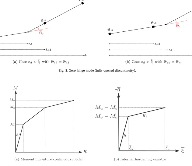
5.1. Continuous model
A generalized elasto-plastic model with an isotropic bi-linear hard-ening (Fig. 4) is adopted. This simple model is chosen as it is sufficient for several civil engineering applications (see section7). Actually, it allows reproducing the three main phases of the reinforced concrete behaviour (elastic, concrete damage, steel plastification). The develop-ment of the generalized law follows the classical framework of plastic-ity. More specifically:
∙The generalized continuous curvature𝜅(x,t)is partitioned into an elastic𝜅e(x,t)and a plastic𝜅p(x,t)component [72]:
𝜅(x,t) =𝜅e(x,t) +𝜅p(x,t) (48) ∙The moment curvature relation is written as
M(x,t) =EI𝜅e(x,t) =EI(𝜅(x,t) −𝜅p(x,t)) (49) with I the moment of inertia.
∙The yield condition𝜙is expressed as:
𝜙(M,q) =|M|− (Mc−q)≤ 0 (50)
where M the current bending moment, Mcthe elastic limit (flow stress),
Mythe value where the second slope change occurs and Muthe failure
(ultimate) bending moment of the moment curvature continuous model
Fig. 11. Cantilever beam structure subjected to a rotation - Global response (bending moment - imposed rotation), presence of a default in the first FCQ element (Me=1
u 272 kN m instead of 274 kN m).
Fig. 12. Cantilever beam structure subjected to a rotation 1 FCQ element -Material behaviour outside the discontinuity.
(Fig. 4a). q is the stress-like internal hardening variable defined as:
q= ⎧ ⎪ ⎨ ⎪ ⎩ −H1𝜉 for 𝜉≤𝜉y −(My−Mc)(1− H2 H1) −H2𝜉 for 𝜉 > 𝜉y (51)
with H1 and H2 the two plastic moduli,𝜉≥ 0 the strain-like internal hardening variable and𝜉y=
My−Mc
H1 (Fig. 4b).
∙ An associated plasticity is considered, the flow rule and the isotropic hardening law become (the principle of maximum plastic dissipa-tion is as usual adopted to determine the evoludissipa-tion of the internal variables):
̇𝜅p= ̇𝛾sign(M) ̇𝜉 = ̇𝛾 (52)
where𝛾is the slip rate and sign(•)defines the sign of the variable(•).
∙ The Kuhn-Tucker complementarity conditions are [72]:
̇𝛾≥ 0 𝜙≤ 0 ̇𝛾𝜙 =0 (53)
∙ The consistency condition is [72]:
̇𝛾 ̇𝜙 =0 (54)
Fig. 13. Cantilever beam structure subjected to a rotation 1 FCQ element -Material behaviour at the discontinuity.
Fig. 14. Cantilever beam structure subjected to a transversal displacement.
For a plastic step, the slip rate ̇𝛾 must be positive (not zero), so the rate of the yield surface ̇𝜙must be zero. This allows determining ̇𝛾as follows: ̇𝛾 = ⎧ ⎪ ⎪ ⎨ ⎪ ⎪ ⎩ Eİ𝜅 EI+H1 if 𝜉≤𝜉y Eİ𝜅 EI+H2 otherwise (55)
∙Substitution of the last equation(55)in equation(49)finally gives:
̇ M= ⎧ ⎪ ⎪ ⎨ ⎪ ⎪ ⎩ Eİ𝜅 if ̇𝛾 =0 EI ( 1− EI EI+H1 ) ̇𝜅 if 𝜉≤𝜉y EI ( 1− EI EI+H2 ) ̇𝜅 otherwise (56) 5.2. Cohesive model
The works of [73] and [74] are the first dealing with the devel-opment of cohesive models, models that link a stress to a displace-ment jump. They constitute an intermediate approach between con-tinuum and fracture mechanics and are considered as an extension of the Griffith’s theory [75] since they allow modeling crack initiation and evolution (see for example [43,76]). A significant improvement of this approach was proposed in Ref. [77] by introducing the concept of frac-ture energy and the critical stress beyond which the crack is supposed to propagate. The transition from the continuous to the cohesive model occurs when a criterion, often based on the stress state, is verified. As soon as the stress value (in our case the bending moment) at a given location exceeds the failure moment Mu, the discontinuity and its
cohe-sive behaviour law are activated. Several cohecohe-sive laws exist in the lit-erature according to the type of the material and the loading envisaged, [43,76]. Since only monotonic loadings are considered in this paper, a linear cohesive law is adopted hereafter for simplicity.
In the following, the adopted cohesive model links the cohesive bending moment Cmto a rotation jumpΘewith a linear law (Fig. 5). The cohesive relation is written as:
Cm=SΘe+Mu (57)
with S (negative value) the softening modulus. Muand S are chosen from experimental studies [78,79] or multiscale identification calcula-tions [59,60].
The discontinuity represents a cohesive zone of zero thickness positionned at xd (where the failure moment Mu is reached). As for the case of the continuous model, discontinuity activation is provided with a failure condition that takes the following form:
𝜙(Cm, Θe) =|Cm|− (Mu+SΘe)≤ 0 (58)
After the activation of a discontinuity within the beam finite element, it is assumed that outside the material unloads elastically (the dissi-pation phenomena are supposed negligible outside the discontinuity, they only develop inside the cohesive zone [80]). Among the inter-nal variables that verify the failure criterion, those that maximize the cohesive dissipation are selected. As for the continuous elasto-plastic formulation, a minimization problem of free energy under con-straint is solved and the discontinuity evolution equation becomes:
̇
Θe= ̇𝛾sign(Cm) (59)
The Kuhn-Tucker complementarity conditions are:
̇𝛾≥ 0, 𝜙≤ 0, ̇𝛾 𝜙 =0 (60) and the consistency condition:
̇𝛾 ̇𝜙 =0 (61)
When a discontinuity is active, the multiplier ̇𝛾 is strictly pos-itive. Thus, in order to verify the consistency condition 𝜙 =̇ 0. Using the equations (58) and (59) this finally results to:
̇ 𝜙 =|Ċm|−S ̇ Θe ⇒ 0=|Ċm|−S ̇ Θe ⇒ 0=|Ċm|−Ṡ𝛾sign(Cm) ⎫ ⎪ ⎪ ⎪ ⎬ ⎪ ⎪ ⎪ ⎭ ⟹̇𝛾 = 1S|Ċm|=1SĊmsign(Cm) (62) 6. Numerical implementation
After the presentation of the variational formulation, the enhanced generalized Timoshenko beam formulation and the continuous and cohesive laws, the computational implementation is detailed hereafter.
6.1. Linearization of equilibrium equations
The two equilibrium equation(33), repeated hereafter as equation
(63), must be checked at each calculation step.
𝐅str int,B(t) −𝐅 str ext(t) =0 ∀e∈1,2, … ,n∶Feint,G(t) =0 (63)
Equation(63)are generally non-linear. To solve them with the Newton-Raphson method they must be first linearized to obtain a system of linear coupled equations in a matrix form.
Suppose that all variables are known at t, we need to calculate them at t+1 (time step t + 1). The residualR of the first (global) equation
of(63)is defined as: 𝐑(𝐝str, Θ1, Θ2, … , Θn) =𝐅strint,B(t) −𝐅 str ext(t) = n A e=1 { 𝐅e int,B−𝐅 e ext } (64) with ⎧ ⎪ ⎪ ⎨ ⎪ ⎪ ⎩ 𝜕𝐑 𝜕𝐝str = n A e=1 (𝜕𝐅e int,B 𝜕𝐝e ) 𝜕𝐑 𝜕Θe =𝜕𝐅 e int,B 𝜕Θe ∀e∈n (65) Table 1
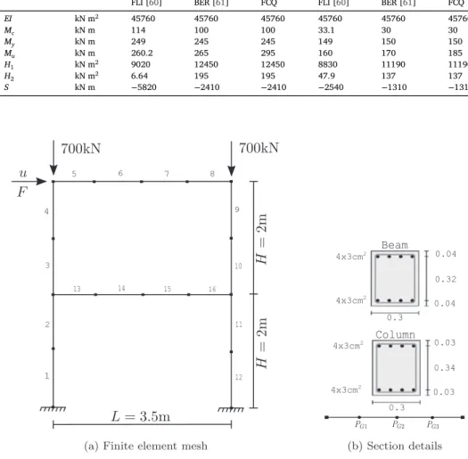
Cantilever beam structure subjected to a transversal displacement - Properties of the generalized model.
EI (kN m) Mc(kN m) My(kN m) Mu(kN m) H1(kN m−2) H2(kN m−2) S (kN m)
Fig. 15. Cantilever beam structure subjected to a transversal displacement - Global Response and mesh sensitivity.
de andΘe are respectively the vector of the continuous elementary nodal displacements and the elementary rotational discontinuity, As before, n is the total number of elements, n≤ n the number of elements where a discontinuity appears and L the length of the element e. Lin-earization of equation(64)is done using an iterative procedure (the k index is used for the iterations) to achieve structural equilibrium. For the time step t+1 we have:
𝐑|(k+1) t+1 =𝐑| (k) t+1+ 𝜕𝐑𝜕𝐝 str| (k) t+1Δ𝐝str|(t+k+11)+ n ∑ e=1 ⎧ ⎪ ⎨ ⎪ ⎩ 𝜕𝐑 𝜕Θe |(k) t+1ΔΘe|(tk++11) ⎫ ⎪ ⎬ ⎪ ⎭ =0 =𝐑|(k) t+1+ n A e=1 ⎧ ⎪ ⎪ ⎨ ⎪ ⎪ ⎩ 𝜕𝐅e int,B 𝜕𝐝e | (k) t+1 ⏟⏞⏞⏞⏟⏞⏞⏞⏟ 𝐊BB · Δ𝐝e|(k+1) t+1 ⎫ ⎪ ⎪ ⎬ ⎪ ⎪ ⎭ + n ∑ e=1 ⎧ ⎪ ⎪ ⎪ ⎨ ⎪ ⎪ ⎪ ⎩ 𝜕𝐅e int,B 𝜕Θe |(k) t+1 ⏟⏞⏞⏞⏟⏞⏞⏞⏟ 𝐊BG · ΔΘe|(tk++11) ⎫ ⎪ ⎪ ⎪ ⎬ ⎪ ⎪ ⎪ ⎭ =0 (66)
Following the definition of𝐅e
int,B(see equation(30)), one can write:
𝐊BB= 𝜕𝐅e int,B 𝜕𝐝e = 𝜕 𝜕𝐝e ( ∫L𝐁( x)T𝐅 S(x,t)dx ) = ∫L𝐁( x)T𝜕𝐅S 𝜕𝐝e (x,t)dx =∫ L𝐁( x)T𝜕𝐅S 𝜕̃𝜺S (x,t)𝜕̃𝜺S 𝜕𝐝e (x)dx (67) = ∫L𝐁( x)T𝜕𝐅S 𝜕̃𝜺S (x,t)𝐁(x)dx and 𝐊BG= 𝜕𝐅e int,B 𝜕Θe = 𝜕 𝜕Θe ( ∫L𝐁( x)T𝐅S(x,t)dx ) = ∫L𝐁 𝜅(x)T𝜕Mz 𝜕Θe (x,t)dx = ∫L𝐁 𝜅(x)T𝜕Mz 𝜕̃𝜅 (x,t) 𝜕̃𝜕Θ𝜅 e (x)dx (68) = ∫L𝐁 𝜅(x)T𝜕Mz 𝜕̃𝜅 (x,t)Gr(x)dx
Therefore, equation(66)can be reformulated in a matrix form (see also equation(64)): n A e=1 ⎧ ⎪ ⎨ ⎪ ⎩ [ 𝐊BB 𝐊BG ](k) t+1 ⎡ ⎢ ⎢ ⎣ Δ𝐝e ΔΘe ⎤ ⎥ ⎥ ⎦ (k+1) t+1 ⎫ ⎪ ⎬ ⎪ ⎭ = −𝐑|(t+k)1= − n A e=1 { (𝐅eint,B−𝐅exte )|(tk+)1} (69) In a similar way, the second (local) equation of(63)is linearized using an iterative procedure (the l index is adopted for the local iterations). For the time step t+1 and considering a fixed displacement increment
Δdeat the element (local) level for the iteration k we have:
Fe int,G|(l+1)=Finte ,G|(l)+ 𝜕Fe int,G 𝜕𝐝e | (l)Δ𝐝 e|(tk+)1+ 𝜕Fe int,G 𝜕Θe |(l)ΔΘ e|(l+1)=0 =Fe int,G|(l)+𝐊GB|(l)Δ𝐝e|(tk+)1+KGG|(l)ΔΘe|(l+1)=0 (70)
According to Feint,Gin equation(34), one can thus write:
𝐊GB= 𝜕Fe int,G 𝜕𝐝e = 𝜕 𝜕𝐝e ( ∫L Gv(x)TMz(x,t)dx ) = ∫L Gv(x)T𝜕𝜕𝐝Mz e (x,t)dx = ∫L Gv(x)T𝜕 Mz 𝜕̃𝜅(x,t) 𝜕̃𝜕𝐝𝜅e (x)dx (71) =∫ L Gv(x)T𝜕 Mz 𝜕̃𝜅(x,t)𝐁𝜅(x)dx and KGG= 𝜕Fe int,G 𝜕Θe = 𝜕 𝜕Θe ( ∫L Gv(x)TMz(x,t)dx ) +𝜕Cm(t) 𝜕Θe = ∫L Gv(x)T𝜕 Mz 𝜕Θe (x,t)dx+𝜕Cm(t) 𝜕Θe =∫ L Gv(x)T𝜕 Mz 𝜕̃𝜅 (x,t) 𝜕̃𝜕Θ𝜅 e (x)dx+𝜕Cm(t) 𝜕Θe = ∫L Gv(x)T𝜕Mz 𝜕̃𝜅 (x,t)Gr(x)dx+𝜕 Cm(t) 𝜕Θe (72) with𝜕Cm(t) 𝜕Θe
=S the softening modulus of the cohesive model (see equa-tion(57)). Finally, assembling the local equation(70) of all the ele-ments yields:
Fig. 16. Two-storey reinforced concrete frame - Geometry and reinforced concrete section details [86]. n A e=1 ⎧ ⎪ ⎨ ⎪ ⎩ [ 𝐊GB KGG ](k) t+1 ⎡ ⎢ ⎢ ⎣ Δ𝐝(ek) ΔΘ(el+1) ⎤ ⎥ ⎥ ⎦t+1 = −Fe int,G| (l) t+1 ⎫ ⎪ ⎬ ⎪ ⎭ (73)
Finally, equations(69) and (73)can be written in a single system as:
n A e=1 ⎧ ⎪ ⎨ ⎪ ⎩ [ 𝐊BB 𝐊BG 𝐊GB KGG ](l) t+1 ⎡ ⎢ ⎢ ⎣ Δ𝐝e ΔΘe ⎤ ⎥ ⎥ ⎦ (k+1) t+1 = ⎡ ⎢ ⎢ ⎣ −(𝐅eint,B−𝐅eext) −Fe int,G ⎤ ⎥ ⎥ ⎦ (k) t+1 ⎫ ⎪ ⎬ ⎪ ⎭ (74)
The local variableΔΘecan be solved by static condensation at the ele-ment level [81]. The main advantage of the static condensation method is that the enhanced degrees of freedom are solved at the element (local) level and therefore the total number of degrees of freedom at the struc-tural (global) level remains unchanged. After convergence of the inter-nal discontinuities variables, we should have Finte ,G|t+1=0. The system then becomes: n A e=1 ⎧ ⎪ ⎨ ⎪ ⎩ [ 𝐊BB 𝐊BG 𝐊GB KGG ](l) t+1 ⎡ ⎢ ⎢ ⎣ Δ𝐝e ΔΘe ⎤ ⎥ ⎥ ⎦ (k+1) t+1 = ⎡ ⎢ ⎢ ⎣ −(𝐅e int,B−𝐅eext) 0 ⎤ ⎥ ⎥ ⎦ (k) t+1 ⎫ ⎪ ⎬ ⎪ ⎭ (75)
The second equation of the system gives: [ 𝐊GB|(l)Δ𝐝e+KGG|(l)ΔΘe ](k+1) t+1 =0 (76) and therefore ΔΘe|(tk++11)= −K −1 GG| (l)𝐊 GB|(l)Δ𝐝e|t(k++11) (77) Table 2
Two-storey reinforced concrete frame - Generalized cross-sectional model parameters.
Variable Description
Mc Bending moment corresponding to the first crack in concrete fibers
My Bending moment beyond which steel fibers enter into plasticity
Mu Failure moment
EI Bending stiffness
H1 First hardening modulus (continuum model)
H2 Second hardening modulus (continuum model)
S Softening modulus (cohesive generalized model)
The use of the latter expression in the first equation of the system(75)
yields: 𝐊BB|(l)Δ𝐝e|(t+k+11)+𝐊BG|(l)(−K−GG1|(l)𝐊GB|(l)Δ𝐝e)|(tk++11) = −(𝐅eint,B−𝐅eext)|(tk++11) (78) and consequently ( 𝐊BB|(l)−𝐊BG|(l)KGG−1| (l)𝐊 GB|(l) ) ⏟⏞⏞⏞⏞⏞⏞⏞⏞⏞⏞⏞⏞⏞⏞⏞⏞⏞⏞⏞⏞⏞⏞⏞⏟⏞⏞⏞⏞⏞⏞⏞⏞⏞⏞⏞⏞⏞⏞⏞⏞⏞⏞⏞⏞⏞⏞⏞⏟ 𝐊e cond|( l) Δ𝐝e|t+1 = −(𝐅eint,B−𝐅eext)|(tk++11) (79) with𝐊e
condthe condensed stiffness matrix.
After the assembly of the element internal forces and stiffness matri-ces, the internal force vector of the structure𝐅str
int,B is introduced in
the equation of the residual𝐑(tk++11) (64). If𝐑(tk++11) tends to zero, the next time step is triggered. Otherwise, another iteration (k + 2) is per-formed within the same time step t+ 1. A new displacement increment is calculated as follows: 𝛿Δ𝐝(k+2) e,t+1 = ( 𝐑(k+1) t+1 )−1 𝐊(k+1) t+1 (80)
with𝐊(tk++11) the global stiffness matrix after the assembly of the ele-mentary stiffness matrices. The new displacement increment of the step t+1 is: Δ𝐝(ek,t++21)= k∑+2 i=1 𝛿Δ𝐝(i) e,t+1 (81)
The calculation procedure is repeated until both equilibrium equations (local and global) are verified. Once the equilibrium is reached, the internal variables and the structure displacement vector are updated as follows: 𝐝(kconv) e,t+1 =𝐝 (k) e,t+1+ Δ𝐝 (kconv) e,t+1 (82)
Table 3
Two-storey reinforced concrete frame - Generalized cross-sectional model parameters of columns and beams for the FLI [60], the Euler-Bernoulli [61] and the FCQ elements.
Parameter Unit Columns Beams
FLI [60] BER [61] FCQ FLI [60] BER [61] FCQ
EI kN m2 45760 45760 45760 45760 45760 45760 Mc kN m 114 100 100 33.1 30 30 My kN m 249 245 245 149 150 150 Mu kN m 260.2 265 295 160 170 185 H1 kN m2 9020 12450 12450 8830 11190 11190 H2 kN m2 6.64 195 195 47.9 137 137 S kN m −5820 −2410 −2410 −2540 −1310 −1310
Fig. 17. Two-storey reinforced concrete frame - Discretization, loading and section reinforcement details.
6.2. Computation of the generalized constitutive model variables
The evolution of the variables associated with the continuous (𝜅p, 𝜉)
and the cohesive model (Θe) is calculated at each gauss point and for
each iteration k. Since only monotonic loading is considered in this
Fig. 18. Two-storey reinforced concrete frame - Numerical and experimental global results (force - horizontal displacement), FCQ, FLI and BER formulations.
study, the two groups of variables cannot evolve simultaneously. Either the continuous model is active and only its internal variables evolve, either the cohesive model is active and outside the discontinuity the material undergoes an elastic unloading (see also section5.2). The res-olution procedure can therefore take two different paths (Path I and
Fig. 19. Two-storey reinforced concrete frame - Numerical and experimental global results (force - horizontal displacement), FCQ, FLI and BER formulations (zoom between 0 and 0.16 m of imposed axial displacement).
Fig. 20. Two-storey reinforced concrete frame - Progressive development of discontinuities, FCQ formulation.
Fig. 21. Two-storey reinforced concrete frame - Progressive development of discontinuities on the global response curve, FCQ formulation.
Path II) depending on the discontinuity state.
Numerical implementation follows the Return-Mapping algorithms [82] and are based on the work of [58] and [83]. An implicit backward Euler integration scheme is adopted that takes the following general form (v = 1): xn+1=xn+ Δx ⏞⏞⏞ Δtẋn+v xn+v=vxn+1+ (1−v)xn;v∈ [0,1] (83)
6.2.1. Plastic model variables
The Path I (seeFig. 6) initial(t)and final(t + 1)states are: Calculation is initiated assuming an elastic predictor:
𝜅p,trial t+1 =𝜅 p t 𝜉trial t+1=𝜉t (84)
The generalized moment and the hardening variable (stress-like) are cal-culated as: Mtrial z,t+1=EI [ 𝜅(d(ek,t−+11), Θie,(,tk+−11) ) −𝜅pt+,trial1 ] (85) qtrial t+1= ⎧ ⎪ ⎨ ⎪ ⎩ −H1𝜉trial t+1 if 𝜉≤𝜉y −(My−Mc)(1− H2 H1 ) −H2𝜉trial otherwise (86)
This makes possible to calculate𝜙as:
𝜙trial
t+1=|Mztrial,t+1|− (Mc−qtrialt+1)≤ 0 (87) If the last equation is verified then the step is elastic and the plastic and hardening variables do not change:
𝜅p t+1=𝜅 p,trial t+1 𝜉t+1=𝜉trialt+1 Mz,t+1=Mtrialz,t+1 qt+1=qtrialt+1 (88)
If the stress state exceeds the elastic limit (𝜙trial>0), then the step is
plastic and the variables are updated:
𝜅p t+1=𝜅 p n+𝛾t+1sign(Mtrialz,t+1) 𝜉t+1=𝜉n+𝛾t+1 Mz,t+1=Mtrialz,t+1−𝛾t+1EI sign(Mz,t+1) (89)
with𝛾t+1the plastic multiplier calculated for𝜙t+1=0. The following property is used to resolve𝜙t+1=0:
sign(Mz,t+1) =sign(Mztrial,t+1) (90) This can be seen from equation(89)as follows:
|Mz,t+1| sign(Mz,t+1) =|Mztrial,t+1| sign(M
trial
z,t+1) −𝛾t+1EI sign(Mz,t+1)
(|Mz,t+1|+𝛾t+1EI)sign(Mz,t+1) =|Mztrial,t+1| sign(M
trial z,t+1)
(91)
By definition𝛾t+1≥ 0 and therefore equation(91)provides:
sign(Mz,t+1) =sign(Mztrial,t+1) (92) along with
|Mz,t+1|=|Mztrial,t+1|−𝛾t+1EI (93) The updated stress-like hardening variable is:
qt+1= ⎧ ⎪ ⎪ ⎨ ⎪ ⎪ ⎩ qtrialt+1−H1𝛾t+1 if 𝜉 < 𝜉t+1< 𝜉y qtrial t+1− (H2−H1)(𝜉t−𝜉y) −H2𝛾t+1 if 𝜉t≤𝜉y, 𝜉t+1> 𝜉y qtrialt+1−H2𝛾t+1 if 𝜉t+1> 𝜉t> 𝜉y (94) Introducing equations(94) and (93)in the yield surface𝜙t+1provides the updated plastic multiplier𝛾t+1as:
𝛾t+1= ⎧ ⎪ ⎪ ⎪ ⎪ ⎨ ⎪ ⎪ ⎪ ⎪ ⎩ 𝜙trial t+1 EI+H1 if 𝜉 < 𝜉t+1< 𝜉y 𝜙trial t+1− (H2−H1)(𝜉t−𝜉y) EI+H2 if 𝜉t≤𝜉y, 𝜉t+1> 𝜉y 𝜙trial t+1 EI+H2 if 𝜉t+1> 𝜉t> 𝜉y (95)
Finally, the discontinuity activation criterion within the element must be verified. The fracture surface𝜙(Ct+1,Ut+1)is first calculated and the cohesive force is found from equation(34):
Cm,t+1= −∫ L 0 Gv(x)Mz,t+1(x)dx= −L2 npg ∑ pg Gv(xpg)Mz,t+1(xpg)w(xpg) (96) with npg the number of integration points along the beam ele-ment and w(xpg) the associated integration weight of point xpg. If 𝜙(Cm,t+1, Θe,t+1)≤ 0, computation continues without activating the dis-continuity. If𝜙(Cm,t+1, Θe,t+1)>0 the discontinuity is activated and all the updated values of the internal variables associated with the contin-uous model in this iteration are not considered. Calculation is re-started following the path II explained in the next paragraph.
6.2.2. Cohesive model variables
Path II (seeFig. 7) is followed when a discontinuity is active. In this case, only the variables associated with the cohesive model evolve. Outside the discontinuity the material undergoes elastic unloading and therefore the variables of the plastic model retain the values of the previous time step. The Path II initial(t)and final(t+ 1)states are:
The elastic predictor is written as:
Θtrial
e,t+1= Θe,t (97)
The trial cohesive force Ctrial
t+1=Ft+1(xd)at the discontinuity level xdis
determined using equation(34)as follows:
Cmtrial,t+1= − ∫L Gv(x)Mtrialz,t+1(x)dx= − L 2 npg ∑ pg Gv(xpg)Mztrial,t+1(xpg)w(xpg) (98) with Mztrial,t+1(xpg) =EI(xpg) ( B(xpg)d(ek,t−+11)+G(xpg)Θtriale,t+1−𝜅 p t ) (99)
The failure sufrace𝜙trialt+1 must be evaluated to check whether the dis-continuity is activated or not:
𝜙trial
t+1=|Cmtrial,t+1|− (Mu+SΘtriale,t+1)≤ 0, (100) If the previous equation is verified then discontinuity is not active and the corresponding variables retain the predicted values:
Θe,t+1= Θtriale,t+1 Cm,t+1=Ctrialm,t+1
(101)
If𝜙trial
t+1>0 then the discontinuity is active. The new admissible values of the variables associated with the cohesive model are calculated using the implicit backward Euler integration scheme:
Θe,t+1= Θe,t+ Δ𝛾sign(Ctrial
m,t+1) (102)
The updated cohesive force at the step t + 1 is written: Cm,t+1= − ∫L Gv(x)Mz,t+1(x)dx = −∫ L Gv(x)EI ( Bv(x)dt+1+Gr(x)Θe,t+1−𝜅pt ) dx = − ∫L Gv(x)EI ( Bv(x)d t+1+Gr(x)Θe,t−𝜅pt ) dx ⏟⏞⏞⏞⏞⏞⏞⏞⏞⏞⏞⏞⏞⏞⏞⏞⏞⏞⏞⏞⏞⏞⏞⏞⏞⏞⏞⏞⏞⏞⏞⏞⏞⏞⏞⏟⏞⏞⏞⏞⏞⏞⏞⏞⏞⏞⏞⏞⏞⏞⏞⏞⏞⏞⏞⏞⏞⏞⏞⏞⏞⏞⏞⏞⏞⏞⏞⏞⏞⏞⏟ Ctrial m,t+1 − ∫L Gv(x)EI Gr(x)dx ⏟⏞⏞⏞⏞⏞⏞⏞⏞⏞⏞⏟⏞⏞⏞⏞⏞⏞⏞⏞⏞⏞⏟ Em ΔΘe therefore,
Cm,t+1=Ctrialm,t+1−EmΔ𝛾sign(Ctrialm,t+1) (103) The multiplierΔ𝛾is found as:
Δ𝛾 = ⎧ ⎪ ⎪ ⎨ ⎪ ⎪ ⎩ 𝜙trial t+1 −GEI+Ssi|SΘe,t|<Mu |Ctrial m,t+1| −GEI si|SΘe,t|=Mu (104)
and finally, the tangent modulus is:
dCm,t+1 dΘe = ⎧ ⎪ ⎪ ⎨ ⎪ ⎪ ⎩ not defined ifΔ𝛾 =0 S ifΔ𝛾 >0 and|SΘe,t+1|<Mu 0 ifΔ𝛾 >0 and|SΘe,t+1|=Mu (105)


![Fig. 16. Two-storey reinforced concrete frame - Geometry and reinforced concrete section details [86]](https://thumb-eu.123doks.com/thumbv2/123doknet/8124451.272673/12.892.69.826.76.423/storey-reinforced-concrete-geometry-reinforced-concrete-section-details.webp)