Structured machine learning methods for microbiology : mass spectrometry and high-throughput sequencing

HAL Id: tel-01336560

https://pastel.archives-ouvertes.fr/tel-01336560

HAL is a multi-disciplinary open access archive for the deposit and dissemination of sci-entific research documents, whether they are pub-lished or not. The documents may come from teaching and research institutions in France or abroad, or from public or private research centers.

L’archive ouverte pluridisciplinaire HAL, est destinée au dépôt et à la diffusion de documents scientifiques de niveau recherche, publiés ou non, émanant des établissements d’enseignement et de recherche français ou étrangers, des laboratoires publics ou privés.

Structured machine learning methods for microbiology :

mass spectrometry and high-throughput sequencing

Kevin Vervier

To cite this version:

Kevin Vervier. Structured machine learning methods for microbiology : mass spectrometry and high-throughput sequencing. Bioinformatics [q-bio.QM]. Ecole Nationale Supérieure des Mines de Paris, 2015. English. �NNT : 2015ENMP0081�. �tel-01336560�

T

H

E

S

E

´

Ecole doctorale n

432: Sciences des m´etiers de l’ing´enieur

Doctorat europ´

een ParisTech

TH`

ESE

pour obtenir le grade de docteur d´elivr´e par

l’´

Ecole nationale sup´

erieure des mines de

Paris

Sp´

ecialit´

e doctorale “Bio-informatique”

pr´esent´ee et soutenue publiquement par

K´

evin Vervier

le 25 juin 2015

M´ethodes d’apprentissage structur´e pour la microbiologie: spectrom´etrie de masse et s´equen¸cage haut-d´ebit.

—

Structured machine learning methods for microbiology: mass spectrometry and high-throughput sequencing.

Directeur de th`ese : Jean-Philippe Vert Co-encadrant de th`ese : Pierre Mah´e

Jury

St´ephane Canu, Professeur, INSA de Rouen Rapporteur

Nicola Segata, Principal investigator, University of Trento Rapporteur

Eric Gaussier, Professeur, Universit´e Joseph Fourier, Grenoble Examinateur

St´ephane Robin, Professeur, AgroParisTech Examinateur

Pierre Mah´e, Ing´enieur de recherche, bioM´erieux, Grenoble Examinateur

Jean-Philippe Vert, Maˆıtre de recherche, Centre de Bio-Informatique, Mines ParisTech Examinateur

MINES ParisTech

Centre de Bio-Informatique (CBIO) 35 rue Saint-Honor´e, 77300 Fontainebleau, France

Acknowledgements/Remerciements

I would like to acknowledge St´ephane Canu and Nicola Segata for accepting to be part of my jury.

I would also like to thank Eric Gaussier and St´ephane Robin for being part of my jury and for fruitful discussions and their comments on my research work during the past three years.

Merci `a Jean-Philippe Vert, mon directeur de th`ese. Malgr´e la distance Paris-Lyon, il s’est montr´e tr`es disponible et `a l’´ecoute.

Merci `a Pierre Mah´e pour m’avoir encadr´e au quotidien chez bioM´erieux lors de ma th`ese. Je ne compterai pas le temps que nous avons pu passer `a tordre des probl`emes ´epineux dans tous les sens, ainsi qu’`a ecrire des lignes de script ensemble. Il a toujours su trouver les mots justes, pour me relancer lorsque les r´esultats n’´etaient pas tr`es positifs.

Merci `a Jean-Baptiste Veyrieras, mon manager `a bioM´erieux, pour m’avoir accueilli sur les sites de Marcy-l’Etoile et de Grenoble, mais ´egalement pour sa disponibilit´e et son efficacit´e.

Merci aux membres de l’´equipe DKL/BIRD: Audrey, Ghislaine, Magalie, Maud, Nathalie, Bertrand, Christophe, Guillaume, St´ephane, Thomas. Ce que je retiendrai le plus de cette ´equipe est la pluridisciplinarit´e de tous ses membres, et des riches discussions qui en d´ecoulent. Merci aux biomaths de Grenoble avec qui j’ai partag´e d’innombrables pauses-caf´e: C´eline, Faustine, Sophie, V´eronique, Laurent et Etienne.

Je pr´ef`ere ne pas faire de liste de peur d’en oublier, mais je remercie ´egalement tous les membres du CBIO que j’ai pu croiser lors de mes visites sur Paris. Merci aussi `a Emmanuel Barillot de m’avoir accueilli dans les locaux de l’Institut Curie.

Merci `a l’ANRT et au dispositif CIFRE qui repr´esente une r´eelle opportunit´e de faire de la recherche `a la jonction du domaine priv´e et de l’acad´emique.

En dehors de travail, il y a aussi ceux qui sont l`a quelque soit le jour, qu’il neige ou qu’il pleuve. Un grand merci aux amis de longue date toujours disponibles pour papoter ou me sortir (je pr´ecise que l’ordre ne veut rien dire): Adeline, Camille, Bruno, Cedric, David, Gauthier, Romain, Sebastien, Vincent.

Merci aussi aux deux anciens de classe pr´eparatoire, Cl´ement et Guillaume, qui m’ont accueilli lors de mes s´ejours sur Paris et qui m’ont fait connaˆıtre un peu mieux la capitale.

Merci `a ma famille, et en particulier `a mes parents, pour m’avoir appuy´e depuis toujours dans mes d´ecisions.

Merci enfin `a Virginie pour sa patience et son soutien au quotidien durant toutes ces ann´ees.

Contents

1.1 Microbiology and in vitro diagnostics . . . 1

1.1.1 Diagnostics for infectious diseases . . . 2

1.1.2 A new paradigm in microbial identification: high-throughput technologies . . . 3

1.1.3 Hierarchical organization of microorganisms . . . 5

1.2 Supervised learning . . . 8

1.2.1 Supervised learning: notations . . . 8

1.2.2 Empirical risk minimization, approximation and estimation errors 9 1.2.3 The choice of a loss function . . . 11

1.2.4 Regularized methods and model interpretability . . . 12

1.2.5 Solving the empirical risk problem . . . 16

1.3 Classification . . . 17

1.3.1 Binary classification . . . 17

1.3.2 Multiclass extension . . . 21

1.4 Model evaluation . . . 24

1.4.1 Accuracy measures . . . 24

1.4.2 Model selection and model assessment . . . 25

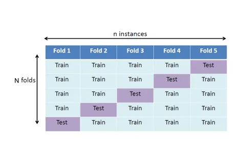
1.4.3 Cross-validation procedures . . . 25

1.5 Contribution of this thesis . . . 26

1.5.1 Microbial identification based on mass-spectrometry data . . . . 26

1.5.2 Jointly learning tasks with orthogonal features or disjoint supports 27 1.5.3 Taxonomic assignation of sequencing reads from metagenomics samples . . . 27

2 Benchmark of structured machine learning methods for microbial identification from mass-spectrometry data 29 2.1 Introduction . . . 31

2.2 Benchmark dataset . . . 32

2.3 Structured classification methods . . . 35

2.3.2 Hierarchy structured SVMs . . . 37

2.3.3 Cascade approach . . . 41

2.3.4 Other benchmarked methods . . . 42

2.4 Experimental setting . . . 42

2.5 Results and discussion . . . 44

2.6 Conclusion . . . 47

3 On learning matrices with orthogonal columns or disjoint supports 49 3.1 Introduction . . . 50

3.2 An atomic norm to learn matrices with orthogonal columns . . . 52

3.3 The dual of the atomic norm . . . 55

3.4 Algorithms . . . 58

3.5 Learning disjoint supports . . . 60

3.6 Experiments . . . 60

3.6.1 The effect of convexity . . . 61

3.6.2 Regression with disjoint supports . . . 62

3.6.3 Learning two groups of unrelated tasks . . . 64

3.6.4 Disjoint supports for Mass-spectrometry data . . . 65

3.7 Conclusion . . . 68

4 Large-scale Machine Learning for Metagenomics Sequence Classifi-cation 71 4.1 Introduction . . . 72

4.2 Linear models for read classification . . . 74

4.2.1 Large-scale learning of linear models . . . 75

4.3 Data . . . 76

4.4 Results . . . 78

4.4.1 Proof of concept on the mini database . . . 78

4.4.2 Evaluation on the small and large reference databases . . . 83

4.4.3 Robustness to sequencing errors . . . 84

4.4.4 Classification speed . . . 86

4.5 Discussion . . . 89

List of Figures

1.1 MALDI-TOF mass-spectrometry. . . 4

1.2 Example of a polyphasic taxonomy. . . 6

1.3 Taxonomic structure of the Tree of Life. . . 7

1.4 Bias-Variance trade-off. . . 11

1.5 Loss functions. . . 13

1.6 Geometry of Ridge and Lasso regressions. . . 15

1.7 Error-Correcting Tournaments. . . 23

1.8 Cross-validation for model selection. . . 26

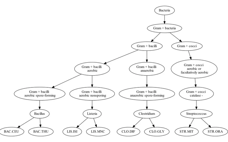
2.1 MicroMass hierarchical tree structure (Gram + bacteria). . . . 34

2.2 MicroMass hierarchical tree structure (Gram - bacteria). . . . 35

2.3 MicroMass dataset visualization. . . 36

2.4 Joint mapping or Multiclass SVM. . . 38

2.5 Joint mapping for Structured SVM. . . 40

2.6 MicroMass dataset: Common classification errors. . . 46

2.7 MicroMass dataset: Mass-spectra clustering at the genus level. 46 3.1 Level sets of the penalty ΩK . . . 51

3.2 The effect of convexity. . . 63

3.3 Sparse regression with disjoint supports. . . 64

3.4 JAFFE dataset: learning curves. . . 66

3.5 JAFFE dataset: correlation in learned models. . . 67

3.6 MicroMass dataset: structured sparsity. . . 68

4.1 From sequencing read to vector space representation. . . 74

4.2 Loss functions and classification strategies. . . 79

4.3 Number of passes during the training step. . . 80

4.4 Features collisions and accuracy in Vowpal Wabbit hash table. 81 4.5 Increasing the number of fragments and the k-mer size on the mini datasets. . . 82

4.6 Large k-mer sizes and collisions in hash table. . . . 83

4.7 Comparison between Vowpal Wabbit and reference methods on the mini datasets. . . 84

4.8 Evaluation on FCP dataset: homopolymer-based models. . . . 87

4.9 Evaluation on FCP dataset: mutation-based models. . . 88

List of Tables

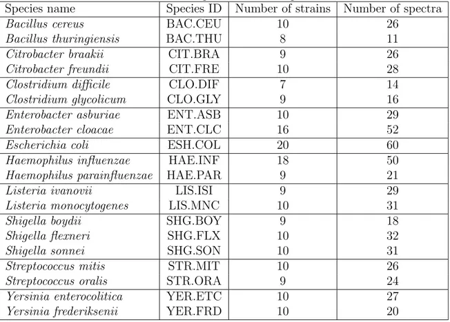
2.1 MicroMass dataset. This table describes the MicroMass dataset con-tent, in terms of used bacterial genera and species. It also provides in-formation on the number of bacterial strains and mass-spectra for each

species. . . 33

2.2 Cross-validation results on MicroMass dataset. . . 44

2.3 Performances of benchmarked methods at genus levels. . . 47

4.1 List of the 51 microbial species in the mini reference database. . . 77

Abstract

Using high-throughput technologies in Mass Spectrometry (MS) and Next-Generation Sequencing (NGS) is changing scientific practices and landscape in microbiology. On the one hand, mass spectrometry is already used in clinical microbiology laboratories through systems identifying unknown microorganisms from spectral data. On the other hand, the dramatic progresses during the last 10 years in sequencing technologies allow cheap and fast characterizations of microbial diversity in complex clinical samples, an approach known as “metagenomics”. Consequently, the two technologies will play an increasing role in future diagnostic solutions not only to detect pathogens in clinical samples but also to identify virulence and antibiotic resistance.

This thesis focuses on the computational aspects of this revolution and aims to contribute to the development of new in vitro diagnostics (IVD) systems based on high-throughput technologies, like mass spectrometry or next generation sequencing, and their applications in microbiology. To deal with the volume and complexity of data generated by these new technologies, we develop innovative and versatile statistical learning methods for applications in IVD and microbiology. The field of statistical learning is indeed well-suited to solve tasks relying on high-dimensional raw data that can hardly be manipulated by medical experts, like identifying an organism from an MS spectrum or affecting millions of sequencing reads to the right organism.

Our main methodological contribution is to develop and evaluate statistical learning methods that incorporate prior knowledge about the structure of the data or of the problem to be solved. For instance, we convert a sequencing read (raw data) into a vector in a nucleotide composition space and use it as a structured input for machine learning approaches. We also add prior information related to the hierarchical structure that organizes the reachable microorganisms (structured output ).

R´

esum´

e

L’utilisation des technologies haut d´ebit de spectrom´etrie de masse et de s´equen¸cage nouvelle g´en´eration est en train de changer aussi bien les pratiques que le paysage scientifique en microbiologie. D’une part la spectrom´etrie de masse a d’ores et d´ej`a fait son entr´ee avec succ`es dans les laboratoires de microbiologie clinique au travers de syst`emes permettant d’identifier un microorganisme `a partir de son spectre de masse. D’autre part, l’avanc´ee spectaculaire des technologies de s´equen¸cage au cours des dix derni`eres ann´ees permet d´esormais `a moindre coˆut et dans un temps raisonnable de caract´eriser `a la fois qualitativement et quantitativement la diversit´e microbienne au sein d’´echantillons cliniques complexes (approche d´esormais commun´ement d´enomm´ee m´etagenomique). Aussi ces deux technologies sont pressenties comme les piliers de futures solutions de diagnostic permettant de caract´eriser simultan´ement et rapidement non seulement les pathog`enes pr´esents dans un ´echantillon mais ´egalement leurs facteurs de r´esistance aux antibiotiques ainsi que de virulence.

Cette th`ese vise donc `a contribuer au d´eveloppement de nouveaux syst`emes de diagnostic in vitro bas´es sur les technologies haut d´ebit de spectrom´etrie de masse et de s´equen¸cage nouvelle g´en´eration pour des applications en microbiologie.

L’objectif de cette th`ese est de d´evelopper des m´ethodes d’apprentissage statis-tique innovantes et versatiles pour exploiter les donn´ees fournies par ces technologies haut-d´ebit dans le domaine du diagnostic in vitro en microbiologie. Le domaine de l’apprentissage statistique fait partie int´egrante des probl´ematiques mentionn´ees ci-dessus, au travers notamment des questions de classification d’un spectre de masse ou d’un “read” de s´equen¸cage haut-d´ebit dans une taxonomie bact´erienne.

Sur le plan m´ethodologique, ces donn´ees n´ecessitent des d´eveloppements sp´ecifiques afin de tirer au mieux avantage de leur structuration inh´erente: une structuration en “entr´ee” lorsque l’on r´ealise une pr´ediction `a partir d’un “read” de s´equen¸cage caract´eris´e par sa composition en nucl´eotides, et un structuration en “sortie” lorsque l’on veut associer un spectre de masse ou d’un “read” de s´equen¸cage `a une structure hi´erarchique de taxonomie bact´erienne.

Chapter 1

Introduction

In this chapter, we provide an overall background and technical notations related to the main concepts studied in this thesis, namely microbiology and supervised learning. Microbiology is the study of all microorganisms and so includes disciplines like bacteriology, mycology or virology. In medical microbiology, the diagnosis of infectious diseases relies on the study of pathogens characteristics. The identification of the infectious agent may involve more than a standard physical examination. For instance, sophisticated techniques (such as polymerase chain reaction [173] or mass-spectrometry [144]) are used to detect abnormalities induced by the presence of a pathogen agent, at a molecular level.

Supervised learning allows to infer a rule between features/measurements and an outcome of interest. This rule is inferred using noisy input observations, called training examples, for which we also know the corresponding output response variable. Once the rule is inferred, it can be used to predict the output of any new input data. For instance, automatic microbial identification based on high-throughput data aims at linking large amount of microorganisms characteristics to their identity, and can be cast as a learning problem. Detailed introduction to supervised learning are given in, e.g, [70, 170].

This chapter is organized as follows. Section 1.1 is related to microbiology and in vitro diagnostics applications. Section 1.2 provides an overview on supervised learning and more precisely on classification in Section 1.3. In Section 1.4, we detail how we correctly compare and evaluate the different methods. Finally, Section 1.5 provides a presentation of the contributions of this thesis.

1.1

Microbiology and in vitro diagnostics

In vitro diagnostics (IVD) tests are comprised of reagents, instruments and systems used to analyze the content of biological samples of interest in the process of a medical diagnosis. For instance, IVD tests are commonly used in a clinical context for measur-ing base compounds in the body, indicatmeasur-ing the presence of biological markers (HIV,

tumor) or detecting disease-causing agents. The same tests are also used for industrial purposes, like food safety or sterility testing, in agri-food, cosmetic, pharmaceutic in-dustries. However, the focus of our research work is restricted to clinical applications. More than 70% of the US medical decisions draw upon the results of an IVD test [66], yet only 2% of the US$2 trillion spent annually on healthcare goes to diagnostics [65]. According to [182], there exists more than 4,000 different tests available for clinical use and about 7 billions of IVD tests are performed each year. They are critical for medical decision-making, allowing to identify infections and diseases, and have a huge impact in terms of lives saved and reduced health care budget thanks to low-cost de-vices for the costly diseases, like cardiovascular diseases, cancer or infectious diseases (HIV, tuberculosis, influenza, etc.)

During my thesis, I spent most of my time working for bioM´erieux, the world leader in IVD tests for microbiology. IVD companies, like bioM´erieux, are massively investing to develop the future diagnostics solutions based on high-throughput technologies.

1.1.1

Diagnostics for infectious diseases

Infectious diseases are caused by pathogenic microorganisms, such as bacteria, viruses, fungi or parasites. Microbial identification, a problematic in IVD, aims at identifying the microorganism causing the disease from clinical samples such as blood, urine or saliva. Identifying a pathogen is a crucial step in the diagnostics workflow and there is still a need for faster and more reliable tests to help clinicians prescribe an appropriate treatment. The other crucial step in diagnostics for infectious diseases is the antibiotic susceptibility testing (AST) [76]. The main goal of AST is to determine which antibiotic treatment will be most successful in vivo. The combination of a correct identification of the pathogen agent and its relevant antibiotic sensitivity represents the ideal clinical therapy. Here, the focus of this thesis is on the development of innovative strategies for microbial identification.

Most existing microbial identification technologies require a culture step. Most bacteria will grow overnight, whereas some mycobacteria require as many as 6 to 8 weeks [13]. Microorganisms present in the sample are isolated on a culture medium that recreates favorable growth conditions. After a few hours, colonies will appear on the medium; each colony only contains replicates of an initially isolated microbe. Thus, this culture step acts like a signal amplification step, multiplying microbiological material in the sample in order to collect enough material from each colony to perform the identification step.

A great variety of identification systems have been proposed, which are sometimes categorized into phenotypic, genotypic and proteotypic methods [160]. Phenotypic methods like, for instance, active pharmaceutical ingredient (API) [4], typically base their identification on the results of several chemical reactions revealing metabolic char-acteristics of the microorganism.

Genotypic identification relies on the genetic material (DNA, RNA) of the microor-ganism and involves sequencing a specific genetic marker, like the 16S rRNA which is often considered as the gold-standard for bacterial identification [46]. These technolo-gies have been commonly used in research laboratories for decades, yet they only started to change the IVD market in the 1990s due to the need for validations [23] by agencies like the US Food and Drug Administration (FDA). The adoption of those complex tests also requires specific training for clinicians and healthcare providers, in particular to in-terpret the results. More recently, so-called proteotypic methods have been introduced as well. These methods base their identification on measurements of the cell content. They include for instance RAMAN spectroscopy [36], fluorescence spectroscopy [21] and Matrix-Assisted Laser Desorption Ionization Time of Flight mass-spectrometry (MALDI-TOF MS) [47].

1.1.2

A new paradigm in microbial identification: high-throughput

technologies

Mass-spectrometry for microbial identification

Until recently, clinical microbiology has mainly relied on conventional phenotypic and biochemical techniques [167]. After a traditional culture step, standardized test sys-tems such as the Phoenix R system (Becton, Dickinson Diagnostics, Sparks, MD), Microscan Walkaway R (Dade-Behring MicroScan, Sacramento, CA), API R and VITEK R 2 (bioM´erieux, Marcy l’Etoile, France), have so far been used to speed up microbial identification: the average time needed for a reliable identification ranges from 6h to 18h [60]. In the last few years, PCR methods have complemented the biochemical approaches, decreasing time-to-results with no mandatory culture step and even be-coming in some cases the reference method [175]. However, PCR methods rely on the design of new oligonucleotide primers requiring the analysis of the genome of each clin-ically relevant microorganism. The efficiency of such approaches can also be reduced by unexpected mutations or unknown variants. Additionally, PCR sensitivity can be too high for some applications, detecting a microbe that is present at non-pathogenic levels [106].

Even if it requires a culture step, MALDI-TOF MS can identify the genus and species of a microorganism after a rapid (few minutes) and simple MS experiment. It is now broadly accepted by the clinical microbiology community as a routine testing tool for microbial identification at the level of species [53,96, 168].

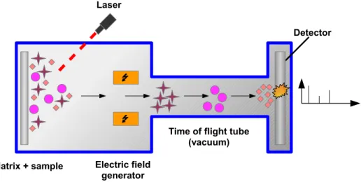
Generally, MS technologies rely on an instrument that takes a sample, ionizes it, for example by bombarding with a laser energy, and converts electric signals to intensity peaks [155]. MALDI-TOF is often referred to as a soft-ionization technology, because of the small amount of energy used, and low risk of bound ruptures. Indeed, fragile biomolecules such as proteins are protected by matrix crystallized molecules from a direct ionization source. Charged particles created by ionization pass through a vacuum

tube playing the role of analyzer. Ions are simply discriminated according to their mass-to-charge ratio (m/z), with a shorter time-of-flight for the smaller ions. At the end of the analyzer, a detector measures, at each impact, the intensity and the mass of the charged particles, leading to an intensity peak profile, also called a mass-spectrum. The whole process is illustrated in Figure 1.1.

Matrix + sample

Time of flight tube (vacuum)

Detector Laser

Electric field generator

Figure 1.1: MALDI-TOF mass-spectrometry. The sample is mixed with a matrix that protects fragile biomolecules. A ionization source, like a laser, is used to pulverized the mixture. Then, ions pass through a vaccum tube where small ions are faster than heavy ones. At the end of the time of flight tube, a detector measures impacts intensity and returns a mass-spectrum profile.

The output of an MS experiment can be represented by a large number of param-eters, like m/z peak positions and their associated intensities. In diagnostic systems based on mass spectra in microbiology, like the Biotyper (Bruker Daltonics, Germany), or VITEK R -MS, the interpretation of raw data is not performed by clinicians, but relies on mathematical algorithms. The major commercially available mathematical systems are the Bruker Main Spectrum analysis (MSP) and the bioM´erieux SuperSpec-trum and Advanced Spectra Classifier (ASC). For those algorithms, the extraction of the intensity peaks and the comparisons of spectra are entirely automated [43]. Each measured spectrum is compared to the spectra in a reference database, and the system converts a similarity score into one or more microbial species names. Indeed, proteins contained in a microorganism are peculiar to their biological species and can be used to identify a microbe observed in a biological sample.

Despite differences in the reference databases, both systems address the large ma-jority of clinically relevant species found in routine clinical practice, including the 20 bacteria that represent > 80% of isolates recovered from human clinical samples. Com-pared to conventional biochemical tests, MALDI-TOF achieves comparable

identifica-tion results for a vast majority (∼ 95%) of the isolates and in case of discordance between the two approaches, 16S rRNA sequencing confirmed MALDI-TOF in 63% of discordant cases [17].

Next-generation sequencing and metagenomics

The study of metagenomes, also called metagenomics, consists in analyzing genetic material recovered from environmental samples. While in traditional microbiology, genome sequencing and genomics rely upon cultivated cultures, metagenomics does not require pure clonal cultures of individual organisms. From an environmental sample, one can estimate its microbial diversity using conserved and universally present markers such as ribosomal RNA [181] and clones specific genes (mostly the bacterial 16S rRNA gene, but 25-30 highly conserved genes are listed in [45]). Such targeted approaches revealed that the majority of microbial biodiversity had been missed by cultivation-based methods [78]. It is estimated that more than 99% of microorganisms observable in nature typically are not cultivable by using standard culture techniques [6, 126].

Recent advances in genome sequencing technologies and metagenome analysis pro-vide a broader understanding of microbes and highlight differences between healthy and disease states. Metagenome studies have recently increased in number and scope due to the rapid advancements of high-throughput Next Generation Sequencing (NGS) technologies such as GS FLX system from 454 Life Sciences, a subsidiary of Roche [112], the IonTorrent’s Personal Genome Machine (PGM) [142], the Illumna MiSeq and HiSeq [19], and the Pacific Biosciences RS (PacBio) [59]. These modern sequenc-ing technologies give us access to a new way of analyzsequenc-ing clinical samples, because they are culture-independent and randomly sequence all microorganisms present in an environment.

1.1.3

Hierarchical organization of microorganisms

Microorganisms are diverse, but share biological properties and evolutionary history. It is therefore useful to group them in a hierarchical structure, called a taxonomy, to organize this diversity. A taxonomic tree is a rooted structure that links groups (taxa) from top and bottom according to general properties (top) to specific properties (bottom): two children taxa sharing the same parent taxon have common features contained in the parent taxon while each sibling taxon has specific characteristics, unshared with its siblings. The taxonomy concept is not proper to the biology field (e.g., semantic Web), but plays an important role in life sciences knowledge organization. Numerous phylogenetic taxonomies are available online, such as NCBI taxonomy [178], UniProt knowledge base [107]. In the in vitro diagnostics context, it is possible to design a polyphasic taxonomic tree as a combination of phylogenetic and phenotypic levels representing successive decision rules used in medical and clinical analysis, as defined for instance in Bergey’s Manual of Bacteriology [74] and shown in Figure 1.2. According

Gram Staining Bacilli, Cocci, ... Anaerobic / Aerobic Family Anaerobic / Aerobic Genus Species

Figure 1.2: Example of a polyphasic taxonomy. Top levels (e.g., Gram stain-ing) correspond to phenotypic classification tests and low levels support phylogenetic information.

to the classification proposed by Carl von Linn´e [104], the finest and lowest level of the taxonomic tree is the species level. The higher ranks are called, from the lowest to the most generic: Genus, Family, Order, Class, Phylum, Kingdom, Domain, as summarized in Figure 1.3. To underline the general character of the higher taxonomic levels, note that there are only three known (and accepted) domains that are Archea, Bacteria and Eukaryota. The last one regroups all organisms made of cells with a genetic material enclosed by a nuclear envelope, including all animals, plants and fungi.

In microbiology, one often considers a level below the species level, called the strain level. A microbial strain is a particular member of a species that differs from the other members by a minor but significant variation [179]. These genetic variations may have a large impact on the expressed characteristics, or phenotypes of the microorganism. For instance, the microbial species Escherichia coli is the most abundant commensal bacteria in the human gastrointestinal track [89] and it coexists with the host with mutual benefit, such as the use of gluconate permease in the colon [161]. However,

Domain Kingdom Phylum Class Order Family Genus Species

Figure 1.3: Taxonomic structure of the Tree of Life. Top levels are the most generic and the bottom levels are the finest.

several E.coli strains have acquired virulence mechanisms allowing a rapid colonization of new environments and causing deadly syndromes, like bloody diarrhea in the recent 2011 E.coli O104:H4 outbreak in Europe [120]. Hence, strains from the same species can have different biological properties related to virulence or drug resistance.

The concept of bacterial species is slightly different from the numerous eukaryota definitions [141], like interbreeding population [115] or other sexual characterizations. The current gold-standard criterion proposed in [122] measures a cross-hybridization proportion between two DNA strands coming from different organisms. The DNA-DNA hybridization (DDH) threshold for considering that two organisms belong to the same species is at least 70%. Because cross-hybridization experiments are not easily applicable to all the bacterial environments, alternative approach based on a conserved gene marker, 16S rRNA, has been proposed in [157]. Results in [93] suggest that a 97% 16S rRNA gene sequence identity is easier to measure with DNA sequencing tech-nologies and is equivalent to the previous 70% DDH threshold. The classification of species has been affected by the gold-standard changes and the technological revolu-tions: from the precipitation assays for blood plasma in 1950’s, to the DDH [150] in the 1970’s, to the recent DNA sequencing. Reorganizations in the phylogenetic taxonomy have been induced at all the classification levels and this tree is still being modified by taxonomists, based on recent findings.

Another issue with the taxonomic organization of the species is the problem of taxa in disguise [87]. They are taxonomic units that have evolved from another unit of similar rank making the parent unit paraphyletic. It means that phylogenetically, all descendants of the parent unit are identical from an evolution point of view but not taxonomically. In general, this paraphyly can be solved by moving the taxon in disguise

under the parent unit. However, in microbiology, reorganizing and renaming taxonomic units may induce confusion over the identity of microorganisms with a medical impact, like pathogens. For instance, the Shigella genus is an “E.coli in disguise” [97] that de-velops a characteristic form of pathogenesis residing on the pInv plasmid [67]. Shigella members are the cause of a severe infectious disease killing hundreds of thousands peo-ple each year: the bacillary dysentery or shigellosis [159]. Because E.coli can also cause similar symptoms, the current taxonomic classification will not change to avoid confu-sion in a medical context. Another example is the species belonging to Bacillus cereus group. They present 16S rRNA sequence similarities around 99-100% [15], higher than the previously described 97% threshold and should be regrouped in a single taxonomic entity. For medical reasons including the pathogenicity of some members, like Bacillus anthracis, responsible for anthrax disease, they will not be merged in the taxonomic tree.

1.2

Supervised learning

Generally speaking, the field of machine learning can be defined as the construction of powerful informatics systems that can learn from observations and measures, instead of following a list of instructions.

In this thesis, we focus on methods for supervised learning. Supervised learning consists in the estimation of a rule between some input and output data. This rule is inferred using noisy observations, called training examples for which we also know the corresponding response variable. The objective is to infer the unknown relation from training data and then, use this rule to correctly predict the output of any new input data. Depending on the nature of the response, one can distinguish two main classes of problem. If the output variable is discrete and represents categories, the problem is called classification, while it is called regression when the response is a continuous real number.

This section first provides general background and notations for supervised learning. Then, we discuss an important concept in learning, the trade-off between approximation and estimation. In the last part of this section, we introduce the regularization concept for learning model under constraints.

1.2.1

Supervised learning: notations

In supervised learning, our goal is to make a model to predict an output Y in an output space Y given an input X in an input space X . The output variable is also often called the response variable. For the output space, we typically take Y = R for regression tasks, or Y = {−1; +1} for binary classification problems. Regarding the input, we will restrict ourselves to data represented by p numerical descriptors or features, hence consider an input space X ⊆ Rp_{. The model is learned from the observation of a set of}

n input-output pairs, (xi, yi)i=1,...,n∈ (X × Y) n

called the training set. For clarity, it is convenient to merge the observed inputs into a n-by-p matrix X = (xi,j)i=1,...n;j=1,...,p,

where each row is an input and each column corresponds to a feature. Similarly, we merge the outputs into a n-dimensional vector Y = (yi)i=1,...,n∈ Yn.

To model the input-output relationship, it is standard in statistical learning to assume that the training examples (xi, yi)i=1,...,n are realizations of random variables

(Xi, Yi)i=1,...,n independent and identically distributed (i.i.d.) according to an unknown

joint distribution P(X, Y ) on X ×Y, and that future observation will also be realizations of independent random variables distributed according to P. Note that this unknown distribution can be written as the product of the marginal distribution P(X), which describes how the inputs are distributed, and of the conditional distribution P(Y |X), which describes how an output is related to an input.

Given a function f : X → Y that deterministically predicts an output f (x) ∈ Y for any input x ∈ X , we would like to measure its quality by how “well” it predicts the response variable on unseen examples. For that purpose, it is useful to introduce a loss function l : Y × Y → R+ to measure the disagreement l(ˆy, y) between a predicted

response ˆy and a true response y, small loss values corresponding to good predictions.

We will discuss in more details standard loss function in Section 1.2.3. Given a loss function, the risk of a predictor f : X → Y can now be defined as the expected loss it will incur on unseen examples, namely

R(f ) =

Z

l(f (X), Y )dP(X, Y ) . (1.1) The goal of statistical learning can then be summarized as the task of using the training set to estimate a predictor ˆf : X × Y with the smallest possible risk R( ˆf ).

1.2.2

Empirical risk minimization, approximation and

estima-tion errors

Ideally, the goal of statistical learning is therefore to find the predictor f∗that minimizes the risk R(f ) over all possible measurable functions f : X → Y, by solving the risk functional minimization problem [169]

f∗ = arg min

f

R(f ). (1.2) Unfortunately, since the joint probability P(X, Y ) is unknown, the risk R(f ) is not computable and f∗ is not reachable. Instead of R(f ), what we can compute from the training data is the empirical risk :

Remp(f ) = 1 n n X i=1 l(f (xi), yi) , (1.3)

which for each f is an unbiased estimate of R(f ). To estimate a predictor ˆf from the

training data, the empirical risk minimization (ERM) estimator is the predictor that minimizes the empirical risk over a pre-defined set of candidate predictors F :

ˆ

f = arg min

f ∈F Remp(f ).

(1.4)

The choice of the set of candidates F is of uttermost importance for learning. Roughly speaking, if F is too large, for example if we consider all possible measurable functions, then we may find complicated functions (in fact any function passing through all the points in the training set) with minimal empirical risk, which may however make terrible predictions on unseen examples. This phenomenon is called overfitting, and can be controlled by reducing the set of candidates F . On the other hand, if F is too small, then it may be the case that no predictor in F is a good model for the input-output relationship, leading to poor predictors too. This situation is called underfitting. To characterize the role played by F in controlling overfitting, it is useful to decompose the excess risk of ˆf compared to the optimal risk of f∗ as follows:

R( ˆf ) − R(f∗) = [R( ˆf ) − min

f ∈F R(f )] + [minf ∈FR(f ) − R(f

∗

)] (1.5) = estimation error + approximation error. (1.6) Here, the estimation error is due to the difficulty of approximating the true risk by the empirical risk with a limited amount of training data, while the approximation error is induced from approximating f∗ with a restricted model space F that does not necessarily contain f∗. Intuitively, this error decomposition is similar to the classical bias-variance trade-off with the estimation error playing the role of the variance and the approximation error playing the role of bias. In this setting, a model selected in a restricted set F does not fit the data well and is biased. On the other hand, a model selected on a complex and large set of functions does not generalize its predictions if small changes to the data distribution occur: this is a high-variance solution. Figure 1.4 illustrates the evolution of training error (red) and generalization error on new data (blue), as functions of the estimated model complexity. The error on the training data can always be decreased by using complex models that overfit the dataset, inducing poor generalization performances. We represent with a black dot, the optimal model in the sense that it minimizes the test error which is our goal. With high-dimensional data, the estimation error can easily dominate the approximation error if F is not drastically controlled. This explains to some extent why simple models such as linear predictors are popular and successful in many applications of machine learning, and are the standard models in many algorithms such as linear regression, logistic regression, or support vector machines [50].

Model complexity Prediction error ● Low High Train error Test error

Figure 1.4: Bias-Variance trade-off. The prediction error on the training data (dotted red line) monotonically decreases with more complex models. For those models, the error made on new data (blue) illustrates the problem of overfitting with high error values for “too complex” models. An optimal model in terms of a trade-off between bias and variance could be the one with the minimal generalization error (black dot).

1.2.3

The choice of a loss function

The definitions of the risk (1.1) and of the empirical risk (1.3) depend on the choice of a loss function l, which we now discuss. Perhaps the most intuitive notion of risk, particularly for classification problems, is to count the number of mistakes made by the model when predicting outputs for new data. The corresponding loss function is called “gold-standard” or “0-1” loss and can be formulated as follows

l0−1(y, f (x)) =      0 if f (x) = y, 1 otherwise.

Although this loss function is intuitively appealing, it is rarely used because it leads to computationally difficult optimization problems when we want to solve the empirical minimization problem (1.4), due to its non-convexity. Instead, it is common to con-sider convex surrogate loss functions, which lead to empirical risks which are convex functionals of f and can efficiently minimized. Remember that a function h : Z → R

over a convex set Z is convex if [137]

∀z1, z2 ∈ Z, ∀t ∈ [0, 1] : h(tz1+ (1 − t)z2)) ≤ th(z1) + (1 − t)h(z2). (1.7)

In the case of binary classification (Y = {−1, +1}), the hinge loss is defined as

lhinge(y, f (x)) = max(0, 1 − yf (x)). (1.8)

It is a convex loss used in particular in the support vector machine algorithm [50]. More details are given in Section 1.3.1.

Another convex loss function, commonly used in classification, is called logistic, because its empirical risk is linked to the log-likelihood of the logistic regression. It is defined as

llog(y, f (x)) = ln(1 + exp(−yf (x))). (1.9)

The hinge and logistic loss functions are convex surrogates for the l0−1 function in

binary classification. For regression (Y = R), let us mention the popular squared error loss function, because of its importance in linear regression problems, such as least squares regression. It is defined as

lsquared(y, f (x)) = (y − f (x))2. (1.10)

Note that the squared error loss can also be used in classification settings, for example, by rounding an estimated output to its closest integer.

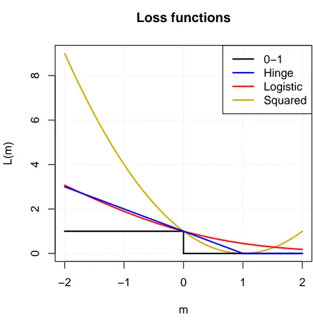
Figure 1.5 shows the four loss functions described, as a function of the margin

m = yf (x). Apart from the squared loss which is clearly different, the hinge and

logistic loss functions behave as convex versions of the 0-1 loss. We also note that the logistic loss is softer than the hinge loss which is non-differentiable for yf (x) = 1.

1.2.4

Regularized methods and model interpretability

In Section 1.2.2, we explained the need to restrain the set of candidate functions F in order to avoid overfitting and balance the estimation and approximation errors. We also mentioned that linear predictors are frequently used in machine learning problems, for their simplicity and performance. For that reason, we consider these models in the following sections. Formally, a function f (x) is a linear function of x = (x1, . . . , xp) ∈

Rp if it can be written as fw(x) = w>x = p X i=1 wixi

for a weight vector w ∈ Rp_{. In this setting, the empirical risk minimization problem}

(1.4) is equivalent to

ˆ

w = arg min

w∈W Remp(fw

−2 −1 0 1 2 0 2 4 6 8

Loss functions

Figure 1.5: Loss functions. The squared (gold), logistic(red), hinge (blue) and 0-1 (black) losses are depicted in this figure.

where the set W is a subset of Rp. A standard way to define W is through a penalty/regularizer function Ω : Rp → R, as follows:

ˆ

w = arg min_w∈RpRemp(w)

s.t. Ω(w) ≤ µ , (1.12)

where µ ∈ R+. Interestingly, under weak assumptions on the convexity of the loss

function l and of the penalty Ω, the Lagrange multiplier theory [25, Section 4.3] tells us that if ˆw is the solution of (1.12) for a certain µ > 0, there exists λ ≥ 0 such that

ˆ

w is also a solution of the regularized problem:

min

w∈RpRemp(w) + λΩ(w). (1.13)

This result allows some flexibility in the way to present the problem (1.11): the con-strained and the regularized formulations. Even if there is no direct mapping between the two constants µ and λ, they play an inverse role in the regularization of w. When

µ = +∞ (resp. λ = 0), there is not constraint on w and W = Rp_{. On the contrary, if}

µ = 0 (resp. λ = +∞), the only feasible solution is the zero vector. In the following

w, such as smoothness, sparsity, or more complex structured constraints.

Rigde regression

We recall that the least squares estimator which minimizes

min w∈Rp 1 2 n X i=1 (fw(xi) − yi) 2 = min w∈Rp 1 2kY − Xwk 2 2

is given by (X>X)−1X>Y, and that the problem is ill-posed when p > n in the sense that it has multiple solutions. Ridge regression was proposed by [72] to solve the least squares problem when p > n, by adding a `2-norm penalty to the standard least squares

problem: ˆ w = arg min w∈Rp 1 2kY − Xwk 2 2+ λ 2 p X i=1 w_i2. (1.14)

The solution of the problem (1.14) is indexed by the regularization parameter λ and is now seen to be

ˆ

wridge= (X>X + λIp)−1X>Y, (1.15)

where Ip denotes the identity matrix in Rp×p. Although the main motivation for ridge

regression was historically to reduce numerical issues when inverting X>X by adding a positive ridge on the diagonal of the matrix, it is also beneficial for statistical reasons by controlling the estimation/approximation error balance with the penalty function Ω(w) = kwk2

2. This regularization has also been applied to classification learning tasks

with other loss function, like support vector machines in the case of the hinge loss [50].

Sparsity-inducing penalties

The trade-off between model complexity and its generalization to new data has also been studied through feature selection and sparse models, that is, by estimating pre-dictors that only take into account a subset of the features. Sparse models are popular because the selection of a smaller feature set can make the model more interpretable, but also because constraining a model to use only a limited number of features is a way to fight overfitting by controlling the complexity of the class of candidate models. A popular formulation to infer sparse linear models in a computationally efficient frame-work is the Least Absolute Shrinkage and Selection Operator (Lasso) method [165], which is similar to the ridge regression (1.14) but regularizes the squared error by an

`1-norm regularization instead of an `2-norm:

ˆ

wLasso= arg min

w∈Rp kY − Xwk2₂+ λ p X i=1 |wi|, (1.16)

where λ ≥ 0 and |.| denote the absolute value function. Like for ridge regression, the Lasso solution converges to the least squares solution when λ goes to zero. Figure 1.6

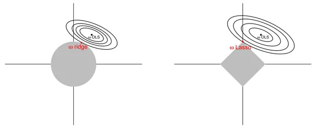
shows the Ridge (left) and Lasso (right) geometrical interpretations in dimension 2. In each panel, the grey region corresponds to the constraint set {kwk ≤ 1} and the ellip-tical contours are the least squares error for different solutions. The optimal solution of the constrained problem is represented with a red dot, as the first contour meeting the constraint set. For the Lasso regression, the diamond shape of the constraint set leads to a solution at a corner, where the first coordinate w1 is equal to zero, while it

can not be the case for the ridge regression, due to its circular shape.

● ω OLS ● ω ridge ● ω OLS ● ω Lasso

Figure 1.6: Geometry of Ridge and Lasso regressions. Left: the Ridge constraint

w2

1 + w22 ≤ 1. Right: the Lasso constraint |w1| + |w2| ≤ 1. The elliptical contours

rep-resent some residual sums of squares. the minimization of the residual sum of squares according to the constraint corresponds to the contour tangent to the grey shape. In the Lasso case, the solution (red) occurs sometimes at a corner and corresponds to a zero coefficient in w (here, the first coordinate).

Although Lasso is performing optimally in high-dimensional settings [22], it is known to have stability problems in the case of strong correlations between the fea-tures [186]. For instance, the Lasso will randomly select one variable among a group of highly correlated variables.

Recently, many methods have been proposed to incorporate more information about the underlying structure linking the variables. To name a few, the elastic net [186] combines the `1 and `2 norms to ensure the joint selection of the correlated features,

but does not explicitly take into account the actual correlation structure if it is known. The group Lasso [185] and its overlapping version [81] consider pre-defined subgroups of features and regularize the sum of the `2 norms of these groups. These approaches

require a prior knowledge on the groups composition. If the correlation structure is suspected but unknown, the k-support norm was proposed by [9] as an extension of the elastic net, that consider all the possible overlapping groups of size k.

orthogonal or disjoint groups of features through multiple classification tasks.

1.2.5

Solving the empirical risk problem

The empirical risk minimization problem (1.4) aims to find a model w that minimizes the average loss on the training examples. In this section we discuss practical algorithms to solve this problem, when the loss function is convex. While any convex optimization problem may in theory be solved by general-purpose techniques like interior point methods, such techniques are computationally heavy in high dimensions and first-order methods such as gradient or stochastic gradient techniques are often preferred in machine learning. For simplicity, we consider unregularized problems where Ω ≡ 0 in this section, the extension to regularized problem being relatively straightforward [147].

Gradient descent (GD)

In order to solve this optimization problem, several papers, like [143], proposed a gradient descent minimization. Considering that the gradient of the empirical risk (1.3) is available for each training point, each iteration updates the weight vector w from the previous step:

wt+1:= wt− γt n n X i=1 ∇wl(wt>xi, yi), (1.17)

where γt is a constant or decreasing parameter. Results in [55] demonstrate that,

under conditions on the starting point w0 and the choice of γt, this algorithm can

achieve linear convergence rates to the optimum (i.e., the distance between wt and

w∗ decreases like exp(−t)). Although the convergence is slower than second-order methods like Newton-Raphson in terms of number of iteration, first-order methods that only require a gradient estimation at each iteration are faster in practice.

Stochastic gradient descent (SGD)

Stochastic Gradient Descent can be thought of as a simplification of classical gradient descent, particularly useful when the number of training examples n is very large [26]. Indeed, in the gradient descent scheme, each iteration (1.17) relies on the computation of an average value over all the examples taking a time proportional to n, which can be prohibitive when n is very large. At each iteration, SGD estimates the gradient using a single and randomly picked example instead of computing a gradient on the whole training set:

wt+1:= wt− γt∇wl(wt>xt, yt), (1.18)

where (xt, yt) is the training point randomly picked at the step t. Very often, the

Those cycles are also called passes or epochs.

In terms of convergence speed, this approach is slower than the classic gradient descent with a convergence speed in 1_t at best [101]. Intuitively, SGD is able to converge as fast as gradient descent to an optimal neighborhood, but the gradient estimation on a single training point induces some variations around the optimum. However, each SGD iteration is very fast and efficient to implement, since it only requires looking at one training point at a time. In addition, the large amount of data available in many domains (e.g., health care, public sector administration, personal location data,...[111]) keeps increasing and some recent works (e.g., [131]) even consider that the training set is virtually infinite. In this setting, on-line learning algorithms consider the training set as a data streaming and perform a single pass over the available examples. With a infinite number of examples and an allowed training time tmax, one can run SGD on as

many training points as possible before the imparted time, or one can select a subset of the training set that can be processed by a standard gradient descent, in memory and time. Theoretical results proposed in [28] indicate that the most efficient option is to use the maximal number of different examples with an on-line algorithm. Indeed, even if the convergence of the GD algorithm is better than SGD, the total number of examples considered by SGD will be higher than GD. Interestingly, considering a infinite training set is equivalent to drawing the examples according to the unknown probability distribution P(X, Y ). So, instead of minimizing an empirical risk Remp with

a finite training set, the on-line learning algorithm will directly minimize the expected risk R. We refer the interested reader to a detailed study of the GD and SGD properties [27].

1.3

Classification

In this section, we continue our introduction to machine learning with a particular focus on classification problems, and review in particular various techniques that implement or not the regularized empirical risk minimization principle.

1.3.1

Binary classification

We first consider the simple case of discriminating only two classes, meaning that the output space Y is restrained to {−1, +1}. The goal of binary classification is to find a decision rule which may be used to separate the inputs Xi belonging to the different

class labels Yi. This can be interpreted as computing the posterior probabilities p(y|x)

for y ∈ {−1, +1} and choosing the maximal value. Fisher Linear Discriminant

The Fisher Linear Discriminant described in [124] is one of the simplest classification algorithms. The idea is to find the best direction w which maximizes the interclass

variability and minimizes the intraclass variability. The variability between the classes

SB is defined as (µ−1− µ+1)(µ−1− µ+1)>, where µ−1 (resp. µ+1) is the mean value for

the class “-1” (resp. class “+1”). The variability within the classes SW is defined as

SW = X C∈−1,+1 X i∈C (xi− µC)(xi− µC)>. (1.19)

Finding the optimal direction w is equivalent to solve the following problem

ˆ w = arg min w∈Rp w>SBw w>_S Ww , (1.20)

which can be computed by using a simple procedure based on the Lagrangian formu-lation. To predict a new data point with Fisher Linear Discriminant, one calculates the distance from the point to the means of the projections of the training classes on the direction ˆw and returns the closest class. There is also a weighting scheme that

minimizes the bias induced by unbalanced training classes.

k Nearest Neighbours

The k Nearest Neighbours (k-NN)[51] relies on a more local classification than the Fisher Linear Discriminant. A new data point is classified according to the predomi-nantly represented label in a neighbourhood of size k. The k closest neighbours depend of the choice of a suitable distance, which by default it often the Euclidean distance.

Nearest Prototype

In the presence of a large training dataset, computing all the distances between a new point and the training examples can be computationally expensive for the k-NN algorithm. An alternative proposed in [42] and called Nearest Prototypes consists in summarizing each class label by a small subset of training points: the prototypes. It is also possible to define a class centroid as the average prototype (Nearest Centroid approach). Here, the classification of a new data point only requires the computation of a distance value per class.

Decision tree

The Decision Tree method [33] constructs a tree structure by recursively separating the training points in subsets. In each non-terminal node, the algorithm determines, on the subset of training data affected to this node, a decision rule of the form Xi < ci,

where Xi corresponds to a particular variable describing the input data and ci is a

constant threshold value. There also exists some extensions that consider decision rule with linear combinations of the input variables, instead of a single variable. Based on this rule, each training point can be affected to one of the two children nodes, until it comes to a leaf node, where the prediction is made. The optimization of each decision

rule generally relies on a criterion which maximizes the homogeneity within each child node and the heterogeneity between the two children nodes. Let us introduce some more notations to described such criteria. We denote by Nm the number of training

observations affected to the node m, by Rm ⊂ Rpthe subspace described by the decision

rule at the node m, and by pmk, the proportion of training points belonging to the class

k and affected to the node m: pmk = 1 Nm X xi∈Rm I(yi = k). (1.21)

The predominantly represented class in the node m is denoted by k(m) = arg max_kpmk.

The main criteria used to optimize the decision rules at each node include: • Misclassification error: 1 Nm X xi∈Rm I(yi 6= k(m)) = 1 − pmk(m) • Gini index [63]: X k6=k0 pmkpmk0 = K X k=1 pmk(1 − pmk) • Cross-entropy/deviance:− K X k=1 pmklog pmk. Random Forests

Random forests [32] is a learning method that combines multiple decision trees. For each tree construction, a subset of training examples is randomly sampled, as it is done in Bagging [31], and considered as the new training set for this tree. In addition, the cut at each node is usually optimized over a random subset of the features. For the prediction of a new data point, the data is passed through all decision trees, each voting once, and the output is the most popular class.

Naive Bayes Classifier

A Naive Bayes (NB) classifier is based on applying Bayes’ theorem assuming that all features in the input space are independent of each other. To label a new data point x, the posterior probability of class Ci ∈ {−1, +1} given x is P (Ci|x). The decision rule

of the Bayes classifier is to choose the class ˆC, with the largest posterior probability.

ˆ

C = arg max

i

P (Ci|x). (1.22)

Applying the Bayes rule, the posterior probabilities P (Ci|x) can be calculated by:

P (Ci|x) =

P (x|Ci) × P (Ci)

P (x) , (1.23)

where P (x|Ci) is the probability of observing x in the class Ci, P (Ci) is the prior

x. Because P (x) is the same for each Ci, the problem (1.22) is equivalent:

ˆ

C = arg max

i

P (x|Ci) × P (Ci). (1.24)

Assuming conditional independence between each feature, the class-conditional proba-bility is the product of p individual probabilities:

P (x|Ci) = p

Y

j=1

P (xj|Ci). (1.25)

In the case of discrete features (like the ones in document classification), those individ-ual probabilities P (xj|Ci) correspond to the maximum-likelihood solution of a

multi-nomial model [132] and are typically estimated by counting the overall proportion of each feature xj in the Ci class members:

P (xj|Ci) =

#{xj ∈ Ci}

#{x ∈ Ci}

. (1.26)

Generally, one estimates P (Ci) as the proportion of examples belonging to the class

Ci in the training set. Under the assumption that all (P (Ci))i are equal, the scoring

function (1.24) can be simplified : ˆ C = arg max i p Y j=1 P (xj|Ci). (1.27)

Support vector machine (SVM)

SVM have met significant success in numerous real-world learning tasks, including text classification [50,85]. In its original form, the SVM algorithm is a binary classification algorithm. It aims at building a classification rule allowing to classifying instances from a space X as positive or negative. In other words, the SVM algorithm seeks to build a hyperplane separating the space X in two half-spaces. In the following we will consider the usual case where X is a standard Euclidean vector space, but we note that SVM can be generalized to non-vector spaces (e.g., sequences or graphs) using kernels [3]. To learn the function f , the SVM algorithm seeks to correctly classify the training data while maximizing the margin of the hyperplane, which is inversely proportional to the norm of the vector w. These two criteria are hard to fulfill simultaneously, and in practice the SVM algorithm achieves a trade-off between these two objectives. This trade-off is controlled by a parameter usually denoted as C, and the SVM solution is

obtained by solving the following optimization problem: min w,b,ξ 1 2kwk 2_{+ C} n X i=1 ξi (1.28) such that : (1.29) ξi ≥ 0, ∀i (1.30) yi(hw, xii + b) ≥ 1 − ξi, ∀i, (1.31)

where (ξi)iare called slack variables and take values greater than 1 only for misclassified

points. The standard SVM formulation is a regularized problem (1.2.4), where the penalty is the `2-norm and the loss function is the hinge loss. The C parameter plays

the same role as 1/λ.

In Chapter 2, we describe more complex and structured SVM formulations em-bedding a regularization based on a hierarchical tree distance between the different classes.

1.3.2

Multiclass extension

One may consider a more complex case, where the possible affectations for a input

x belong to an extended set of labels Y = {1, ..., K} Interestingly, all the previously

described approaches can be extended to the multiclass case [5]. In some cases, like for example for k-NN or decision tree classifiers, this extension is natural and simply replacing the set of labels {−1, +1} by 1, ..., K is sufficient. In other cases, some specific strategy must be implemented, as summarized in the rest of this section.

Multiclass SVM

For the SVM approach, reformulations of the binary problem (1.28) have been proposed to handle the multiclass case [176,30, 52, 166]. However, the formulations in [176,30] result in a single constrained problem that can be unfeasible for a large K, while those in [52,166] are more efficient for a large number of classes. These approaches generally learn simultaneously a set of class specific weight vectors wk ∈ Rp, for k = 1, ..., K. To

do so, the idea is to learn the weight vectors from the training dataset such that the highest scores are given by the scoring functions of the appropriate class. Formally, we want to achieve the following criterion:

hwyi, xii ≥ hwk, xii for k ∈ Y \ yi, and i = 1, ..., N,

where “\” is the set exclusion operator. To efficiently solve this problem, we adopt a SVM-like formulation where we enforce a margin in the above constraints

but tolerate margin violations

hwyi, xii ≥ hwk, xii + 1 − ξi with ξi ≥ 0, for k ∈ Y \ yi.

Altogether, this gives the following optimization problem [52]:

min {wk}k=1..K,ξ 1 2 K X k=1 kwkk2+ C n X i=1 ξi (1.32) such that : (1.33) ξi ≥ 0, ∀i (1.34) hwyi, xii ≥ hwk, xii + 1 − ξi, ∀i, ∀k ∈ Y \ yi. (1.35)

Note that the prediction step uses the decision rule ˆC(x) = arg max_khwk, xi.

This extension of the binary SVM to a multiclass setting requires to change the original formulation and in some cases, there is no evidence that a single mathematical function correctly separates all the represented classes [2]. Furthermore, the most standard and easiest way to address multiclass classification problems with SVMs is to combine binary classifiers into a multiclass classification rule, as explained below.

One-versus-all (OVA)

The one-versus-all scheme [135] consists in learning a set of K binary SVMs trained to separate each of the K classes from the K −1 other ones, leading to a set of hyperplanes

n

wk

o

k=1,...,K, and the class predicted for the instance x is the one obtaining the highest

score, as in the multiclass formulation. Compared to the multiclass scheme, we end up with K problems instead of a single optimization problem, with however a lesser number of constraints than the unique multiclass problem. The benefit that can be expected by the multiclass formulation with respect to the OVA scheme is to obtain better classification performances due to a better calibration of the K scoring functions used to make the prediction. Indeed, in the one-versus-all scheme, no mechanism explicitly enforces the scoring functions of a given class to be higher to those of other classes (and in particular to similar ones). However, [136] provides performances comparable to multiclass approaches.

One-versus-one (OVO)

The one-versus-one scheme [69] is also called pairwise classification. A set of K(K − 1) 2 binary SVMs is trained to distinguish between every pair of classes, and the class predicted for an instance x is the one obtaining the highest number of votes (a number between 0 and K − 1) according to these classifiers. Results in [75] suggest that this approach can perform better than the OVA formulation.

Error-Correcting Output-Coding (ECOC)

This approach uses the concept of error-correcting codes detailed in [56]. It works by training a fixed N number of binary classifier that is greater than K. Each class is then represented by a different binary code of length N . The class codes can be summarized in a binary matrix in {0, 1}K×N_{, where each row is a class code. For each column of}

this matrix, a classifier is learned using the zero-labeled classes as negative examples and the other ones as positive examples. The label prediction of a new data point is done by putting the N predictions into a binary code and by returning the closest class in terms of Hamming distance [68] between the class codes and the predicted code. Results reported in [56] show a better generalization ability of ECOC over the OVA and OVO formulations.

Error-Correcting Tournaments (ECT)

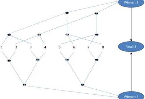
The multiclass formulations presented above have a running time which is O(K) [135] and does not scale very well with large K classification problem. An alternative to these strategies is described in [20] and is called Error Correcting Tournament (ECT). This approach operates in two phases, described in the Figure 1.7. The first step consists in

m single-elimination tournaments over the K labels. For each tournament, labels are

paired at the first round and the winners of each round play a second round, and so on. At the end of a tournament, there is a single winner: the predicted label for this tournament. Then, given the m predicted labels, there is an “All-Star” tournament in order to decide which winner label is the final prediction returned by the algorithm.

1 2 3 4 5 6 7 8 1 4 6 7 7 6 4 1 1 4 4 6 Winner: 1 Winner: 4 Final: 4

Figure 1.7: Error-Correcting Tournaments. This is an example of m = 2 elimi-nation tournaments with K = 8 classes. Each tournement has its own tree structure, leading to different winners for the same data point ot classify. A final round between the different tournaments winners allows to select the predicted label.

Interestingly, this approach provides a complexity for training and test steps in O(log(K)) which is well suited to classification problems with large number of classes. As a side effect, the gain in computation speed for ECT is counterbalanced by decreas-ing accuracy performances [44].

However, there is no clear evidence that, in general, a formulation is better than the others. This suggests that the best multiclass strategy is problem dependent.

1.4

Model evaluation

In order to efficiently compare the different machine learning approaches, one needs standard evaluation rules. In this section, we describe some of them that are used in the next three chapters. As stressed in Section 1.2.2, a good predictive model should demonstrate high generalization on a new data set.

1.4.1

Accuracy measures

Let us assume that we have a so-called test set of n input-output pairs that was not used to train a predictor ˆf . Here we discuss how it can be used to estimate the performance

of ˆf on future data.

The performance indicators we consider obviously depend on the learning task. In a regression context, like in Section 3.6.1, we can compute the average l2 loss error,

also called Mean Squared Error (MSE)

MSE(Y, ˆY ) = 1 n n X i=1 (ˆy − y)2, (1.36) where Y = (y1, ..., yn) is the vector of actual responses and ˆY = (ˆy1, ..., ˆyn) is the vector

of values estimated by the predictive model.

For the classification tasks evaluation, we may consider several indicators. First, a common measure is the correct classification rate, also called micro accuracy [146,110]. It is defined as the proportion of correctly labeled examples for a given dataset and directly involves the “0-1” loss

1 n n X i=1 I(ˆyi, yi), (1.37)

where I is the indicator function equal to 1 if the compared terms are equal and 0 otherwise. In the multiclass classification context, unbalanced class sizes may induce a bias in the micro-accuracy score: large classes dominate small classes in the overall correct classification rate. To put similar weights on small classes, [110] proposed a macro accuracy score

1 K X c∈C 1 Nc X i∈c I(ˆyi, yi), (1.38)