An Energy Efficient Autopilot Design

Journal of Sailing Technology 2020, volume 5, issue 1, pp. 1 - 19. The Society of Naval Architects and Marine Engineers.

An Energy Efficient Autopilot Design

Madintec/Université de Bretagne Sud, France, mathilde.trehin@univ-ubs.fr.

Johann Laurent

Université de Bretagne Sud, Lab-STICC UMR6285, France.

Hugo Kerhascoët

Madintec, France.

André Rossi

Université Paris-Dauphine, LAMSADE UMR7243, France.

Jean-Philippe Diguet

CNRS, Lab-STICC UMR6285, France.

Manuscript received July 14, 2019; revision received November 14, 2019; accepted December 12, 2019.

Abstract. In this paper, we propose a new control method for the next generation of sailboat

autopilots. These new systems will need to manage more actuators to control the hydrofoils, which is going to significantly increase the energy requirements. So, this method is aware of the autopilot power consumption. It uses a model predictive controller to manage the actuators. This controller uses a dynamic model of the actuator, running in real time, to anticipate the future behavior of the system. Once the predictions are made, it determines the future control sequence to apply in order to follow the reference trajectory. To do so, it minimizes a cost function which takes into account two criteria: the precisionof the system and the energy. With the proposed control method, skippers can focus on one or the other criterion depending on their goals and the boat’s energy balance. We apply this method to one of the autopilot’s subsystems, namely the rudder control. The electric actuator intervening in this control loop and the load representing the force opposed to its motion are modelled to design the control law. The first results of that method are compared with a standard autopilot. We increase by 40% the precision level and we are able to reduce the consumption by at least 20%. This work provides the first necessary components of a future

autopilot that will control the whole appendages to a three-dimensional piloting. Moreover, this type of management is a first step towards possible fossil fuel-free sailboats.

Keywords: Automation; electronics; navigation; sailing; systems engineering. NOMENCLATURE

𝐶_"#$ Resistive torque [N m] 𝐸 Span [m]

e Planform efficiency factor (Oswald coefficient) [-] 𝐹_'()"* Hydrodynamic force [N]

𝐹+ Lift force [N]

𝐹_"#$ Resistive force [N] 𝐹- Drag force [N]

𝑖 Electric current [A]

𝑘₀ Proportional coefficient [-] 𝐿 Motor inductance [H]

𝑁+ Prediction horizon [-] 𝑝 System input [-] 𝑄5, 𝑄7 Load factor [-] 𝑅 Motor resistance [Ω] 𝑆 Surface [m2_] 𝑢 Voltage [V]

𝑉 Speed of the incident stream [m s-1_]

𝜗 Linear speed [m s-1_]

𝑥(𝑘) System state [-] 𝑦 System output [°] 𝑦_" System set point [°] 𝛼 Angle of attack [rad] 𝛾 Linear acceleration [m s-2_]

𝛿 System precision [°] 𝜀 Precision constraint [°] 𝜃̇ Rotation speed [rad s-1_]

𝜆 Aspect ratio [-]

𝜌 Water density [kg m-3_]

MPC Model Predictive Control PID Proportional Integral Derivative LQR Linear Quadratic Regulator

1. INTRODUCTION

Over the years, the sailboats designed for ocean races have evolved a great deal in order to gain in performance. The hulls changed to get more powerful profiles and are now composed of the latest-generation composite materials. Foils equip them and thanks to these improvements, the sailboats, initially in a displacement mode, became “flying machines”. Embedded systems are part of these most recent technological developments and evolve into key components to optimize the boat settings (Douguet 2013). They already use and analyze more than one hundred data sensors and are becoming increasingly complex under great performance and safety pressure.

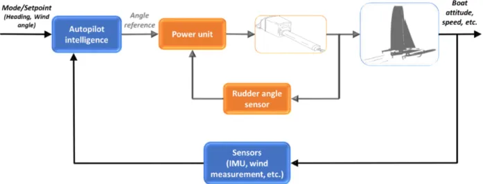
For example, the autopilot, which is basically a control process running on a microcontroller, assists the skipper to steer the sailboat more than 95% of a solo race. Thanks to the autopilot system, the skipper can focus all his/her attention on sail trim and free up more time to refine tactical elements or for media communications. So, it has become an indispensable element of a solo race. An autopilot is composed of two control loops, the heading/attitude control and the rudder angle control (Figure 1).

To enable a quasi-permanent use of the autopilot, the system needs a reliable energy supply around the clock. However, energy resources are limited on board. They have a few renewable energy producers (solar panel, wind turbine, etc.), but they can meet the boat needs only under specific weather conditions. They have a finite quantity of fuel that can recharge a battery set but they try to gain in performance by minimizing the weight which means reducing the fuel volume. With the arrival of the new hydrofoil sailboats, the next generation autopilot will need to manage more actuators to control all these appendages. It is going to increase the computing and energy requirements. So, taking into account the energy criterion in the control laws and optimize its use is becoming mandatory to increase the number of managed actuators, to move towards a sailboat without fossil fuel and to guarantee skipper safety.

Figure 1: Autopilot control loops

Currently, the methods available in the scientific literature don’t pay attention to the autopilot power consumption (Shi et al. 2017; Tomera 2010). They focus only on the boat performance and safety by improving the reactivity, the robustness or the adaptability of the system in a complex

environment. As seen previously, to be able to manage the new hydrofoil sailboats, what is really needed is an autopilot which can adapt its control law to the energy constraints linked to the offshore sailing race environment. So, in this paper, we propose a new control method aware of the autopilot power consumption.

The first section includes a set of today’s autopilot control laws. The second section explains our control method which is aware of the power consumption, its principle and setting up. In the last section, the rudder control case study is entirely detailed (models, control tuning and results). Finally, a summary of the main concepts of the paper and a concise presentation of the future prospects end this document.

2. AUTOPILOT CONTROL LAWS

Many laws exist in the field of drive control and a lot of them have been tested for autopilot systems. Some of them are presented in this section.

2.1. In the sailboat industry

According to some skippers’ feedback about the autopilots currently on the market, it is regularly necessary to adjust the gains/settings in function of the sailing conditions. In fact, the implemented control laws used in the sailing domain remain quite simple and only one tuning can’t adapt to every sailing condition. These are usually PID controllers. As a reminder, a PID controller

(Proportional Integral Derivative) acts in function of the error value as the difference between a set point and a measured signal. It applies a correction based on Proportional, Integral and Derivative terms (Figure 2). So, this method is based only on measuring and calculating the error and not on the knowledge of the system behavior. It can perform well within some industrial environments and appears to be conceptually intuitive but its tuning can be difficult if opposing objectives such

reactivity and high stability are to be achieved (Ang et al. 2005). Some PID configuration methods exist (Ziegler-Nichols, Nyquist, etc.) but they can be difficult to apply to a sailboat because they need to have an observation and a characterization of the system answer to an excitation. Moreover, the boat operates in a complex and uncertain environment, the skipper often needs to modify the controller gains in navigation to match the sailing conditions.

Figure 2: PID controller

The autopilot control is a complex problem and various scientific studies looked into the problem to improve it. The next section details some of them.

2.2. In the areas of research

Most of the scientific studies focus on ships or sailing robots which don’t have the same steering responses under stress. Only a few are interested in the sailboat, a complex system severely disrupted by the two uncertain environments where it operates, water and air environments. A significant part of these studies tries to reproduce the human behavior, namely the sensations at the helm in order to adapt to any situation, by means of artificial intelligence methods. For

instance, Tiano et al. (2001) draws on neural networks to design a course-keeping autopilot for a sailboat. Neural networks are based on the concept of black boxes. They need a large amount of data to derive a representative set of the sailboat behavior. However, it can be difficult to obtain these needed data in our case. It is expensive and time-consuming to sail a hydrofoil sailboat, so to log data 24 hours a day, 7 days a week. Moreover, they often face the same sailing conditions, the data may not be really diversified. For instance, in the autumn, during an east-west

transatlantic trip, the meteorological conditions are often of northwest wind type and can be the same during all the crossing. In this case, the system will only collect a few points of sail (upwind, reaching) despite a crossing of several days. So, the system will only learn this behavior and will not be able to pilot the boat for other conditions (close hauled, downwind, etc.). This option, at this stage, is not possible because it is not supervised. An unknown situation, which has not been noticed previously by the neural network, can lead to unsafe behavior. For instance, if the wind increases sharply, the boat can be overpowered, and the skipper must release the sheets to lighten the boat. If he/she doesn’t have the time because he is sleeping or engaged in some other task and if the autopilot behaves in the same way as usual, the boat can capsize and even finally overturn if it is a multihull.

Other studies focus on fuzzy and adaptive fuzzy control (Velagic et al. 2003), a method widely used in the field of control systems and beyond (robotics, air control, meteorology, etc.). This control method is based on fuzzy logic which aims to approach to the flexibility of human reasoning. It allows the events to be partially true or false, it is not binary. Alternative methods, neural networks as noted above or genetic algorithms, can adopt the same behavior as fuzzy logic in many cases. But its key advantage is that its expression is easily understandable by humans, they can use their experience to tune the control laws. The difficulty of this approach lies in the definition of the membership functions and the defuzzification process (data fusion and parameters transformation into digital data). Zimmermann (1996) explains that in his book.

Sliding mode controllers are also frequently used in the state of the art because they are known to provide a robust control. They are based on a variable structure control method and can switch from one continuous law to another in order to adapt to the dynamic behavior of nonlinear systems. However, the robustness, inherent to this method in order to face model uncertainties and external perturbations, is heavily dependent on the parameter tuning which must adapt to any sailing condition. It is tedious and time-consuming and there is no guarantee that the result is an optimal solution. To address this issue, McGookin et al. (2000) proposes using genetic algorithms to optimize the tuning of a sliding mode controller of a ship autopilot.

The H-infinity control uses optimization techniques to get a robust control. This method minimizes the effect of the system’s input/output. It minimizes the maximum possible loss in the frequency domain, or in other words, its control input enables the system to amplify the energy of the input signal as much as possible to achieve the desired state. This control method is used for rudder roll stabilization (Robert 2008) and track-keeping design for ships (Alfi et al. 2015).

Model Predictive Control (MPC) also uses optimization techniques. The main advantage of MPC control is its capacity to make a prediction on the future trajectory in order to optimize the current control input. McGookin et al., (2008) compares the sliding mode control with a MPC controller in another study and demonstrates that MPC is more efficient and reliable. By minimizing the cost function which represents the heading error, it performs better than the sliding mode control. Moreover, this control method enables to take into account actuators and trajectory constraints to address the physical limits of the system (e.g. rudder’s mechanical stop). The study’s team notices a safer steering behavior and an increase in actuator life.

All the reviewed studies focus on the improvement of tracking and control algorithms. The impact of these control laws on the energy consumption is rarely addressed. The power allocated in control is sometimes even oversized to assure track-keeping. Only a few studies about sailing robots take an interest in energy resources (Briere 2011) but the scale and the constraints are far from comparable to real sailboats. The control method explained in this paper proposes a first approach to answer this lack.

3. PROPOSED CONTROL LAW

The proposed control law is based on MPC. This control method is selected because - the main idea is intuitive and easy to understand;

- it expresses optimality concerns;

- it enables to handle constraints on the state and on the control input;

- it prevents any excessive fluctuations in the manipulated variables, the control output is smoother. It enables a better use of the actuators (rams, valves, motors), so their life time is increased;

- in case of measurable disturbances, the system can automatically adapt.

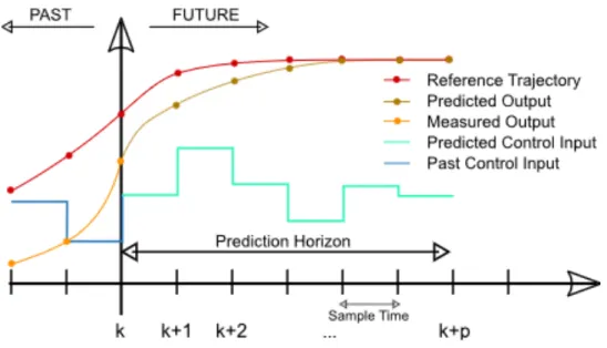
MPC can be used to control complex systems with multiple inputs/outputs. This method is particularly interesting for systems with significant delays, inverted responses or with a large number of external disturbances (Lewis et al. 2012). This corresponds to the sailboat case which has delays due to the boat inertia and a lot of external disturbances such as wind and sea state. The fundamental idea of this method is that it is built on a mathematical model of the process to control. It enables to predict the behavior of the system. It is a feedback implementation of optimal control using finite prediction horizon and online computation. At each sampling period (Figure 3), the controller:

- computes the predictions of the controlled variables for a given time horizon thanks to the internal model, it is based on measurements obtained at time t0;

- following this trajectory, determines the next control sequence to apply to the system to reach the set point. In order to ensure this, the controller seeks to minimize a cost function which differs depending on the application. Usually, this function includes quadratic errors between the reference trajectory and the predictions for the control horizon as well as the control input variations to reduce the risk of instability;

- applies the beginning of the control strategy until the next decision instant.

Figure 3: Principle of Model Predictive Control (By Martin Behrendt via Wikimedia Commons)

The main users of the predictive control are oil refineries, agri-food industries, aerospace and car industries, etc. MPC also shows a good level of performance in ship’s applications (Li et al. 2012). It enables a greater freedom to define control objectives and constraints. The hard task in the case of sailing is to adapt this control method to a much more complex behavior and to define a cost function to minimize which achieves a good level of precision and performance while taking into account the power consumption.

The cost function enables to have a scalar representation of an event. Thus, it transcribes again one or more costs associated with this event that the controller is going to minimize through this representative function.

The optimization problem 𝑃J𝑥(𝑘)K to solve is defined as: ∀𝑘 ∈ ℕ, 𝑥(𝑘) ∈ ℝP _{𝑃J𝑥(𝑘)K ∶ min}

U V 𝑉(𝑥(𝑘), 𝑢) W 𝑢 ∈ 𝑈J𝑥(𝑘)K Y (1)

𝑉(𝑥(𝑘), 𝑢) : a cost function to minimize 𝑢 : the control variable

𝑈 : a set of admissible values

So, the function 𝑉 is minimized by modifying the variable 𝑢 under the constraint 𝑢 ∈ 𝑈. This control shape could suggest a classic LQR (Linear Quadratic Regulator) problem but since it involves inequalities constraints and a finite horizon, it requires a more specific solution approach. The discretization of the system enables to define a given prediction horizon 𝑁₊.

In Tréhin et al. (2019), we proposed to define a cost function taking into account two separate criteria. Then, these criteria are minimized jointly. These are the precision and the energy used by the system:

- Criteria 1 Precision: square error minimization

𝑉₅(𝑥(𝑘), 𝑝) = \W|𝑦(𝑘 + 𝑛, 𝑝) − 𝑦_"(𝑘 + 𝑛)|W_a b 7 cd ef5 (2)

- Criteria 2 Energy: power consumption minimization over the time horizon 𝑉₇(𝑥(𝑘), 𝑝) = \ 𝑖(𝑘 + 𝑛, 𝑝). 𝑢(𝑘 + 𝑛 − 1, 𝑝)_ai

cd

ef5

(3) 𝑦 : system output

𝑦_" : system set point 𝑖 : electric current [A] 𝑢 : voltage [V]

𝑥(𝑘) : system state 𝑝 : system input 𝑄5, 𝑄7 : load factor

The variables 𝑦, 𝑖 and 𝑢 are, in practice, estimated using the mathematical model of the process. However, having set out this problem for optimization experts, we realize that this formulation can be improved. In fact, there is no precision guarantee with this criterion. It only minimizes the mean square error. Moreover, it uses a compensatory logic. The solution can have a satisfactory

weighted sum but it still can be unacceptable because too imbalanced (e.g. a very low

consumption with a bad precision result). Besides, the weighting choice can be difficult because the two criteria have different units. Their weighted sum has no physical interpretation which may lead to control decisions that may not be satisfactory.

To mitigate these weak points, the problem is reframed to use the epsilon-constraint method. This method is well known in the multi-objective optimization area (Cho et al. 2017, Ergott 2004)

• Precision constraint 𝛿(𝑘 + 𝑛) ≤ 𝜀 ∀𝑛 ∈ V1, … , 𝑁+Y 𝑦(𝑘 + 𝑛) − 𝑦"(𝑘 + 𝑛) ≤ 𝛿(𝑘 + 𝑛) (4) 𝑦_"(𝑘 + 𝑛) − 𝑦(𝑘 + 𝑛) ≤ 𝛿(𝑘 + 𝑛) • Cost function min U \ 𝑢(𝑘 + 𝑛 − 1). 𝑖(𝑘 + 𝑛) e ₍₅₎ 𝛿 : system precision [°] 𝜀 : precision constraint [°] 𝑦 : system output [°] 𝑦": system set point [°]

𝑖 : electric current [A] 𝑢 : voltage [V]

𝑁₊: prediction horizon

This epsilon-constraint definition enables to assure that the error doesn’t go over a maximum limit fixed by the designer (e.g. 10e _{degree). The system is completely controlled and the skipper is}

safe. The minimization focuses only on energy consumption. It simplifies the optimization problem so it increases the solution speed and enables to meet the specified time constraints.

However, if it is physically impossible to meet the precision constraint over the prediction horizon, the problem has no solution. It is necessary to pretest the target feasibility. The optimization problem becomes: • Target pretest If |𝑦(𝑘) − 𝑦"(𝑘)| ≤ 𝑁𝑝. ∆pqr 𝜇 = 1 (6) Else 𝜇 = 0

If the error of the system |𝑦(𝑘) − 𝑦"(𝑘)| is lower than the largest mechanically possible displacement,

the minimization problem will focus on the energy consumption to reach the set point. If the error is too large, it means that the system can’t reach the set point within the allocated time. So the main problem will focus on the precision, it will be an error minimization. This test doesn’t require powerful computing resources and ensures that the problem is resolvable.

• Precision constraint

𝛿(𝑘 + 𝑛) ≤ 𝜀 + (1 − 𝜇). 𝑀

∀𝑛 ∈ V1, … , 𝑁₊Y, 𝑀 ∈ ℝ 𝑦(𝑘 + 𝑛) − 𝑦_"(𝑘 + 𝑛) ≤ 𝛿(𝑘 + 𝑛) (7)

𝑦"(𝑘 + 𝑛) − 𝑦(𝑘 + 𝑛) ≤ 𝛿(𝑘 + 𝑛)

The error of the system must be below the precision constraint 𝜀. This constraint can be relaxed when 𝜇 = 0 thanks to 𝑀, a high value constant.

• Cost function min U x(1 − 𝜇) \ 𝛿(𝑘 + 𝑛) e + 𝜇 \ 𝑢(𝑘 + 𝑛 − 1). 𝑖(𝑘 + 𝑛) e y (8)

The minimization is still according to only one criterion thanks to the 𝜇 parameter.

The load factor concept used in the previous optimization problem enabled to tune the controller to reduce power consumption according to the battery level. This epsilon-constraint approach

formulation has an analog feature, as the precision constraint is enforced only when necessary.

4. CASE STUDY: RUDDER CONTROL

With a bottom-up approach, the first step to obtain an energy aware control is to optimize the rudder motions (Figure 1: Autopilot control loops). In fact, the performance of a sailboat is highly dependent on how the rudder is controlled in order to move with minimum disturbances (wind shift, unnecessary rudder movements, jolts, etc.). So, before going more into the details of the heading control, it appears important to optimize the rudder movements in order to go into the lowest possible power mode, while also fulfilling precision, robustness and reactivity criteria. Let’s introduce a case study of a model predictive energy aware control, the rudder control.

4.1 System model

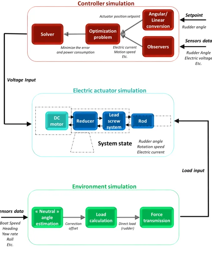
As described in the previous section, the controller is based on a mathematical description of the process. The system model consists of two subsets (Figure 4): an electric actuator model (the electric ram) and a load model (the opposing force to the ram motion). It should be noted that the controller can be designed without this second model, considering the load as a system

disturbance.

Figure 4: System model 4.1.1 Electric actuator model

The electric actuator is composed of four subsets (Figure 4):

- a DC motor (Direct Current motor) which is characterized by its inertia 𝐽_p, torque constant 𝐾}, EMF (Electromagnetic Field) constant 𝐾#, inductance 𝐿, resistance 𝑅, friction

coefficient 𝑏 “Aung (2007)”

⇒ €𝐽p𝜃̈p = −𝑏𝜃̇p+ 𝐾}𝑖 − 𝐶"#$ 𝐿𝑖 + 𝑅𝑖 = −𝐾#𝜃̇p+ 𝑢

(9)

𝜃̇_p rotation speed, 𝑖 electric current, 𝐶_"#$ resistive torque, 𝑢 voltage - a reducer modelled by its reduction ratio 𝑟, efficiency 𝑁_"

⇒ „_𝐶 𝜃̇" = 𝑟𝜃̇p

"#$…†‡ = 𝑟 𝑁_"𝐶"#$ˆ‰

(10)

𝜃_"̇ rotation speed, 𝐶_"#$ resistive torque

- a lead-screw system which is represented by the screw inertia 𝐽_Š, screw thread 𝑝 and efficiency 𝑁_Š ⇒ ‹ 𝜗 = 𝑝 2𝜋𝜃̇" 𝐶_"#$= 𝐽_Š𝜃̈_"+ 𝑝 2𝜋𝑁_Š𝐹"#$ (11)

- a rod characterized by its mass 𝑀_}

⇒ 𝐹_"#$= 𝑀_}𝛾 + 𝐹_#r- (12) 𝛾 linear acceleration, 𝐹_#r- resistive force

The accumulation of backlash in the linkage are represented by backlash on the lifting motion of the rod. It is modelled by a hysteresis which is only applied for a certain range of force and motion conditions. These conditions can boost or reduce even erase the backlash.

Moreover, the system is irreversible. That means only the motor can act on the rod of the actuator, a load force on the rod alone cannot cause a motion. This irreversible nature is represented thanks to torque’s adjustments.

4.1.2 Load model

The load model enables to estimate the mechanical power that the actuator will need to generate to move the rudder instead of experiencing this load as a disturbance. This mechanical power is directly related to the electric power consumed by the motor. By predicting the needed effort, the controller can anticipate the motion, it enables to improve the energy performance of the control significantly. This load model is composed of three sub-functions:

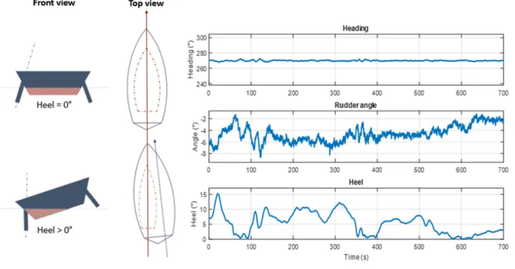
- a function of heel correction.

When the boat is heeling, as shown in the left part of Figure 5, the “neutral” angle which enables the boat to go straight ahead varies. In this figure, the data come from real navigation logs, they are not the result of simulations. They illustrate how the rudder angle varies in function of the heel in order to go straight ahead. The heel depends on the sailing conditions (sea state, wind, etc.), that is why we can observe a heel angle of 15 degrees with a rudder angle of 6 degrees. In this case, the boat is in upwind sailing on the port tack (true wind angle -42°). You can see that the boat has a constant heading with a rudder angle which oscillates around -6 degrees. It strikes a balance with a rudder angle different from 0 degree. This variation greatly affects the load calculation. So, this function enables the determination of the influence of the heel on the load calculation and to apply a correction offset.

- a function of load calculation

The function of load calculation is mainly a computation of hydrodynamic forces. The load related to the added mass is considered to be negligible. The thin foil theory is behind this computation.

𝐹_'()"* •••••••••••••⃗ = 𝐹•••⃗ + 𝐹+ •••⃗ with ‹ -𝐹+ = 1 2𝜌𝑉7𝑆𝐶+ 𝐹- = 1 2𝜌𝑉7𝑆𝐶 - (13)

Figure 5: "Neutral" angle illustration

The lift 𝐶₊ and drag 𝐶_- coefficients are defined as follows:

’

𝑘

=

𝜆 =

(14)

𝛼: angle of attack [rad]

𝑉: speed of the incident stream [m s-1_]

e: planform efficiency factor (Oswald’s coefficient)

In this model, the angle of attack 𝛼 and the speed 𝑉 of the incident stream depend on the boat speed, the rudder angle and the rotation speed of the rudder.

- a function of force transmission

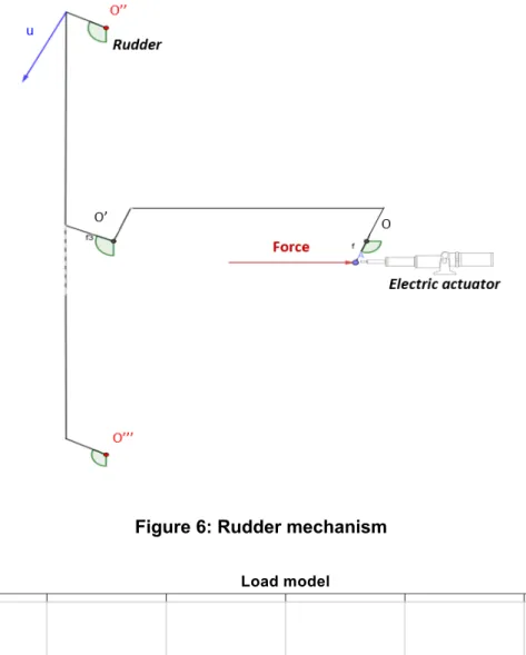
This function enables to calculate the force that acts on the actuator rod from the moment applied on the rudder’s arm and the kinematic chain between these two points. It is based on solid

mechanics. Figure 6 shows the rudder mechanism. The load is applied at points O’’ or O’’’ of the rudder and transmitted to the electric actuator via the connecting bars. The vector “Force” represents the image of this load applied at point A (the point where the actuator is fixed).

Figure 6: Rudder mechanism

This load model is validated thanks to the instrumentation of a sailboat. As shown in the graph above (Figure 7), the load simulation from the boat’s log enables a precision of +/- 20%. The actual load corresponds to a load cell measurement installed on the boat. This precision is sufficient because the load dynamic of our model corresponds to the reality. The margin of error is treated as a disturbance. This model could be improved by adding a sea state representation.

4.2 Movements representation

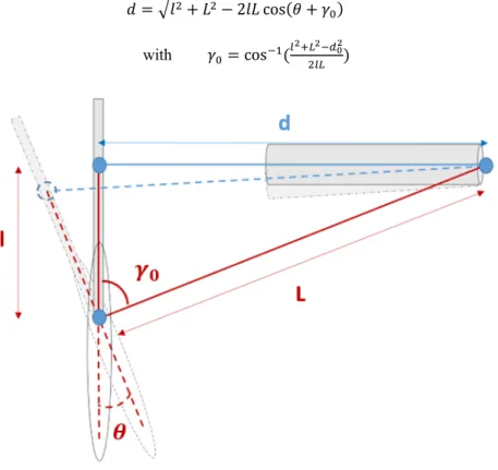
Moreover, all angular movements of the rudder are converted into linear movements of the rod (Figure 8) using the following function:

𝑑 = •𝑙7_{+ 𝐿}7_{− 2𝑙𝐿 cos(𝜃 + 𝛾}

¢) (15)

with 𝛾¢= cos£5(¤

i_–¥i_£)¦i

7¤¥ )

Figure 8: Angular/linear conversion

In fact, the control is carried out on the linear position of the rod and not on the angular position of the rudder to evade the non-linearity related to the boat installation.

So, the mathematical model for the controller design is stated. This controller is implemented into a digital system; therefore, it is necessary to discretize the model to proceed to the controller design. The selection of the discretization step must take into account the dynamic of the system to control as the selection of the controller settings.

4.3 Settings

Two tuning descriptions are detailed in this section: the prediction horizon and the control

frequency. They enable the controller to properly understand the system behavior and to not miss any important event. The mis-set of these parameters can change the dynamics of control

- The tuning of the prediction horizon

A too short horizon can lead to a system instability. To ensure stability, there is a need to respect a minimum horizon or to reduce the state vector. However, the latter solution means suboptimal control to initial requirements. On the contrary, a too long horizon can lead to an overload of the device which won’t meet the real-time conditions. To offset this problem, reduced dimensional parametrization methods can conciliate a low number of degrees of freedom and a long prediction horizon that may be necessary for stability (Lewis et al. 2012). In order to not oversize the

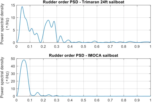
prediction horizon to ensure stability and to best adapt to every boat, frequency studies made for each sailboat category enable to guide the horizon selection. To do that, an averaged periodogram is used to estimate the power spectral density of the rudder angle. This rudder angle corresponds to the autopilot order in response to the sailboats movements (Figure 9). These studies show a correlation between the appropriate horizon length and the boat’s inertia i.e. its response to an event. For instance, an IMOCA (60ft) needs a longer prediction horizon than a “small” trimaran (24ft) to have an optimal control. In fact, the graph shows that the IMOCA has a lower range of frequency due to its greater inertia (Figure 9). The trimaran is more responsive.

Figure 9: Power spectral density for rudder angle order measurements

- The tuning of the prediction/control frequency

The right choice of prediction/control frequency enables not to miss any system event and to respond accordingly. In this case study, the events relating to the electric behavior are the most critical because they have the highest dynamics. So, this frequency must be adjusted according to the electric time constant of the motor in order to be able to track the current peaks. This time constant is defined as:

𝜏_#¤#} = 𝐿

𝑅 (16)

𝐿 motor inductance, 𝑅 motor resistance

So, the prediction/control frequency must be of the same order of magnitude as this electric time constant depends on the motor characteristics.

4.4 Control results

In order to test the control method, the performance of various controller tunings is compared in a realistic simulation environment (Figure 10). As a reminder, the objective is to design and test rudder control. The simulation environment is based on the models which are described in the first part of this case study.

The simulation inputs are derived from logs coming from real navigations. Series of simulation of navigation (5min) are run with various precision constraints to observe the impact on consumption. As a reminder, the cost function to minimize is defined as:

(1 − 𝜇) \ 𝛿(𝑘 + 𝑛) e + 𝜇 \ 𝑢(𝑘 + 𝑛 − 1). 𝑖(𝑘 + 𝑛) e ₍₁₇₎ 𝛿(k) : system precision [°] 𝑖 (𝑘) : electric current [A]

𝑢(𝑘) : voltage [V] 𝜇 : target pretest result

4.5 Tuning results

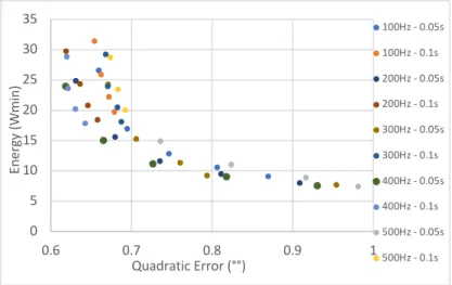
Figure 11 shows the results for various prediction horizons and frequencies. Changing the precision constraint enables to draw a Pareto Front for each tuning. In this figure, the quadratic error represents the system precision. It is used in order to penalize large errors. A prediction horizon sets to 0.05s and a frequency to 400Hz seems to give the best performance results for this sailboat. As underlined in the table, this tuning gives the best precision for about the same energy consumption.

Figure 11: Tuning results - Pareto Front

Table 12: Energy & Quadratic error

Controller Energy Quadratic Error (W.min) (°°) 100Hz – 0.05s 16.94 0.69 200Hz – 0.05s 15.56 0.68 300Hz – 0.05s 15.28 0.70 400Hz – 0.05s 15.01 0.66 500Hz – 0.05s 14.87 0.73 0 5 10 15 20 25 30 35 0.6 0.7 0.8 0.9 1 Ene rg y (W m in) Quadratic Error (°°) 100Hz - 0.05s 100Hz - 0.1s 200Hz - 0.05s 200Hz - 0.1s 300Hz - 0.05s 300Hz - 0.1s 400Hz - 0.05s 400Hz - 0.1s 500Hz - 0.05s 500Hz - 0.1s

4.6 MPC control results

The settings of the MPC controller are now fixed. We can compare its results with one control law coming from the state of the art, a Proportional Integral controller (Figure 12). The PI settings roughly correspond to those which are implemented in the standard autopilots. To obtain these data, we make 4 simulations based on navigations log:

- PI control simulation

- MPC control simulation (𝜀 = 0.1) - MPC control simulation (𝜀 = 0.3) - MPC control simulation (𝜀 = 0.7)

The (𝜀 = 0.1) simulation shows a better precision level than the PI control. However, a great precision leads to an increase of energy consumption. In fact, it moves the rudder in a more reactive way. For about the same power consumption as the PI, the (𝜀 =0.3) simulation still gives a better precision (+45%). Finally, in the (𝜀 = 0.7) simulation, the MPC control enables a better precision than the PI control with a reduced power consumption (-25%). It moves the rudder into the lowest possible power mode. These simulation settings are intended to be as realistic as possible. They use real sensor data and autopilot orders as inputs to compute the actuator responses. They are based on real actuator characteristics. Thanks to our environment and actuator simulation, the results in a real case should be close to these simulation results. Of course, only a real experiment could confirm these hypotheses which will be tested as soon as possible on a real hydrofoil sailboat.

Based on its knowledge of the system, the MPC control does more than driving the rudder from point A to point B, it uses the best way with the most appropriate speed and acceleration which reduce the energy consumption. In the case of a lack of power on board, the skipper (or the embedded system) can change online the load factor that means moving a cursor corresponding to the power he wants to allocate to the steering. The limits of the cursor are defined in advance in order to prevent a system divergence. To do so, the feasibility of the cost function minimization is checked at each bound.

All the conventional feedback design techniques are not compared with the MPC control in this study for lack of time. Some comparisons can be found in the state of the art (ex: McGookin et al. (2008)). This study approach aims to test a new control method which is not used in the sailing area but largely known in aviation, ever closer to our activities. In fact, the aviation area concerns the same actuators (rudder, flap, elevator, etc.) and the same attitude control issues as the hydrofoiling control. These results are encouraging. The MPC control puts a physical problem in mathematical form thanks to one equation. Other conventional methods would address this issue in many parts as velocity gain scheduling, integrator anti-windup or dead bands.

Figure 13: MPC/PI results

5. CONCLUSION

Our main goal is to design an energy aware autopilot for a heading and foil dynamic control. To answer this problem, in this paper, we propose a new control method which is aware of the energy consumption. This control method is based on a MPC controller which minimizes a cost function taking into account two criteria: the square error and the energy consumption. It makes a

prediction of the system behavior from an electric actuator model and a load model. This control method is then applied on a rudder control. In fact, this control loop is the first step to completely manage the autopilot system and its energy. For the same energy consumption as a PI controller, we increase by 45% the precision level or we are able to reduce the consumption by at least 25%. This controller optimizes the use of the energy onboard to steer the boat. It can be tuned online to reduce the power consumption according to the battery level. We believe that the energy

consumption results shown in this paper will be difficult to improve if we focus only on the rudder control. Maybe, they could be enhanced by working on a new cost function formulation or a new solver but It would be a lot of work for an improvement of a few percent. This solution seems to be a good compromise for the moment. However, the energy gain could be increased by working on the heading/attitude control loop represented in Figure 1. The entire autopilot system would be energy aware. We decided not to extend this study further in the hydrofoiling case because we don’t have enough background to compare our results to an existing system. In fact, this is the beginning of hydrofoil control and it is difficult to obtain data coming from a controlled hydrofoil sailboat. The next step, in the medium term, will be the coding of the method in order to enter it onto the target architecture. Then, we will have to develop a hydrofoil control law which uses this method to manage the actuators. The first step for a complete flight control is the development of a flight stabilization system which is aware of the available energy on board. It will be tested in the simulation as this optimization method before being implemented in a real hydrofoil sailboat. After these experiments, we will have enough data to extend this article to the hydrofoiling case.

6. REFERENCES

Alfi A., Shokrzadeh A., Asadi M. (2015), Reliability analysis of H-infinity control for a container ship in waypoint tracking, Applied Ocean Research, Vol. 52.

Ang K. H., Chong G., Li Y. (2005), PID control system analysis, design, and technology, IEEE Transactions on Control Systems Technology, Vol. 13, Issue 4, pp. 559-576.

Aung W. P. (2007), Analysis on Modeling and Simulink of DC Motor and its Driving System Used for Wheeled Mobile Robot, World Academy of Science, Engineering and Technology, Vol. 32, pp. 299-306.

Briere Y. (2011), Sailing robot performance: maximum speed tracking vs energy efficiency, Field Robotics - 14th _{International Conference on Climbing and Walking Robots and the Support}

Technologies for Mobile Machines, Paris, France.

Cho J-H., Wang Y., Chen I-R., Chan K.S., Swami A. (2017), A Survey on Modeling and Optimizing Multi-Objective Systems, IEEE Communications Surveys & Tutorials, Vol. 19, Issue. 3, pp. 1867-1901

Douguet R. (2013), A New Real-Time Method for Sailboat Performance Estimation based on Leeway Modeling, SNAME 21st CSYS, Annapolis, MD.

Ergott M. (2004), Multicriteria Optimization, Springer-Verlag Berlin and Heidelberg GmbH & Co. Lewis F.L. (2012), Vrabie D., Syrmos V.L., Optimal control, Hoboken, New Jersey: John Wiley & Sons, Inc.

Li Z., Sun J. (2012), Disturbance Compensating Model Predictive Control with Application to Ship Heading Control, IEEE Transactions on Control Systems Technology, Vol. 20, Issue 1, pp. 257-265.

McGookin E. W., Murray-Smith D. J., Li Y. Fossen (2000), Ship steering control system

optimisation using genetic algorithms, Control Engineering Practice, Vol. 8, Issue 4, pp. 429-443. McGookin M., Anderson D., McGookin E. (2008), Application of MPC and sliding mode control to IFAC benchmark models, UKACC International Conference on Control., Manchester, UK.

Roberts G. N. (2008), Trends in marine control systems, Annual Reviews in Control, Vol. 32, Issue 2, pp.263-269.

Shi Y., Shen C., Fang H., Li H. (2017), Advanced Control in Marine Mechatronic Systems: A survey, IEEE/ASME Transactions on Mechatronics, Vol. 22, Issue 3, pp. 1121-1131.

Tiano A., Zirilli A., Yang, C., Xiao C. (2001), A neural autopilot for sailing yachts, 9th _{MED '01}

Proceedings, pp. 27-29, Dubrovnik, Croatia.

Tomera M. (2010), Nonlinear Controller Design of a Ship Autopilot, International Journal of Applied Mathematics and Computer Science, Vol. 20, Issue 2, pp. 271-280.

Trehin M., Laurent J., Kerhascoët H., Diguet J-P. (2019), An Energy Aware Autopilot for Sailboats, SNAME 23rd _{CSYS, Annapolis, MD.}