1 Introduction
Movement and speed deeply influence our perception of the urban environment. Several methods have been proposed until now to study the visual perception of an observer in motion along a route or a path within the city.
A simple method to catch the dynamic perception of urban open spaces is to use sets of pictures, be they photographs or hand drawings, taken from different locations along a route (Bosselmann, 1998; Cullen, 1961). This method can be used to follow the variation of the morphology of urban open spaces and the evolution of visual signs, like monuments or important perspectives. Considering that the discontinuous nature of such a series of sketches rendered them unsuitable for the representation of the continuous process of transformation of vision in motion, Thiel (1961) established the basis of a sequence ^ experience notation. The graphic notation that he proposed indicates the observer's speed and direction of movement along with characteristics of open spacesöoverall dimensions, frontal or lateral definition, and so on. Lynch et al (1966) proposed to combine both approaches, sets of images and sequence ^ experience notation, in order to analyse the perception of car drivers along highways. The sequence diagrams proposed by these authors do not capture only apparent motion of the visual field, but also the apparent self motion of the observer in the three dimensional space (ups and downs, turns, and so on). Finally, using the vocabulary of film makers, Panerai et al (1999) extended this latter method and proposed to divide the route into sequences where the urban scenery was characterised by constant properties like symmetry, opening, strangle, and so on. The different sequences can
Comparing sky shape skeletons for the analysis of visual
dynamics along routes
Franc°ois Sarradin, Daniel Siret
Cerma UMR CNRS 1563, School of Architecture of Nantes, rue Massenet, BP 81931, 44319 Nantes Cedex 3, France; e-mail: francois.sarradin@cerma.archi.fr,
daniel.siret@cerma.archi.fr
Michel Couprie
Institut Gaspard-Monge, Laboratoire A2SI, ESIEE, 2 boulevard Blaise Pascal, BP 99, 93162 Nosy-Le-Grand Cedex, France; e-mail: coupriem@esiee.fr
Jacques Teller
Lema, University of Lie©ge, 1 chemin des Chevreuils B52/3, 4000 Lie©ge, Belgium; e-mail: jacques.teller@ulg.ac.be
Received 28 September 2005; in revised form 23 May 2006
Abstract. The motion of an observer in a given space produces a particular perception called motion perspective. This has been defined by Gibson as the gradual changes in the rate of displacements of contour lines in the visual field of the observer. This paper describes a new approach intended for analysing the motion perspective in order to quantify the morphology of urban open spaces along routes. It is based on spherical projections, which provide the shape of the sky boundary around the observer. The projections are studied through their skeletons, which are continuous sets of curves obtained by a progressive thinning down of the shapes around their main saliencies. The proposed method uses these skeletons to follow the variations in the shape of the sky boundary between the successive views. Measures of these variations have been developed and applied in a range of simplified theoretical examples and a real field example in order to show that they succeeded in capturing significant variations in spherical projections.
be chained into series corresponding to specific `effects' like an access on a place, an approach towards a monument, and so on.
Although all these attempts to analyse the perception of observers in motion are strongly qualitative, they have contributed to establish the importance of visual dynamics in the perception of urban environments, be they historic sites or highways. They are based on the idea of a `motion perspective' defined by Gibson (1950) as ``the gradual change in the rate of displacement of contour lines in the visual field. The change is from motion in one direction through zero to motion in the opposite direction and it has a vanishing line, at right angles to the gradient, which passes through the centre of clear vision.'' Motion perspective relates to the continuous transformation of the visual scene occurring between different static views. Initially formulated by Gibson (1950) in order to address the perception of air pilots when landing, this notion proved to be applicable to the perception of any observer in displacement. When applied to the perception of urban environments, motion perspective appears to be intrinsically dependent on the movement of the observer (speed, orientation, turns, and so on) and the nature of the environment (complexity, structure, morphology).
In this paper we propose to develop a computer method to analyse the visual dynamics of an observer in movement along a route. The analysis will be based on a series of spherical projections of the sky shape as perceived by an observer at different points on the route. The skeletons of these sky shapes will then be calculated. Skeletonisation is a mathematical technique often used in image analysis which will allow us to trace and characterise the dynamic variation of the sky shape as perceived by an observer.
The next section will present field-oriented methods and a short description of the spherical metric developed by Teller (2003). Section 3 will establish the principles of the skeletonisation, present different classes of skeletonisation algorithms which have been proposed, and describe the algorithm chosen to compute the `skeletons of the sky shapes' in our method. In section 4 we will describe some measures of skeletons which provide a quantification of variations appearing in the sky shapes. In section 5 we will discuss different tests of the measures made on simple cases and on a real case in Nantes (France).
2 Field-oriented approaches and motion perspective
Field-oriented approaches tend to assimilate the space to a set of attributes (Teller, 2003). This is a first step towards the notion of motion perspective as presented above in that such approaches allow variations in the visual field between different points of the space to be highlighted. Open spaces are indeed no longer divided into discrete surfaces and volumes, but considered as a continuous field which cannot be partitioned a priori. The use of isovists and isovist fields is one of the first and maybe the best known field-oriented method (Benedikt, 1979). On the basis of Gibson's theory, Benedikt (1979) considers all the available information around a point with respect to an envi-ronment. An isovist is a visibility area on which different measures can be applied. The surface of an isovist provides an idea of the quantity of information available around a point. The ratio between the surface and the square of the perimeter of an isovist provides its circularity. The different moments of an isovist provide its asymmetry, its orientation, and so on. Turner (2003) and Turner et al (2001) extended the notion of isovists through the use of graph theory to analyse a visibility graph. Besides the fact that it is much more effective in terms of calculation time, using graph theory allows the authors to propose new measures such as the clustering coefficient or the mean shortest path length value.
It has been argued that one of the weaknesses of isovist methods is that they do not consider 3D environments and hence ignore building heights or relief, which is not readily acceptable in dense urban environments. Fisher-Gewirtzman and Wagner (2003) proposed a method for analysing a kind of 3D isovists. The method consists in dividing the space into voxels, a unit cube associated with an information which indicates if it corresponds to a built volume or not. It is then possible to count the visible voxels from given locations. In order to avoid infinite counts, the visibility is bounded by a horizon which is a sphere around the observation point.
Ratti and Richens (2004) developed an original field-oriented method based on the application of image analysis tools on an urban plan. The method is simple and fast. Still, like the Fisher-Gewirtzman method, it is based on discrete information represent-ing the buildrepresent-ing height and it is unable to represent tunnels. Methods based on discrete representation are limited by their resolution level. A high resolution level produces good results, but leads to long computation times. Conversely, low resolution speeds up calculation times but may be inaccurate. Some methods enable the reduction of the computational complexity. For example, to improve their method, Fisher-Gewirztman et al (2005) propose to take into account only the visible cells.
Partitioning open spaces into convex areas is another field-oriented approach. It has been proposed by Peponis et al (1997). The space is partitioned such that the boundary between two adjacent partitions is due to the apparition of a visual event or a discontinuity in the visual aspect of the scene (apparition of a surface, a corner disappears, and so on). This a 2D method, but it is similar to some 3D methods developed in the field of computer graphics, such as aspect graphs (Koenderink and van Doorn, 1976), the visibility complex (Durand et al, 1996; Pocchiola and Vegter, 1996), or the visibility skeleton (Durand et al, 1997). These methods are rather heavy in terms of computation time and they do not discriminate the visual events. In other words, for these methods, a visual event generated by a small element has the same weight as a visual event generated by a large element.
Teller (2003) developed a metric of urban open spaces based on spherical projec-tions. A spherical projection is like a 3D isovist in the sense that it computes all visible information available from a point. Spherical projections of objects can be computed even if the objects are very distant, without loss of rapidity or relevant loss of memory space. Spherical views are used to analyse the urban sky shape visible from points in space. The sky shape is directly influenced by the urban configuration surrounding the observer and hence reveals some of its properties. Teller (2003) pro-posed different measures of the sky shape. The sky opening consists in computing the ratio between the surface of the sky shape and the surface of the spherical projection. It varies with the mass ratio between buildings and open space. Two other measures are based on the inertia moments of the sky shape: spreading and eccentricity. Spreading provides information about the orientation and eccentricity provides information about the asymmetry of the open space.
Even though they constituted a significant step forward in the consideration of the dynamics of perception, all these field-oriented methods fall short of capturing the gradient of change in the visual environment associated with motion perspective. They are indeed based on a mapping of the variation of given attributes throughout the open space. In the case of isovists for instance, the distance between the perception in two locations is given by the difference between measures calculated on both their isovists rather than on the actual difference between the shape of these two specific isovists. Still the latter approach is much closer to what Gibson (1950) called the motion perspective in that it could reflect the progressive deformation of the visual field of an observer in movement.
As discussed by Teller (2003), the sky shape, namely the spherical projection of the sky, is a good three-dimensional descriptor of the urban morphology as perceived from one location. An analysis of the continuous deformation of the sky shape along a path hence constitutes a promising way to characterise the perception of observers in movement along a route in the city. Analysing this deformation will be achieved by measuring the distance between the skeletons of these sky shapes. Skeletonisation is a mathematical technique that allows the transformation of a continuous shape into a graph structure retaining its geometrical characteristics and highlighting its main saliencies.
Extensively used in map generalisation and road extraction applications (Leymarie et al, 2005), skeletonisation has not been widely applied in urban open space analysis so far. Carvalho and Batty (2005) highlighted that skeletonisation is not readily applica-ble for extracting axial lines from binary images and developed an alternative method based on the analysis of maximal straight lines. This further confirmed the significance of isovist maximal distance already highlighted by Batty (2001). In a quite different approach this technique will be used in this paper for measuring the similarity between different shapes once `synthesised' through their skeleton.
3 Skeletonisation methods
Originally proposed in the 1960s by Blum (1967), skeletonisation has progressively found applications in a number of research fields. It is now a popular image analysis technique which is used in medical imagery, mineralogy, shape recognition, and so on. A variety of computer algorithms have been proposed for different casesöfor contin-uous or discrete spaces, for polygonal or curve boundaries, for shapes with or without holes, and so on. This section presents definitions and properties of skeletonisation and the algorithm we have used in order to compute sky shape skeletons.
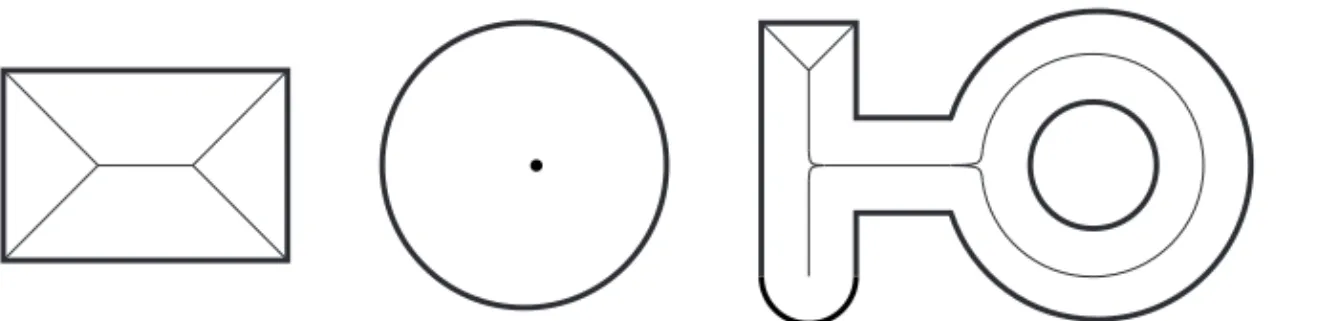
In simple terms, skeletonisation, consists of thinning down a shape until a set of centred lines is obtained (figure 1). The set of lines is called a skeleton or medial axis. The formal definition of the skeleton is based on the notion of a maximal ball. A matrix ball B is a ball (or a circle) inscribed in a shape S, for which there does not exist any other inscribed ball B0 in S, such that B0 contains B. A skeleton M(S ) of a shape S is
defined as the set of centres of maximal balls in S. The weighted skeleton or medial axis transform MT(S ) is defined as the set of pairs composed by the centres of the maximal
inscribed balls and their radii.
Skeletons are characterised by quite remarkable properties that make them very suitable for comparing different shapes. First, they are theoretically invariant under geometrical transformations. Each weighted skeleton is unique and the skeletonisation is a reversible transformation, in the sense that a shape can be entirely rebuilt from its weighted skeleton. A weighted skeleton provides a hierarchical description of the shape: the skeletal points which are far from the boundary describe global aspects of the shape, while skeletal points near the boundary often relate to minor contour alterations. Finally, skeletons are homotopic: each skeleton has the same topological properties of its original shape.
A variety of techniques have been proposed to build a skeleton from any given shape. The skeletonisation methods found in the scientific literature can be divided into four main classes:
1. Topological thinningöthese skeletonisation methods are based on discrete images and consist in iteratively removing some contour points of the shape while preserving its topological characteristics. Additional constraints such as curve extremity detection and preservation are added to obtain a result which approximates the medial axis of the shape.
2. Extraction of the distance mapöthe distance map of a shape S consists in associat-ing to every point of S its distance to the closest point of the boundary of S. In the continuous framework, the local maxima (in a certain sense) of the distance map are exactly the points of the medial axis of S. This property has been used by several authors to extract approximate medial axes based on the Euclidean distance, or exact medial axes based on discrete distances.
3. Fire front simulationöthese methods are based on the evolution of the `fire front' in time. Every formation of `shock' in the front is added in the skeleton.
4. Analytic computationöthe research of the skeleton is assimilated to a geometrical problem. The methods of this kind use, for example, the polygonisation of the boundary or its Voronoi diagram.
We have tested four different methods for calculating the skeleton of sky shapes: one developed by Thiel (1994) which is based on the extraction of the distance map, another one developed by Ogniewicz (1993) which uses the Voronoi diagram of the shape boundary, a method developed by Siddiqi et al (2002) which is based on the fire front simulation, and a last one developed by Couprie and Zrour (2005) based on the extraction of the distance map.
Sky shapes were calculated for a series of spherical projections equally distributed along a route (figure 2). In our case, the distance between successive views was arbi-trarily fixed at 1 m, but this distance should obviously vary with the speed of the observer. Sky shapes are captured as raster files for each spherical projection. The four skeletonisation methods were hence applied to raster-based descriptions of the sky shape. This was an important constraint because some methods, like analytic computation are known to work better with vector-based descriptions of shapes.
The methods developed by Thiel (1994) and by Ogniewicz (1993) proved to be inaccurate because both are based on an approximation of the Euclidean distance or on a heuristic to extract the skeleton. The method developed by Siddiqi et al is very accurate, but the only implementation we had access to was very slow and was not successful for images with more than two shapes or with holes. The method developed by Couprie and Zrour (2005) is the only one which proved to be both accurate and fast. The method of Couprie and Zrour (2005) can be seen as an hybrid between class 1 (topological thinning) and class 2 (extraction from the distance map) algorithms. First, an exact Euclidean distance map D(S ) is computed from the shape S. An exact discrete Euclidean medial axis is then extracted from D(S ). This discrete medial axis is, in general, not homotopic to S and may contain too many points. Unessential points are filtered out on the basis of two geometrical criteria. The first one is the radius of the maximal ball corresponding to the point p which is considered. The second one is an angular measure, called bisector angle, defined as the maximal unsigned angle formed by the point p (as the vertex) and any two points of the contour of S which are at minimal distance from p. A filtered medial axis is obtained from the discrete medial axis by removing a point which have a small bisector angle or a small associated radius. In order to get a result which is homotopic to S, a homotopic thinning algorithm is applied on S with the constraint of preserving the points of the filtered medial axis.
4 Analysis of sky shape skeletons
As pointed out by many authors, a skeleton is a very powerful shape descriptor. It reveals a number of characteristics of the shape which may not be readily legible from its borderlines. However, available methods to interpret these skeletons are limited to the reconstruction of the shape from a skeleton (Tek and Kimia, 1999) or to shape recog-nition (Klein et al, 2000; Ogniewicz, 1993). None of the methods we have referred to describes particular attributes of skeletons. It seems that, until now, scientific research has been concentrated on methods for extracting skeletons rather than on their interpretation. This section presents two measures which allow the study of the configuration of sky shape skeletons or the comparison of series of sky shape skeletons. These measures are the greatest maximal disk and the modified Hausdorff distance, respectively. The combination of these two measures will provide a way to trace visual events appearing along routes in urban open spaces.
4.1 Greatest maximal disk
The greatest maximal disc (GMD) of a shape S is the set of all points in MT(S ) that
are most distant from the boundary of S (Sarradin et al, 2003). In the GMD set, we are interested in only one point: the one that is as close as possible to the part of the horizon in front of the observer. This point, which is a point of the MT(S ), is denoted
VGMD.
Two attributes can be extracted from the VGMD: its size and relative location. The
size of the VGMD is the radius associated to this skeletal point, that is the radius of
the largest disk or circle that can be drawn from this point as the centre and still be inscribed in the shape. It may vary between 0, if there is no open space, and the radius of the projection disk, if there is no built volume above the observer's horizon. The relative location varies between ÿ100% and 100%. It will tend towards the radius of the projection disk when the observer is progressing towards or away from a distant opening in a very closed environment. It is equal to 0% when the maximal circle circumscribed by the sky shape is centred in the projection disköin the centre of a place, for instance.
These measures have been applied to two simple configurations, cross and tee (figure 3). Proposed skeleton measures will first be applied to the cross configuration and then to both configurations.
As illustrated in figure 4, the VGMD radius is closely related to the sky opening
defined by Teller (2003) as both measures will vary with the overall size of the sky shape. By contrast the VGMDrelative location conveys a sense of orientation which was
not present in spherical measures proposed until now. For the same point, it will indeed vary according to the direction of movement. In the case of the cross environ-ment, differences between points at 30 m and 70 m are explained by the fact that in the first case the observer is moving towards an opening while in the latter case he or she is moving away from it. The sky opening and VGMD radius are identical in these two
points. VGMD relative location hence provides a measure of movement based on the
relative distance of the dominant opening in the visual field of the observer. It is not yet a genuine measure of motion perspective, as it does not compare sky shapes per se, but it provides a baseline for identifying key events in the open space variation.
50 m 50 m 50 m 50 m 50 m 50 m 10 m 10 m 50 m (a) (b) 10 m 10 m
Figure 3. (a) Cross and (b) tee configurations.
Percentage of maximum of measure 80 60 40 20 0 ÿ20 ÿ40 ÿ60 ÿ80
Projection radius for the VGMDsize
Projection diameter for the VGMD relative location
Projection area for sky opening
0 10 20 30 40 50 60 70 80 90 100
Distance (m)
Figure 4. Variations in the VGMD measures and in the sky opening in the cross configuration.
4.2 Hausdorff distance
The Hausdorff distance (DH) is regularly used in image analysis. It is considered as a
natural similarity measure between shapes (Rucklidge, 1996). The Hausdorff distance is the ``maximum distance of a set to the nearest point in the other set'' (Rote, 1991).
Let S and T be two point sets. The Hausdorff distance is defined by
DH S, T max f S, T , f T, S , (1)
where f is the relative Hausdorff distance. It is defined by f S, T max
p 2 S d p, T . (2)
The Euclidean distance (dE) is the distance usually adopted for calculating the
distance d. DH(S, T ) is null if and only if S T, and it grows as differences appear
between S and T.
It has been argued that the Hausdorff distance is not really adapted to the comparison of shape from skeletons (Choi and Seidel, 2001). Indeed, skeletonisation is a transformation which is quite sensitive to perturbations of the shape. Even if the difference between two shapes is relatively small (the shapes are very similar to each other), the extremity branches of their respective skeletons can be quite different. In such a case the Hausdorff distance between skeletons would not reflect the similarity between original shapes.
In order to solve this problem Choi and Seidel (2001) proposed replacing the Euclidean distance by the hyperbolic distance (dh) in the equation for the Hausdorff
distance (figure 5). Let P1( p1, r1) and P2( p2, r2) be two skeletal points of a shape S
[ie P1, P2 in MT(S )]. The hyperbolic distance is defined by
dh P1, P2 max0, dE p1, p2 ÿ r1 ÿ r2 . (3)
Choi and Seidel (2001) demonstrated that the hyperbolic distance was less sensitive to perturbations appearing in the skeletons and that it was more accurate for the com-parison of shapes from their skeletons. Introducing the radii, r1 and r2, of the skeleton
points within the distance equation is actually a way to take into consideration the relative importance of these points. Points located at the periphery of the shape are most influenced by small perturbations of the shape. They are at the extremity of the skeleton and they will have a small radius. Contrary to this, points located near the centre of the shape are not much influenced by small perturbations. These top nodes of the skeleton will have a greater radius. If the maximal Euclidian distance between two skeletal points is observed between a node at the centre and another one at the periphery, it should consequentially be reduced to acknowledge the respective significance of these two points. The hyperbolic Hausdorff distance has been tested for the comparison of pairs of sky shape skeletons all along a path (Sarradin et al, 2003). These tests still highlighted a
p1 d p1 p1 d d r1 r2 r2 r1 r2 r1 p2 p2 p2 dh(P1jP2) dh(P2jP1) dh(P1jP2) dh(P2jP1) dh(P2jP1)
major drawback of this measure in our research as it is not fitted to discriminate quite different environments. This can be explained by comparing the two configurations, cross and tee, presented in figure 3. In each configuration, the virtual observer's route starts from the left side and ends at the right side. The variation of the Hausdorff distance is exactly the same in both configurations.
This lack of sensibility is explained by the fact that the hyperbolic Hausdorff distance f is based on the maximum distance between the two compared sets. In the case of the tee and cross configurations this maximal distance is equivalent as both branches of the cross skeleton are similar to the branch appearing in the cross. The discrimination between these two shapes would require the effects of both branches in the cross configuration to be summed up somehow. It would require the maximum function in the relative Hausdorff distance to be replaced by another function which would be able to take all the variations between the sets into account. This is what we proposed in the modified Hausdorff distance.
4.3 Modified Hausdorff distance
The modified Hausdorff distance DMHwas developed by Dubuisson and Jain (1994). The
authors consider it as the best distance for object matching, derived from the Hausdorff distance. DMH is defined by
DMH S, T maxg S, T , g T, S , (4)
where g S, T ) is the relative modified Hausdorff distance. It is defined by g S, T jS j1 X
p 2 S
d p, T . (5)
The modified Hausdorff distance is based on the average of differences between the two sets of points being compared. This allows us to take into account all variations appearing between one set and another in a single measure. DMH may vary from 0,
if there is no change, to the projection diameter. Naturally, in g (S, T ) [equation (5)], the distance d ( p, T ) must be replaced by the hyperbolic distance [equation (3)], in order to adapt DMH to the comparison of shapes from their skeletons.
Figure 6 highlights that the variation of DMH is more important in the cross
than in the tee environment. The two peaks of figure 6 indicate the appearance and disappearance of the branch(es) from the observer's visual field and the two points where the modification induced by these two effects is the strongest.
Difference (%) 3.5 3.0 2.5 2.0 1.5 1.0 0.5 0.0 Cross DMH Tee DMH 0 10 20 30 40 50 60 70 80 90 100 Image number
Figure 6. Difference between the cross environment and the tee environment according to the modified Hausdorff distance DMH.
We have presented three measures in this section to analyse the urban open spaces along a route from skeletons of the sky shapes. Those based on the VGMD (its size and
its location) analyse the largest opening appearing around the observer at each of its steps. The third one, DMH, analyses each pair of successive skeletons. This measure
highlights successively the variations in the morphology of the urban open spaces along the route.
5 Application of sky shape skeleton measures
With a series of spherical projections obtained along a route in urban open spaces and with the help of skeletonisation, it is possible to follow the variations of the sky shape. This section presents the application of our method on simple theoretical cases and on a real case in Nantes.
The implementation of our method has been divided into three parts: the computation of the spherical projections, the skeletonisation, and the analysis of skeletons. For the spherical projections, we have implemented the algorithm used by Teller and Azar (2001) in Java. A stereographical projection has been used to flatten the spherical views on a plane as this projection best respects sky shapes (Teller, 2003). The skeletonisation has been implemented in C language. The implementation is fast enough and does not need too much memory space. On a computer with a 2.6 GHz processor, for one hundred projections with a diameter of 500 pixels, the process is not longer than a minute, even with high-definition urban environments (more than 20 000 three-dimensional faces).
5.1 Simple theoretical cases
Our method was tested on several simple cases, like a simple straight street, a street with a narrowing, different crossroads with three or four branches. In this paper, all measures are normalised according to the potential maximum of the measure. Distances are expressed in metres.
The first cases consist of a comparison between a simple corridor configuration with what we have called battlement configuration. Both configurations are composed of two walls 100 m long and 10 m high. In the second case, battlements were added at the top of the walls (figure 7). The observer's route starts on the left side and ends on the right side. It is located in the middle of the street.
Figure 8 presents the difference between the VGMD size and the sky opening
meas-ures in the simple corridor and the battlement environments. In the simple corridor configuration, the extremities of the street affect the sky opening measure all along the route, as it is a measure that considers the whole sky image in each projection. This is not the case for the VGMD size measure, which is not affected by the extremities of the
street between 12 m and 88 m. In contrast, the VGMD size measure is influenced by
the battlement configuration, which is not the case for the sky opening as the surface of the sky shape almost does not vary along the route once entered in its central area. This comparison clearly highlights that the VGMD size is much more sensitive to local
events than the sky opening, which better reflects the global configuration of the open space.
5 m 5 m
10 m 10 m
Figure 9 compares the evolution of the modified hyperbolic Hausdorff distance in both environments. In the simple corridor configuration, the curve is characterised by an almost rectilinear curve close to 0% between the 30 m and 80 m distances. There is no motion perspective in all this area, that is to say that there is no apparent variation of the observer visual field between these two points. By contrast, the curve maintains well above 0.5% in the battlement configuration. There is indeed a constant transfor-mation from one spherical projection to the next one in this case. The battlements guarantee the perception of movement all along the path. This effect would not be easily detectable through a 2D analysis. Neither is it revealed by the sky opening variation. Percentage of maximum of measure 60 50 40 30 20 10 0 10 20 30 40 50 60 70 80 90 100 Distance (m) Corridor VGMD size Battlement VGMD size Sky opening
Battlement sky opening
Figure 8. Evolution of the VGMD size and the sky opening in the simple corridor versus battlement
configuration. The ordinate values are computed according to the theoretical maximum of each measure. For a discussion of VGMD.
Battlement DMH Corridor DMH Difference (%) 3.0 2.0 1.0 0.0 0 10 20 30 40 50 60 70 80 90 100 Image number
Figure 9. Evolution of the modified Hausdorff distance DMH in the simple corridor versus
To go further in the detection of artefacts which could not be easily noticed by 2D methods, we have studied the evolution of these measures along a route through an arch configuration (figure 10).
The evolution of our measures is presented in figures 11 and 12. The crossing under the arch appears clearly at 60 m. VGMD and sky opening measures are affected a bit
more than 10 m before and after the arch. Apart from the amplitude, there are no important differences between the VGMD size and the sky opening variation in this case.
The entrance and exit under the arch are clearly indicated by two peaks of the modified Hausdorff distance. Furthermore, DMH, unlike VGMD measures, varies all
along the route and reaches a minimal value at 20 m and 90 m, namely where the configuration is most similar to a simple corridor configuration. It confirms that this measure is much more sensitive to motion than VGMD ones.
Figure 13 presents the influence of speed on DMH in the cross configuration
[figure 3(a)]. For the three curves, we have used different sampling: an image every 2 m for speed 2, an image every metre for speed 1, and an image every 0.5 m for speed 0.5.
3 m 7 m 10 m 10 m 10 m 20 m 10 m 10 m 10 m 50 m 20 m 50 m 3 m 4 m 3 m
Figure 10. Description of a route through an arch configuration.
Percentage 70 60 50 40 30 20 10 0 ÿ10 ÿ20 ÿ30 VGMD size VGMD position Sky opening 0 10 20 30 40 50 60 70 80 90 100 Distance (m)
Figure 11. The evolution of the VGMD measures and the sky opening in the arch configuration.
Assuming that images are separated by a same time delay, each sampling represents a different speed. Figure 13 reveals that the higher the speed, the higher the difference between successive images. Furthermore, speed tends to lessen variation details or secondary events that appear in low speed curves. Speed has no effect on the other measures (VGMD and sky opening).
Our measures have been tested in other simple configurations. These tests served to evaluate the sensitivity and margin of error of our algorithms. They also highlighted the capacity of the proposed measures to detect visual events and assess their magnitude. Still, such simple configurations do not allow us to test the practicability of this tool in real world situations where spatial configurations are characterised by a multiplicity of events and effects.
5.2 Analysis of a real case in Nantes
We tested our method on a real case in Nantes (France). The route has been done in a 3D model of the centre of the city. This is a large model with about 87 000 3D faces.
Difference (%) 4.0 3.5 3.0 2.5 2.0 1.5 1.0 0.5 0.0 DMH 0 10 20 30 40 50 60 70 80 90 100 Image number
Figure 12. The evolution of the modified Hausdorff distance DMH in the arch configuration.
Difference (%) Speed 2 Speed 1 Speed 0.5 7 6 5 4 3 2 1 0 0 10 20 30 40 50 60 70 80 90 100 Path advance (%)
Figure 13. Influence of the observer speed on the modified Hausdorff distance DMH in the cross
The route is about 500 m long between Place du Pilori and Place Royale and it crosses a large avenue, called Cours des Cinquante Otages. A projection has been calculated every metre. The observer turns six times at points A (41 m), B (138 m), C (143 m), D (268 m), E (312 m), and F (435 m)öthese points will be referred to as `turns' in the rest of the paper.
The graph of the variation of VGMD and sky opening values (figure 15)
discrimi-nates five main openings, characterised by peaks labelled from 1 to 5 on figures 14 and 15. The most important openings are Place du Pilori (peak 1), Cours des Cinquante Otages (peak 4), and Place Royale (peak 5). Peaks 2 and 3 are due to a succession of small openings, namely lateral streets crossing the route of the observer. Narrow streets and corridor-like configurations are characterised by a constant sky opening value.
The variation of the relative location of VGMD (figure 15) emphasises what has been
noticed through the analysis of the variation of the sky opening and the size of the VGMD. Six main zones, labelled from 10 to 60, can be identified from the graph. The
route is characterised by four main visual events (20, 30, 40, and 50) related to openings
along the route. The appearance and disappearance of each of these events are bounded by a sharp increase of the VGMD location followed by a gradual decline and
another increase once past the area of influence of this event. The curves pass through zero at the centre of the opening. It is positive when the event is located in front of the observer and negative when on its back but still influencing significantly the sky shape. The magnitude of the fifth event (50) is much larger than the other ones as it relates to
the very large opening of the Cours des Cinquante Otages. The first (10) and sixth (60)
visual events are only partial ones. In the first case the event corresponds to the exit from the first place (negative VGMD location) and in the second to the arrival in the last
one (positive VGMD location).
Nine main peaks, labelled from 1 to 9, appear in the graph of the modified Hausdorff distance (figure 16). The first three peaks (1, 2, and 3) correspond to locations where
10 20 30 40 50 60
1 2 3 4 5
0 50 100 150 200 250 300 350 400 450 500 distance (m)
Figure 14. A part of the model of the centre of Nantes and the route followed by the observer. The bar at the top of the figure represents the length of the path, and is nonlinear as the path is not straight.
the observer turns (turns A, B, and C). These turns were modelled as instant modifications of the observer's direction of view, concomitant with the modification of his or her own direction of movement. When the turn is important, as in the first three points, they provoke sharp contrasts in the orientation of the sky shape. A more gradual change of the direction of view would obviously smooth such peaks. The next peaks (4 and 5) mark the entrance and exit from the Cours des Cinquante Otages combined with a very
Percentage 60 50 40 30 20 10 0 ÿ10 ÿ20 ÿ30 1 2 3 4 5 10 20 30 40 50 60 0 50 100 150 200 250 300 350 400 450 500 Distance (m) VGMD size VGMD position Sky opening
Figure 15. The evolution of the size of the VGMD measures and of the sky opening along the route
in Nantes. For a discussion of VGMD see text.
Difference (%) 4.0 3.5 3.0 2.5 2.0 1.5 1.0 0.5 0.0 1 2 3 4 5 6 7 8 9 0 50 100 150 200 250 300 350 400 450 500 10 20 30 40 50 60 70 Distance (m) DMH
little change in the direction of view. Peak 6 is related to the disappearance of an opening at the right of the observer. It has to be noted that the appearance of this opening was somehow `shadowed' by the disappearance of the Cours des Cinquante Otages. Peaks 7 and 8 mark the appearance and disappearance of a street crossing the observer's route. Finally, peak 9 marks the entrance within the Place Royale, combined with the effect of a small turn.
We can further distinguish seven sequences characterised by specific profiles in the graph of DMH. They are labelled from 10 to 70 on figure 16. The first sequence
corre-sponds to the exit from the first triangular place. The sequence is characterised by a gradual decrease of DH from one view to another. Once the street has been entered,
after turn A, DH is maintained at a low and constant value very similar to a
corridor-like configuration mentioned here above (area 20). The observer then enters a sequence
characterised by various visual events and DMH values higher than 0.5% (area 30)
followed by another corridor-like sequence (area 40). The crossing of the Cours des
Cinquante Otages (area 50) is characterised by quite high D
MH values which can be
explained by the visibility of distance objects like the church or tall buildings along all this part of the route. The observer then enters a very narrow and regular street (area 60), where the sensation of movement is very weak, preceding the entrance within
the Place Royale (area 70), where once again D
MH values are affected by the visibility of
distant signs.
A combined interpretation of figures 15 and 16 would lead to combine area 10 and
20 within one single sequence bordered by two open spaces and characterised by a
gradual decrease and increase of the observer's stimulation. On the other hand the low stimulation characterising sequences 40 and 60 contribute to maximise the effect of the
Cours des Cinquante Otages (50), which undoubtedly constitutes the dominant feature
of this route, both in terms of opening and stimulation. Sequence 30 appears as a
transition between the first part (10and 20) and second part (40, 50, and 60) of the route.
6 Conclusion
We have described a new method to analyse the visual dynamics along routes. The method is based on the computation of a series of spherical projections of sky shapes along a route, and skeletonisation is used to study the continuous deformation of the observer's visual field. Different measures have been proposed in order to analyse these variations: two measures based on the VGMD(its size and its relative location) and one
measure using the modified Hausdorff distance. The method has been tested on different simple examples and a real application in the city of Nantes.
Our method is an extension of the method of spherical metrics introduced by Teller (2003); spherical metrics are similar to three-dimensional isovists. Most interestingly, spherical projects transform an infinite unbounded 3D scene into a finite bounded 2D view, respecting given relations between objects. The main advance of our skeleton-based method when compared with existing spherical metrics is to allow comparisons of sky shapes, and hence to provide a way to describe the motion-based perspective once introduced by Gibson (1950).
Simple tests highlighted that the proposed method detects main events character-ising a route and, most importantly, determines their location and amplitude. The application of sky shape skeleton measures to the analysis of a route in Nantes reveals a complex structure web of open spaces and visual events. It emphasises the 3D nature of the observer's experience and confirms the interest of the DMH as a motion-based
perspective indicator. The set of sequences derived from this graph is much richer than that based on the combination of sky opening and VGMD measures, which neglect a
objects, and the like. However, DMH graphs would probably be difficult to interpret
without the prior knowledge of the baseline structure that appears in other graphs. This surely advocates for the combination of these different measures through a typology of visual effects.
Further development can be made to get methods to sequence or qualify urban routes according to a predefined typology of indicators. Other improvements can be done by integrating the method into a 3D-GIS tool. Finally, the method could be further tested in different cases such as cities outside Europe, city outskirts, in wide open landscapes, which would not be `propelling' the observer along a route as was the case in the path through Nantes discussed in this paper. Low-density environments are indeed usually characterised by a large sky opening and reduced variations in the sky shape between one point and another. Analysing the flow of visual information in such environments may hence require a shift of the focus on proposed measures from the sky shape to the built fabric itself in order to capture the variation of view length spherical distribution (Teller, 2003).
References
Batty M, 2001, ``Exploring isovist fields: space and shape in architectural and urban morphology'' Environment and Planning B: Planning and Design 28 123 ^ 150
Benedikt M L, 1979, ``To take hold of space: isovists and isovist fields'' Environment and Planning B 6 47 ^ 65
Blum H, 1967,``A transformation for extracting new descriptors of shape'', in Proceedings of Models for the Perception of Speech and Visual Form (MIT Press, Cambridge, MA) pp 362 ^ 380 Bosselmann P, 1998 Representation of Places: Reality and Realism in City Design (University of
California Press, Berkeley, CA)
Carvalho R, Batty M, 2005, ``Encoding geometric information in road networks extracted from binary images'' Environment and Planning B: Planning and Design 32 pp 179 ^ 190
Choi S W, Seidel H P, 2001, ``Hyperbolic Hausdorff distance for medial axis transform'' Graphical Models 63 369 ^ 384
Couprie M, Zrour R, 2005, ``Discrete bisector function and Euclidean skeleton'', in Proceedings of Discrete Geometry for Computer Imagery (Springer, Berlin) 216 ^ 227
Cullen G, 1961 The Concise Townscape (Architectural Press, London)
Dubuisson M P, Jain A K, 1994, ``A modified Hausdorff distance for object matching'', in Proceedings of the 12th International Conference on Pattern Recognition pp 566 ^ 568
Durand F, Drettakis G, Puech C, 1996,``The 3D visibility complex: a new approach to the problems of accurate visibility'', in Proceedings of the 7th EurographicsWorkshop on Rendering (Rendering Techniques '96) pp 245 ^ 257
Durand F, Drettakis G, Puech C, 1997, ``The visibility skeleton: a powerful and efficient multi-purpose global visibility tool'', in Proceedings of SIGGRAPH'97 pp 89 ^ 100
Fisher-Gewirtzman D, Wagner I, 2003, ``A 3D visual method for comparative evaluation of dense built-up environments'' Environment and Planning B: Planning and Design 30 575 ^ 587 Fisher-Gewirtzman D, Shach D, Wagner I A, Burt M, 2005, ``View-oriented three-dimensional
visual analysis models for the urban environment'' Urban Design International 10 23 ^ 37 Gibson J J, 1950 The Perception of the Visual World (Houghton Mifflin, Boston, MA) Klein P, Tirthapura S, Sharvit D, Kimia B, 2000, ``A tree-edit distance for comparing simple,
closed shapes'', in Proceedings of the Symposium on Discrete Algorithm (SODA '00) pp 696 ^ 704 Koenderink J J, van Doorn A J, 1976, ``The singularities of the visual mapping'' BioCyber 24
51 ^ 59
Leymarie F, Boichis N, Airault S, Jamet O, 2005, ``Semi-automatic road tracking'' Proceedings of the Remote Sensing for Geography, Geology, Land Planning and Cultural Heritage Conference SPIE 2960, pp 84 ^ 95
Lynch K, Appleyard D, Myer J R, 1966 The View from the Road (MIT Press, Cambridge, MA) Ogniewicz R L, 1993 Discrete Voronoi Skeletons PhD thesis, ETH-Zurick, Zurich
Panerai P, Depuale J C, Demorgon M, 1999 Analyse Urbaine (Editions Parenthe©ses, Marseilles) Peponis J, Wineman J, Raschid M, Kim S H, Bafna S, 1997, ``On the description of shape and
spatial configuration inside buildings: convex partitions and their local properties'' Environment and Planning B: Planning and Design 24 761 ^ 781
Pocchiola M,Vegter G, 1996, ``The visibility complex'' International Journal on Computational Geometry and Applications 6 279 ^ 308
Ratti C, Richens P, 2004, ``Raster analysis of urban form'' Environment and Planning B: Planning and Design 31 297 ^ 309
Rote G, 1991, ``Computing the minimum Hausdorff distance between two point sets on a line under translation'' Information Processing Letters 38 123 ^ 127
Rucklidge W, 1996 Efficient Visual Recognition Using the Hausdorff Distance (Springer, Berlin) Sarradin F, Siret D, Teller J, 2003, ``Visual urban space assessment from sky shape analysis'', in
Proceedings of EnviroInfo 2003 pp 231 ^ 238
Siddiqi K, Bouix S, Tannebaum A, Zucker S W, 2002, ``Hamilton ^ Jacobi skeletons'' International Journal of Computer Vision 48 215 ^ 231
Tek H, Kimia B B, 1999, ``Perceptual organization via symmetry map and symmetry transforms'', in Proceedings of the IEEE Conference on Computer Vision (ICCV '99) 2 2470 ^ 2477
Teller J, 2003, ``A spherical metric for the field-oriented analysis of complex urban open spaces'' Environment and Planning B: Planning and Design 30 339 ^ 356
Teller J, Azar S, 2001, ``Townscope II: a computer system to support solar access decision making'' Solar Energy Journal 70 187 ^ 200
Thiel E, 1994 Les Distances de Chanfrein en Analyse d'Images: Fondements et Applications PhD thesis, Universite¨ Joseph Fourier (Grenoble I), France
Thiel P, 1961, ``A sequence experience notation for architectural and urban spaces'' The Town Planning Review 32 33 ^ 52
Turner A, 2003, ``Analysing the visual dynamics of spatial morphology'' Environment and Planning B: Planning and Design 30 657 ^ 676
Turner A, Doxa M, O'Sullivan D, Penn A, 2001, ``From isovists to visibility graphs: a methodology for the analysis of architectural space'' Environment and Planning B: Planning and Design 28 103 ^ 121


![Figure 13 presents the influence of speed on D MH in the cross configuration [figure 3(a)]](https://thumb-eu.123doks.com/thumbv2/123doknet/6274899.163862/12.804.49.751.121.412/figure-presents-influence-speed-mh-cross-configuration-figure.webp)


