Impact of topology-related attributes from Local Binary Patterns on texture classification

HAL Id: hal-01118009

https://hal.archives-ouvertes.fr/hal-01118009

Submitted on 18 Feb 2015

HAL is a multi-disciplinary open access

archive for the deposit and dissemination of

sci-entific research documents, whether they are

pub-lished or not. The documents may come from

teaching and research institutions in France or

abroad, or from public or private research centers.

L’archive ouverte pluridisciplinaire HAL, est

destinée au dépôt et à la diffusion de documents

scientifiques de niveau recherche, publiés ou non,

émanant des établissements d’enseignement et de

recherche français ou étrangers, des laboratoires

publics ou privés.

Impact of topology-related attributes from Local Binary

Patterns on texture classification

Thanh Phuong Nguyen, Antoine Manzanera, Walter G. Kropatsch

To cite this version:

Thanh Phuong Nguyen, Antoine Manzanera, Walter G. Kropatsch. Impact of topology-related

at-tributes from Local Binary Patterns on texture classification. ECCV Workshop on Computer Vision

with Local Binary Patterns Variants, Sep 2014, Zürich, Switzerland. �hal-01118009�

Impact of topology-related attributes from Local

Binary Patterns on texture classification

Thanh Phuong Nguyen, Antoine Manzanera, and Walter G. Kropatsch

ENSTA-ParisTech, 828 bd des Mar´echaux, 91762 Palaiseau CEDEX, France

PRIP group, Favoritenstrae 9/186-3, A-1040 Wien, Austria {thanh − phuong.nguyen, antoine.manzanera}@ensta −

paristech.f r, krw@prip.tuwien.ac.at

Abstract. A general texture description model is proposed, using topol-ogy related attributes calculated from Local Binary Patterns (LBP). The proposed framework extends and generalises existing LBP-based

descrip-tors like LBP-rotation invariant uniform patterns (LBPriu2_{), and Local}

Binary Count (LBC). Like them, it allows contrast and rotation invari-ant image description using more compact descriptors than classic LBP. However, its expressiveness, and then its discrimination capability, is higher, since it includes additional information, including the number of connected components. The impact of the different attributes on texture classification performance is assessed through a systematic comparative evaluation, performed on three texture datasets. The results validate the interest of the proposed approach, by showing that some combinations of attributes outperform state-of-the-art LBP-based texture descriptors.

Keywords: local binary pattern, local descriptor, texture classification

1

Introduction

Texture recognition is a very active research topic in computer vision and pattern recognition. One of the most popular approaches for texture classification is based on feature distribution using Local Binary Pattern (LBP), introduced in [1]. Since the generalised work of Ojala et al. [2], LBP is widely considered as an efficient descriptor for capturing local properties of images. The decisive advantages of LBPs are their low computational cost and their invariance to monotonic changes of illumination. These good properties allow to successfully apply LBPs not only to texture recognition, but also to many other areas of computer vision.

In the wake of LBP’s success, many authors have introduced variants of LBP descriptors [3] to improve the performance of classic LBP, or to better suit it to a specific problem. Many different aspects have been considered. For preprocessing step, Gabor filters [4] have been used for capturing more global information. Different neighbourhoods, such as elliptical neighbourhood [5], three or four-patch approaches [6] have been employed to exploit anisotropic information. To

address the issue of LBP instability on near constant image areas, the Local Ternary Patterns [7] use three values {−1, 0, 1} in the encoding step. Multi-scale or multi-structure approaches [8,9] are considered to represent information at larger scales. Liao [10] chooses the most frequent patterns to improve the recognition accuracy. Guo et al. [11] use a complementary component related to magnitude to improve the texture classification.

In this paper, we propose a generic approach to improve the discrimination power of LBP by considering different geometrical and topological attributes extracted from LBPs. The proposed framework extends and generalises several existing LBP variants, and is also compatible (and then can be combined) with most of the other variants.

The remaining of the paper is organised as follows. The next section presents related works. Section 3 introduces the proposed framework, based on a family of rotation invariant attributes extracted from LBP. Section 4 is an evaluation of the descriptors derived from our models, compound with state-of-the-art descriptors, for the texture classification task applied on three classic datasets.

2

LBP and its rotation invariant forms

Local Binary Patterns [2] were introduced by Ojala et al. as a contrast invariant, binary version of the texture unit to represent its spatial structure. The binary pattern is formed by comparing a pixel value with its surrounding neighbours. The LBP encoding can be defined as follows:

LBPP,R= P −1 X p=0 s(gp− gc) · 2p, s(x) = ( 1, x ≥ 0 0, otherwise

where gcrepresents the gray value of the centre pixel and gp(0 ≤ p < P ) denotes

the gray value of the neighbour pixel on a circle of radius R, and P is the total number of neighbours. The sample values can be calculated by interpolation.

The concept of circular neighbourhood allows to introduce the notions of uni-form LBP, and also of rotation invariant LBP. A LBP is said uniuni-form if the num-ber of bit-transitions (0-1 and 1-0) in a circular scan of the pattern is at most 2. In texture description based on uniform LBP (denoted LBPu2_{), non uniform LBPs}

are considered irrelevant, and then discarded or put in a single class. The ro-tation invariant LBP is defined as follows: LBPri_P,R= min

0≤i<P{ROR(LBPP,R, i)},

where ROR(x, i) corresponds to the right circular bit-wise shift of i bits on P -bit number x. Very good texture classification results have been reported [2] using rotation invariant uniform patterns (LBPriu2).

Zhao et al. [12] introduced Local Binary Count as a variant of LBP. It ig-nores the local binary structure of LBP by only counting the number of “1” in the pattern. Although they dramatically simplify the geometric structure, LBC features have been used with success for texture classification.

3

Core Texture Model

3.1 Topology related LBP attributes

The local descriptors used by our texture model embed and generalise several ro-tation invariant descriptors, including uniform patterns and Local Binary Count. They are based on a family of numerical attributes that are calculated on the original LBP. Consider the support of LBPP,R as a set of P points on a circle,

where 2 consecutive points are said adjacent (see Fig. 1). Topological information can then be extracted from the LBP using the connected components (circular runs) of 1s in the pattern. We will consider the following attributes:

– Number of connected components of 1s (#) – Length of the largest run of 1s (M)

– Length of the smallest run of 1s (m) – Total number of 1s (Σ)

All these attributes are rotation invariant. # is a topological measure, whose importance in the characterisation of shape is attested by a number of works in digital topology, in particular in the detection of critical points in thinning algorithms [13]. The uniform patterns correspond to # = 1 or 0. M and m can be seen as extensions of the uniform pattern values to non uniform patterns. Σ is equivalent to the Local Binary Count. Figure 1 illustrates a non-uniform binary pattern (10111010) of 8 bits; with # = 3, M = 3, m = 1 and Σ = 5.

These attributes are not independent; all configurations of values are not possible and must respect the following constraints:

Fig. 1. A non-uniform pat-tern where 1 (resp. 0) is rep-resented by red filled circle (resp. black circle).

1. m ≤ M ≤ Σ 2. 0 ≤ # ≤ bP/2c 3. if # = 0, m = M = Σ = 0 4. if # = 1, 1 ≤ m = M = Σ ≤ P 5. if # > 1, 1 ≤ M ≤ P - 2# + 1 6. if # > 1, 1 ≤ m ≤ bP/#c - 1 7. if # > 1, # ≤ Σ ≤ P - #

These properties imply that for a combination of two or more attributes, the number of different configurations is relatively small compared to 2P

(see also Table 1).

3.2 Texture modelling

The purpose of this work is to evaluate the contri-bution of the different attributes in texture

descrip-tion. Every version of the descriptor used in the experiments is then related to a vector of s attributes A = (A1, . . . , As).

Basically, we describe a texture by computing, for each pixel, the LBP and its s attributes, and then by calculating, for the whole image, the joint histogram of the s attributes. The number of different attribute vectors depends on P , and on the chosen subset of attributes. In general, it is much smaller than 2P_{, the}

number of different LBPs.

In practice, to reduce the size of the histogram and the computation time of the descriptor, we associate a unique label to every value of the attribute vector, and pre-compute the label of all the LBP values in a label table Λ.

To do this, for every subset of s attributes, we create an s-dimensional array T initialized with zeros, and a scalar counter c initialized to zero. Then we enumerate all the LBP values n from 0 to 2P _{− 1, and calculate the vector}

attribute A(n). If T (A(n)) is equal to zero, we increment c, and set T (A(n)) = c. In all cases, we set the label table Λ(n) = T (A(n)). The final value of the counter is denoted NA, the number of distinct vectors of attributes.

Finally we represent a texture by a histogram of labels: H(l) = |{p; Λ (LBPP,R(p)) = l}|

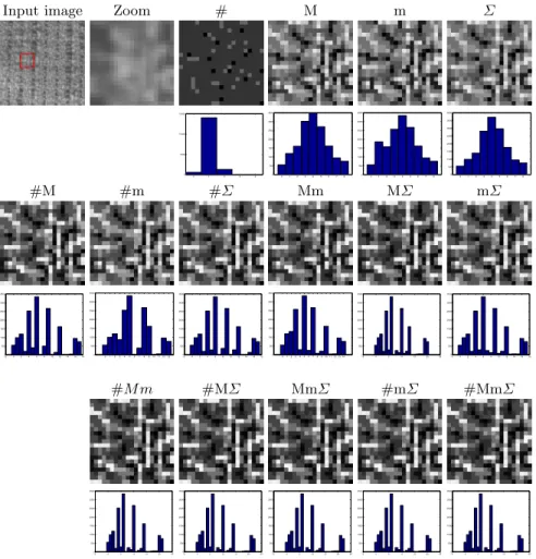
In the experiments, we shall denote the texture descriptor based on the subset of attributes A as LBPA_P,R, following the conventional notations u2 or riu2 in LBP based models. Figure 2 shows a texture image with its corresponding label images and label histograms for the different configurations of LBPA1,8. In addition,

Figure 3 shows images and histograms of labels corresponding to LBP#M m_1,8 for different images, from the same texture class (first row), and from different classes (second row). The visual (di)similarity of histograms depending on the class is apparent on the figure.

To assess the interest of differentiating uniform patterns or not, a mixed texture representation (LBPriu2+A_P,R ) is also evaluated in our work, by taking into account the above encoding only on non-uniform patterns, and using riu2 encoding for uniform patterns:

LBPriu2+A_P,R (p) = (

LBPriu2_P,R(p), if LBPP,R(p) is uniform

p + 1 + Λ (LBPP,R(p)) , otherwise

3.3 Relation with previous works

As mentioned before, LBPA_P,Rare related with other rotation invariant patterns: LBPriu2_P,R [2] and LBC [12]. We now discuss further those relations.

– LBPΣ

P,R is exactly LBC. It means that if Σ ∈ A, LBPAP,R is a generalisation

of LBC.

– When card(A) ≥ 2 and (# ∈ A or Σ ∈ A), LBPA_P,Ris a superset of LBPriu2 P,R

patterns. In that case indeed, riu2 patterns are distinguished, either by the value of # and anyone among {M, m, Σ}, or by one of the identity M = Σ or

m = Σ.1 _{Therefore, for such combination of attributes A, LBP}A

P,R inherits

the distinctive properties of LBPriu2

P,R , while containing more information. In

this sense, LBP_P,RA generalises LBPriu2_P,R.

– As a consequence, with the same conditions on A, the performance of LBPA_P,R and LBPriu2+A_P,R are the same.

– When card(A) = 1 or A = {M, m}, A and riu2 are complementary, and LBPriu2+A_P,R can be better than LBPA_P,R or LBPriu2

P,R alone.

Table 1 displays the number of labels (and then of histogram bins) for the different configurations of attributes. Note that the numbers for LBPA

P,R and

LBPriu2+A_P,R are different only if card(A) = 1 or A = {M, m}. In addition, Table 2 shows the number of labels for several existing LBP-based methods.

Table 1. Number of different labels, i.e. number of histogram bins of the texture

descriptor in the different configurations.

Schema # M m Σ M# m# MΣ Mm #Σ mΣ Mm# #MΣ MmΣ #mΣ #MmΣ LBPA_8,1 5 9 9 9 18 14 21 15 18 18 22 23 23 22 23 LBPA_16,2 9 17 17 17 66 36 92 59 66 66 125 180 159 125 212 LBPA_24,3 13 25 25 25 146 62 225 135 146 146 353 680 557 353 989 LBPriu2+A_8,1 12 14 14 14 18 14 21 18 18 18 22 23 23 22 23 LBPriu2+A_16,2 24 30 30 30 66 36 92 66 66 66 125 180 159 125 212 LBPriu2+A_24,3 36 46 46 46 146 62 225 146 146 146 353 680 557 353 989

Table 2. Number of different labels in several encodings.

Method (P,R)=(8,1) (P,R)=(16,2) (P,R)=(24,3) LBPriu2_P,R 10 18 26 LBPu2

P,R 59 243 555

CLBPriu2_P,R 200 648 1352

There is a strong link between LBPriu2+A_P,R with previous works aiming at exploiting information from non-uniform patterns to improve the texture de-scriptors. In particular LBPriu2+{Σ}_P,R and LBPriu2+{#}_P,R are close to [14]. In this work, the authors extended the notion of uniform pattern (as the Σ attribute does), and the other patterns were encoded by the number of 0-1 transitions, which corresponds to the # attribute.

3.4 Completed texture descriptor

Guo et al [11] proposed a state-of-the-art variant of LBP by coding the local differences as two complementary components: signs (sp= s(gp− gc)) and

mag-nitudes (mp = |gp − gc|). They proposed to use two binary patterns, called

1

Note that {M, m} alone do not allow to distinguish uniform patterns, since the identity M = m can occur with several connected components.

Input image Zoom # M m Σ 0 1 2 3 4 0 5000 10000 15000 0 1 2 3 4 5 6 7 8 0 500 1000 1500 2000 2500 3000 3500 0 1 2 3 4 5 6 7 8 0 500 1000 1500 2000 2500 3000 3500 0 1 2 3 4 5 6 7 8 0 500 1000 1500 2000 2500 3000 3500 4000 #M #m #Σ Mm MΣ mΣ −2 0 2 4 6 8 1012141618 0 500 1000 1500 2000 2500 3000 3500 012345678910111213 0 500 1000 1500 2000 2500 3000 3500 −2 0 2 4 6 8 1012141618 0 500 1000 1500 2000 2500 3000 3500 01234567891011121314 0 500 1000 1500 2000 2500 3000 3500 −5 0 5 10 15 20 25 0 500 1000 1500 2000 2500 3000 3500 −2 0 2 4 6 8 1012141618 0 500 1000 1500 2000 2500 3000 3500 #M m #MΣ MmΣ #mΣ #MmΣ −5 0 5 10 15 20 25 0 500 1000 1500 2000 2500 3000 3500 −5 0 5 10 15 20 25 0 500 1000 1500 2000 2500 3000 3500 −5 0 5 10 15 20 25 0 500 1000 1500 2000 2500 3000 3500 −5 0 5 10 15 20 25 0 500 1000 1500 2000 2500 3000 3500 −5 0 5 10 15 20 25 0 500 1000 1500 2000 2500 3000 3500

Fig. 2. A texture image and its label images and label histograms for the different configurations of attributes, with (P, R) = (8, 1). For the best visualization, the label images are zoomed from a part corresponding to the red square of the texture image.

−5 0 5 10 15 20 25 0 500 1000 1500 2000 2500 3000 3500 −5 0 5 10 15 20 25 0 500 1000 1500 2000 2500 3000 3500 −5 0 5 10 15 20 25 0 500 1000 1500 2000 2500 3000 3500 −5 0 5 10 15 20 25 0 500 1000 1500 2000 2500 −5 0 5 10 15 20 25 0 500 1000 1500 2000 2500 3000 3500 −5 0 5 10 15 20 25 0 500 1000 1500 2000 2500

Fig. 3. Texture images and their label images and histograms for LBP#M m_8,1 . The first

CLBP-Sign (CLBP S) and CLBP-Magnitude (CLBP M). The first pattern is identical to the LBP. The second one which measures the local variance of mag-nitude is defined as follows:

CLBP MP,R= P −1

X

p=0

s(mp− ˜m).2p,

where ˜m is the mean value of mp for the whole image. In addition, Guo et

al. observed that the local value itself carries important information. Therefore, they defined the operator CLBP-Center (CLBP C) as follows:

CLBP C = s(gc− ˜g),

where ˜g is the mean gray level for the whole image. Because these operators are complementary, their combination leads to a significant improvement, and then CLBP is now considered a reference method in texture classification.

Inspired from this work, we also evaluated our descriptors by complementing the difference sign information (CLBP S) by the difference magnitude (CLBP M) and gray level (CLBP C). For CLBP S and CLBP M, instead of using riu2 map-ping, we apply our proposed encoding to obtain CLBPA

P,R and CLBP MAP,R.

Finally, the feature vector of the whole image is constructed by considering the joint histograms of CLBP SA_P,R, CLBP MA_P,Rand CLBP C. Then, if LBPA_P,Rhas n different labels, CLBPA

P,R has 2n

2 _{labels (see also Table 1).}

3.5 Texture classification

Because the contribution of this work is focused on texture descriptors, and the competing LBP based methods all used χ2 _{distance as similarity metrics [2],}

and nearest neighbour as classification criterion, we used the same classification method for fair comparison purposes. If H1 and H2 are two attribute label

histograms, the χ2_{-dissimilarity between the two textures is:}

χ2(H1, H2) = N X i=1 (H1(i) − H2(i))2 H1(i) + H2(i) ,

with N = NAor N = Nriu2+A the number of labels.

4

Experiments

4.1 Datasets

The effectiveness of the proposed method is assessed by a series of experiments on three large and representative databases: Outex [15], CUReT [16] and UIUC [17]. The Outex database (examples are shown in Figure 6) contains images cap-tured from a wide variety of real materials. We consider the two commonly used test suites, Outex TC 00010 (TC10) and Outex TC 00012 (TC12), containing

24 classes of textures. Each image may be seen under nine different rotation an-gles between 0 and 90◦. For TC10, The texture images at angle 0◦are chosen for training the classifier, all the remaining images are used for testing. For TC12, aside from the different viewing angles, the images can have three types of il-lumination: “inca”, used for learning, and “t184” or “horizon”, used for testing (test sets are denoted TC12t and TC12h respectively).

Fig. 4. Texture images with the illumination condition “inca” and zero degree rotation angle from the 24 classes of textures on the Outex database.

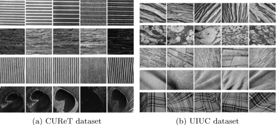
The CUReT database contains 61 texture classes (see Figure 5.a), each having 205 images acquired at different viewpoints and illumination orientations. We follow the experimental protocol proposed in [18, 19], using 4 different learning sets made of 6, 12, 23 and 46 images (first line of Table 7).

(a) CUReT dataset (b) UIUC dataset

Fig. 5. Examples of texture images.

The UIUC texture database includes 25 classes with 40 images in each class. The resolution of each image is 640×480. The database contains materials

im-aged under significant viewpoint variations (examples are shown in Figure 5.b). Following [17], to eliminate the dependence of the results on the particular train-ing images used, four different learntrain-ing sets of 5, 10, 15 and 20 images are used while the remaining images per class are used as test set.

In the upcoming result sections, the performance measure will be given in percentage of correct classification. As the typical size of the test sets is around 5 000, the percentage values are rounded to the first decimal. Furthermore, our methods is practically deterministic (ignoring the slight influence of interpolation in the computation of the LBP). Finally, the test protocol of the Outex dataset is also deterministic, and the typical observed standard deviation in the cross validation schemes of Curet and UIUC is less than 0.1%.

4.2 Computational cost

We consider in this section the computational cost of our descriptors with respect to other LBP-based operators. Experiments on Outex TC10 test suite containing 4320 images of 128 × 128 pixels were performed on a machine with 2.0 GHz CPU, 4Go RAM and Linux 3.2.0-23 kernel. Table 3 presents the computation time (in seconds) of different descriptors in the configuration (P, R) = (2, 16) and reports the total time (in seconds) for classifying the 3840 test images against the 480 reference images.

Table 3. Complexity of our different descriptors with respect to LBPriu2(FET:

Fea-ture Extraction Time, MT: Matching Time).

Method riu2 # M m Σ M# m# MΣ Mm #Σ mΣ Mm# #MΣ MmΣ #mΣ #MmΣ FET 78.1 79.2 78.4 78.3 80.2 80.9 80.8 79.2 78.7 79.5 78.9 80.3 80.6 83.3 83.3 82.2

MT 1.2 0.9 1.1 1.1 1.2 4.7 2.1 4.7 2.7 4.5 3.2 6.9 11.4 10.1 6.5 13.1

As can be seen from Table 3, the descriptor construction time does not vary much from one method to the other, while the classification time is proportional to the length of the feature vector.

4.3 1st experiment: LBPA_P,R and LBPriu2+A_P,R

Table 4 compares our descriptors (LBPA_P,R) with the classic LBPriu2

P,R on Outex

dataset, for different (P, R) configurations. Those results can be interpreted as follows:

– The four attributes have distinct properties. Considered alone, their perfor-mance is comparable to LBPriu2

P,R, except for #, whose expressiveness is too

weak if taken alone.

– Jointly considering 2 attributes, the results are (except in one case) better than LBPriu2

Method (P,R)=(8,1) (P,R)=(16,2) (P,R)=(24,3) TC10 TC12 t TC12 h Mean TC10 TC12 t TC12 h Mean TC10 TC12 t TC12 h Mean LBPriu2_{[2] 84.8 65.5 63.7 71.3 89.4 82.3 75.2 82.3 95.1 85.0 80.8 87.0} LBP# _{52.4 37.4 32.0 40.6 66.5 51.3 47.1 55.0 77.0 67.5 58.2 67.6} Gain - - - -LBPM 83.6 67.1 64.4 71.7 87.6 82.2 78.9 82.9 95.9 88.1 86.4 90.1 Gain - 1.6 0.7 0.4 - - 3.7 0.6 0.8 3.1 5.6 3.1 LBPm _{84.8 64.5 62.2 69.9 91.0 82.9 77.0 83.7 96.5 86.2 80.4 87.7} Gain 0.0 - - - 1.6 0.6 1.8 1.4 1.4 1.2 - 0.7 LBPΣ _{82.9 65.0 63.2 70.4 88.7 82.6 77.4 82.9 91.3 83.8 82.7 86.0} Gain - - - 0.3 2.2 0.6 - - 1.9 -LBPM # 86.5 69.9 66.2 74.2 93.7 85.3 82.1 87.1 96.8 88.7 84.3 89.9 Gain 1.7 4.4 2.5 2.9 4.3 3.0 6.9 4.8 1.7 3.7 3.5 2.9 LBPm# 85.7 67.4 66.4 73.1 93.1 85.9 81.4 86.8 97.5 89.3 85.0 90.6 Gain 0.9 1.9 2.7 1.8 3.7 3.6 6.2 4.5 2.4 4.3 4.2 3.6 LBPM Σ _{85.8 69.7 66.6 74.0 92.5 85.9 82.3 86.9 96.9 89.9 86.0 91.0} Gain 1.0 4.2 2.9 2.7 3.1 3.6 7.1 4.6 1.8 4.9 5.2 4.0 LBPM m _{85.6 66.8 63.6 72.0 92.5 85.4 82.4 86.8 98.1 92.2 87.2 92.5} Gain 0.8 1.3 - 0.7 3.1 3.1 7.2 4.5 3.0 7.2 6.4 5.5 LBP#Σ _{87.1 69.8 67.8 74.9 93.4 84.6 79.7 85.9 96.5 87.5 83.6 89.2} Gain 2.3 4.3 4.1 3.6 4 2.3 4.5 3.6 1.4 2.5 2.8 2.2 LBPmΣ 86.0 70.1 66.8 74.3 92.9 85.8 83.4 87.4 97.8 91.4 86.8 92.0 Gain 1.2 4.6 3.1 3.0 3.5 3.6 8.2 5.1 2.7 6.4 6.0 5.0 LBPM m# 85.8 70.5 68.2 74.8 94.3 86.8 84.2 88.4 97.2 90.9 86.7 91.6 Gain 1.0 5.0 4.5 3.5 4.9 3.5 9.0 6.1 2.1 5.9 5.9 4.6 LBP#M Σ _{86.0 70.6 67.9 74.8 93.7 87.0 84.3 88.3 97.2 90.4 86.2 91.3} Gain 1.2 5.1 4.2 3.5 4.3 4.7 9.1 6.0 2.1 5.4 5.4 4.3 LBPM mΣ _{86.0 70.6 67.9 74.8 94.1 87.3 84.1 88.5 97.0 90.3 86.4 91.2} Gain 1.2 5.1 4.2 3.5 4.7 5.0 8.9 6.2 1.9 5.3 5.6 4.2 LBP#mΣ _{86.1 70.8 67.8 74.9 94.1 87.0 84.1 88.4 97.4 91.0 86.7 91.7} Gain 1.3 5.3 4.1 3.6 4.7 4.7 8.9 6.1 2.3 6.0 5.9 4.7 LBP#M mΣ 86.0 70.6 67.9 74.8 94.1 87.6 84.5 88.7 97.1 90.2 86.4 91.2 Gain 1.2 5.1 4.2 3.5 4.7 5.3 9.3 6.4 2.0 5.2 5.6 4.2

Table 4. Comparison between LBPriu2and the basic LBPA on Outex dataset.

– Using 3 or 4 attributes further improves the results, except when P = 24. This can be explained by the fact that in this case, the number of labels is too high, which makes the histogram too sparse for the χ2 _distance.

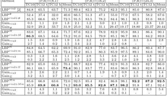
In addition, Table 5 presents a comparison between LBPriu2+A_P,R and LBPriu2 P,R,

when A is mono attribute or {M m}. It can be seen that the performance of LBPriu2+A_P,R is, in most cases, better than LBPA_P,R or LBPriu2

P,R alone.

4.4 2nd experiment: CLBPA_P,R

Because, when the number of labels become too large (P = 24), the use of several attributes become really inefficient due to the very high dimension of feature vectors, in this experiment we consider only a combination of at most two attributes.

Table 6, 7, 8 present the results obtained by our methods CLBPA_P,R on the three datasets (Outex, CUReT and UIUC) in comparison with other LBP-based methods. From these tables, we can make the following remarks

Method (P,R)=(8,1) (P,R)=(16,2) (P,R)=(24,3) TC10 TC12 t TC12 h Mean TC10 TC12 t TC12 h Mean TC10 TC12 t TC12 h Mean LBPriu2_{[2] 84.8 65.5 63.7 71.3 89.4 82.3 75.2 82.3 95.1 85.0 80.8 87.0} LBP# _{52.4 37.4 32.0 40.6 66.5 51.3 47.1 55.0 77.0 67.5 58.2 67.6} LBPriu2+# _{85.3 66.6 65.7 72.5 91.5 83.5 78.2 84.4 96.1 86.3 81.6 88.0} Gainriu2 0.5 1.1 2.0 1.3 2.1 1.2 3.0 2.1 1.0 1.3 0.8 1.0 Gain# 32.9 29.2 33.7 31.9 25.0 32.2 31.1 29.47 19.17 18.80 23.37 20.44 LBPM 83.6 67.1 64.4 71.7 87.6 82.2 78.9 82.9 95.9 88.1 86.4 90.1 LBPriu2+M 86.3 68.5 64.6 73.2 91.0 84.5 79.9 85.1 96.7 88.1 84.2 89.8 Gainriu2 1.5 3.0 0.9 1.9 1.6 2.2 4.7 2.8 1.6 3.1 3.4 2.8 GainM 2.7 1.4 0.2 1.5 3.4 2.3 1.0 2.2 0.8 - - -LBPm _{84.8 64.5 62.2 69.9 91.0 82.9 77.0 83.7 96.5 86.2 80.4 87.7} LBPriu2+m _{85.1 66.7 65.3 72.4 92.2 85.1 80.3 85.9 97.5 89.1 84.6 90.0} Gainriu2 0.3 1.2 1.6 1.1 2.8 2.8 5.1 3.6 2.4 4.1 3.8 3.0 Gainm 0.3 2.2 3.1 2.5 1.2 2.2 3.3 2.2 1.0 2.9 4.2 2.3 LBPΣ _{82.9 65.0 63.2 70.4 88.7 82.6 77.4 82.9 91.3 83.8 82.7 86.0} LBPriu2+Σ 86.1 68.1 65.9 73.4 90.1 83.7 77.1 83.6 96.0 86.3 82.8 88.4 Gainriu2 1.3 2.6 2.2 2.1 0.7 1.4 1.9 1.3 0.9 1.3 2.0 1.4 GainΣ 3.2 3.1 2.7 3.0 1.4 1.1 - 0.7 4.7 2.5 0.1 2.4 LBPM m 85.6 66.8 63.6 72.0 92.5 85.4 82.4 86.8 98.1 92.2 87.2 92.5 LBPriu2+M m _{85.9 69.8 66.8 74.2 93.0 85.5 82.8 87.1 98.2 91.8 87.1 92.4} Gainriu2 1.1 4.3 1.1 2.9 3.6 3.2 7.6 4.8 3.1 6.8 6.3 5.4 GainM m 0.3 3.0 3.2 2.2 0.5 0.1 0.4 0.3 0.1 - -

-Table 5. Comparison between LBPriu2, LBPAand the mixed LBPriu2+A on Outex

dataset when A is a mono attribute or {M m}.

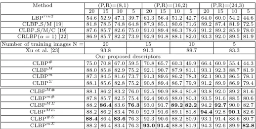
– Except when A = {#}, CLBPA_P,R outperforms the previous methods in all configurations.

– Between mono attributes, M is the best configuration. It means that CLBPM

outperforms CLBC [12] that is exactly CLBPΣ_.

– The combination of two attributes still improves the performance of our descriptors. The improvement in relation with CLBP S/M/C varies from 0.5% to 4.5% depending on test configurations.

In addition, Figure 6 presents the best results of one configuration (M #) in comparison with the best results of recent methods on Outex dataset: LBPriu2 [2], LTP [7], DLBP + NGF [10], VZ-MR8 [20], VZ-Joint [20], CLBP S M/C [11] and CLBP CLBC [12]. As can be seen from it, because the topology-related attributes bring more information than the typical mapping riu2, our best results in complementary scheme improve significantly with respect to CLBP.

5

Conclusions

We have proposed a versatile and efficient variant of LBP for texture description. The proposed framework extends existing rotation invariant LBP based coding, including riu2 and LBC, while enhancing their expressiveness and improving their discrimination capability. The classification results on three recent texture datasets prove the relevance of our framework. Used in combination with the

2

Method (P,R)=(8,1) (P,R)=(16,2) (P,R)=(24,3) TC10 TC12 t TC12 h Mean TC10 TC12 t TC12 h Mean TC10 TC12 t TC12 h Mean LBPriu2_{[2] 84.8 65.5 63.7 71.3 89.4 82.3 75.2 82.3 95.1 85.0 80.8 87.0} LTP [7] 94.1 75.9 74.0 81.3 97.0 90.2 86.9 91.3 98.2 93.6 89.4 93.8 DLBP [10] 97.7 92.1 88.7 92.8 98.1 91.6 87.4 92.4 DLBP + NGF [10] 99.1 93.2 90.4 94.2 98.2 91.6 87.4 92.4 CLBP S M/C [11] 94.5 81.9 82.5 86.3 98.0 91.0 91.1 93.4 98.3 94.0 92.4 94.9 CLBP S/M [11] 94.7 82.7 83.1 86.8 97.9 90.5 91.1 93.2 99.3 93.6 93.3 95.4 CLBP S/M/C [11] 96.6 90.3 92.3 93.0 98.7 93.5 93.9 95.4 98.9 95.3 94.5 96.3

Our proposed descriptors

CLBP# 85.4 71.7 70.7 75.9 90.6 83.4 80.9 85.0 89.0 81.3 79.3 83.2 CLBPM 96.5 90.9 93.0 93.4 98.4 95.5 96.2 96.7 99.1 97.2 96.8 97.7 CLBPm _{96.7 90.5 91.6 92.9 99.0 95.6 94.9 90.5 99.5 96.7 96.0 97.4} CLBPΣ _{97.2 89.8 92.9 93.3 98.5 93.3 94.1 95.3 98.8 94.0 95.4 96.1} CLBPM # 96.2 90.6 93.5 93.5 98.9 95.5 95.8 96.8 99.5 97.0 96.3 97.6 CLBPm# 96.3 90.4 92.2 93.0 98.9 95.3 95.1 96.4 99.3 96.4 96.0 97.2 CLBPM Σ 96.3 91.1 93.4 93.6 98.9 95.3 96.5 96.9 99.4 94.3 93.4 95.7 CLBPM m _{96.8 90.9 93.2 93.6 98.9 95.7 95.2 96.6 99.3 95.5 93.8 96.2} CLBP#Σ _{96.7 90.7 93.6 93.6 99.0 95.4 96.1 96.8 99.6 96.2 95.8 97.2} CLBPmΣ _{96.5 90.6 92.3 93.1 99.0 95.23 96.1 96.8 99.1 94.6 93.0 95.5}

Table 6. Comparison between CLBPAP,R and other LBP-based methods on Outex

dataset.

complemented LBP coding, it even outperforms the state-of-the art LBP based descriptors. In the future, we plan to address the problem of high dimensionality when using more attributes in complemented LBPs.

References

1. T. Ojala, M. Pietik¨ainen, and D. Harwood, “A comparative study of texture

measures with classification based on featured distributions,” Pattern Recognition, vol. 29(1), pp. 51–59, 1996.

2. T. Ojala, M. Pietik¨ainen, and T. M¨aenp¨a¨a, “Multiresolution gray-scale and

ro-tation invariant texture classification with local binary patterns,” IEEE Trans. PAMI, vol. 24, pp. 971–987, 2002.

Outex_TC_00010 Outex_TC_00012 (tl84) Outex_TC_00012 (horizon) 80 82 84 86 88 90 92 94 96 98 100 99,5 97 _96,3 92 _91,4 92 93,6 92,6 92,8 99,1 93,2 90,4 97,8 95,4 95,6 99 95,4 _94,7 95,1 85 80,8 98,9 95,3 94,5

Ours VZ-Joint VZ-MR8 DLBP&NGF LBPV CLBP_CLBC LBP CLBP_S/M/C

C la ss if ic a ti o n A cc u ra cy (% )

Fig. 6. Comparing the best results of CLBPM #with the best results of recent methods

Method (P,R)=(8,1) (P,R)=(16,3) (P,R)=(24,5) N=46 N=23 N=12 N=6 N=46 N=23 N=12 N=6 N=46 N=23 N=12 N=6 LTP [7] 85.13 79.25 72.25 63.09 92.66 87.30 80.22 70.50 91.81 85.78 77.88 67.77 LBPriu2/VARP,R[21] 93.87 88.76 81.59 71.03 94.20 89.12 81.64 71.81 91.87 85.58 77.13 66.04 CLBP S/M/C [11] 95.6 91.3 84.9 74.8 95.9 92.1 86.1 77.0 94.7 90.3 83.8 74.5 CLBP S/M [11] 93.5 88.7 81.9 72.3 94.4 90.4 84.2 75.4 93.6 89.1 82.5 73.3

Our proposed descriptors

CLBP# _{81.8 72.2 61.8 52.0 82.3 72.8 61.6 50.2 77.7 67.6 56.5 45.2} CLBPM _{95.7 91.5 84.1 74.0 96.1 92.5 85.7 76.3 96.4 92.3 85.9 77.6} CLBPm 95.8 91.3 83.8 73.7 96.8 92.5 85.8 77.1 95.4 91.6 85.4 77.8 CLBPΣ _{94.8 90.1 82.7 72.1 94.7 89.8 82.3 72.0 93.9 87.5 80.6 69.0} CLBPm# _{95.9 91.7 84.4 74.5 97.0 93.2 86.7 78.2 96.1 92.6 85.9 78.6} CLBPM Σ _{96.3 92.1 84.8 74.8 96.0 92.0 85.7 76.5 x x x x} CLBPM m 96.2 91.9 84.7 74.6 96.7 93.1 86.7 78.1 94.5 90.45 83.8 77.0 CLBP#Σ 96.2 91.8 84.6 74.8 96.5 92.7 86.2 77.1 93.7 89.0 81.5 73.8 CLBPmΣ _{96.3 91.9 84.9 74.4 96.7 92.5 86.7 77.1 92.27 88.1 80.6 73.7} CLBPM # _{96.3 92.1 84.7 75.1 96.8 93.2 87.3 78.2 95.01 91.2 84.24 77.1}

Table 7. Experimentation of CLBPAP,Ron CUReT dataset

2

.

3. Pietikinen Matti, Hadid Abdenour, Zhao Guoying, and Ahonen Timo, Computer Vision Using Local Binary Patterns, 2011.

4. Wenchao Zhang, Shiguang Shan, Wen Gao, Xilin Chen, and Hongming Zhang, “Lo-cal Gabor Binary Pattern Histogram Sequence (LGBPHS): A Novel Non-Statisti“Lo-cal Model for Face Representation and Recognition,” in ICCV, 2005, pp. 786–791. 5. Shu Liao and Albert C. S. Chung, “Face recognition by using elongated local

binary patterns with average maximum distance gradient magnitude,” in ACCV, Yasushi Yagi, Sing Bing Kang, In-So Kweon, and Hongbin Zha, Eds., 2007, vol. 4844 of LNCS, pp. 672–679.

6. L. Wolf, T. Hassner, and Y. Taigman, “Descriptor based methods in the wild,” in Real-Life Images Workshop, ECCV, 2008.

7. Xiaoyang Tan and Bill Triggs, “Enhanced local texture feature sets for face recog-nition under difficult lighting conditions,” IEEE Trans. Image Processing, vol. 19, no. 6, pp. 1635–1650, 2010.

8. M¨aenp¨a¨a T. and Pietik¨ainen M., “Multi-scale binary patterns for texture analysis,”

in SCIA, 2003, vol. 2749 of LNCS, pp. 885–892.

9. S.C. Liao, X.X. Zhu, Z. Lei, L. Zhang, and S.Z. Li, “Learning multi-scale block local binary patterns for face recognition,” in ICB, 2007, vol. 4642 of LNCS, pp. 828–837.

10. S. Liao, M. W. K. Law, and A. C. S. Chung, “Dominant local binary patterns for texture classification,” IEEE Trans. Image Processing, vol. 18, no. 5, pp. 1107– 1118, May 2009.

11. Guo Z., Zhang Z., and Zhang D., “A completed modeling of local binary pattern operator for texture classification,” IEEE Trans. Image Processing, vol. 19(6), pp. 1657–1663, 2010.

12. Yang Zhao, De-Shuang Huang, and Wei Jia, “Completed local binary count for rotation invariant texture classification,” IEEE Trans. Image Processing, vol. 21, no. 10, pp. 4492–4497, 2012.

13. Shigeki Yokoi, Jun-Ichiro Toriwaki, and Teruo Fukumura, “An analysis of topo-logical properties of digitized binary pictures using local features,” CGIP, vol. 4, pp. 63–73, 1975.

Method (P,R)=(8,1) (P,R)=(16,2) (P,R)=(24,3) 20 15 10 5 20 15 10 5 20 15 10 5 LBPriu2 _{54.6 52.9 47.1 39.7 61.3 56.4 51.2 42.7 64.0 60.0 54.2 44.6} CLBP S/M [19] 81.8 78.5 74.8 64.8 87.9 85.1 80.6 71.6 89.2 87.4 81.9 72.5 CLBP S/M/C [19] 87.6 85.7 82.6 75.0 91.0 89.4 86.3 78.6 91.2 89.2 85.9 78.0 CRLBP(α = 1) [22] 86.9 85.7 82.2 73.9 92.9 91.8 88.1 82.0 93.3 92.0 89.5 81.9 Number of training images N = 20 15 10 5

Xu et al. [23] 93.8 91.3 89.7 83.3 Our proposed descriptors

CLBP# _{75.0 70.8 67.0 59.5 70.8 65.7 60.3 49.9 66.4 60.9 55.4 44.3} CLBPM _{88.0 85.8 82.9 75.2 92.1 90.7 87.9 81.1 93.1 92.3 88.7 81.9} CLBPm 87.3 84.5 81.6 73.7 91.3 89.6 86.2 78.3 92.1 90.3 86.5 78.1 CLBPΣ _{88.1 85.6 82.8 75.2 90.8 89.4 86.7 79.9 91.2 89.9 86.9 79.4} CLBPM # _{88.1 86.2 83.2 76.0 92.5 90.9 88.4 80.8 93.8 92.0 89.2 81.6} CLBPm# _{87.8 85.7 82.5 75.4 92.4 90.6 88.0 80.3 93.5 91.6 88.5 80.6} CLBPM Σ _{88.2 86.4 83.6 76.3 93.0 91.7 89.2 82.2 94.2 92.7 90.0 82.7} CLBPM m 88.2 86.2 83.4 76.0 92.9 91.6 89.1 81.8 94.4 92.8 90.1 82.6 CLBP#Σ 88.4 86.4 83.6 76.3 92.3 90.6 88.2 80.9 93.1 91.4 88.6 80.7 CLBPmΣ _{88.2 86.4 83.4 76.3 93.0 91.4 88.8 81.9 94.3 92.6 89.9 82.8}

Table 8. Experimentation of CLBPAP,Ron UIUC dataset.

14. Abdolhossein Fathi and Ahmad Reza Naghsh-Nilchi, “Noise tolerant local binary pattern operator for efficient texture analysis,” Pattern Recognition Letters, vol. 33, no. 9, pp. 1093–1100, 2012.

15. Timo Ojala, Topi Menp, Matti Pietikinen, Jaakko Viertola, Juha Kyllnen, and Sami Huovinen, “Outex - new framework for empirical evaluation of texture anal-ysis algorithms,” in ICPR, 2002, pp. 701–706.

16. Kristin J. Dana, Bram van Ginneken, Shree K. Nayar, and Jan J. Koenderink, “Reflectance and texture of real-world surfaces,” ACM Trans. Graph., vol. 18, pp. 1–34, 1999.

17. S. Lazebnik, C. Schmid, and J. Ponce, “A sparse texture representation using local affine regions,” IEEE Trans. PAMI, vol. 27, no. 8, pp. 1265–1278, 2005.

18. Manik Varma and Andrew Zisserman, “A statistical approach to material classi-fication using image patch exemplars,” IEEE Trans. PAMI, vol. 31, no. 11, pp. 2032–2047, 2009.

19. Zhenhua Guo, Lei Zhang, and D. Zhang, “A completed modeling of local binary pattern operator for texture classification,” IEEE Trans. Image Processing, vol. 19, no. 6, pp. 1657–1663, June 2010.

20. Manik Varma and Andrew Zisserman, “A statistical approach to texture classifi-cation from single images,” International Journal of Computer Vision, vol. 62, no. 1-2, pp. 61–81, 2005.

21. T. Ojala, M. Pietikainen, and T. Maenpaa, “Multiresolution gray-scale and ro-tation invariant texture classification with local binary patterns,” IEEE Trans. PAMI, vol. 24, no. 7, pp. 971–987, July 2002.

22. Yang Zhao, Wei Jia, Rong-Xiang Hu, and Hai Min, “Completed robust local binary pattern for texture classification,” Neurocomputing, vol. 106, pp. 68–76, 2013.

23. Yong Xu, Hui Ji, and Cornelia Ferm¨uller, “Viewpoint invariant texture description

using fractal analysis,” International Journal of Computer Vision, vol. 83, no. 1, pp. 85–100, 2009.