Trajectory Generation for a Quadrotor Unmanned Aerial Vehicle

TRAJECTORY GENERATION FOR A QUADROTOR UNMANNED AERIAL VEHICLE

DOUGLAS CONOVER

DÉPARTEMENT DE GÉNIE ÉLECTRIQUE ÉCOLE POLYTECHNIQUE DE MONTRÉAL

MÉMOIRE PRÉSENTÉ EN VUE DE L’OBTENTION DU DIPLÔME DE MAÎTRISE ÈS SCIENCES APPLIQUÉES

(GÉNIE ÉLECTRIQUE) SEPTEMBRE 2018

ÉCOLE POLYTECHNIQUE DE MONTRÉAL

Ce mémoire intitulé :

TRAJECTORY GENERATION FOR A QUADROTOR UNMANNED AERIAL VEHICLE

présenté par : CONOVER Douglas

en vue de l’obtention du diplôme de : Maîtrise ès sciences appliquées a été dûment accepté par le jury d’examen constitué de :

M. GOURDEAU Richard, Ph. D., président

M. SAUSSIÉ David, Ph. D., membre et directeur de recherche M. ACHICHE Sofiane, Ph. D., membre

DEDICATION

To Granddad, With every passing year I see more of you in me but never enough to hand-cut a sunroof into my new car.

ACKNOWLEDGMENTS

I would like to thank my supervisor David Saussié, who two years ago gave me the chance to pursue my budding interest in aerospace and control. I would also like to acknowledge André Phu-Van Nguyen and Olivier Gougeon, who aided me in the experimental implementation of my work. Your knowledge of the lab and willingness to help when I hit a dead-end unquestio-nably saved me from hours of frustration. Thank you to Tien Nguyen, who was always there to entertain my questions and help with any theoretical issues I had. Thanks also to Justin Cano, your energy and enthusiasm was welcome every day I spent in the lab. Thank you to Maeve Reimer and Jorge Zavagno who helped me produce the composite photos found in this work.

Thank you to Pierre, Hugo, Vincent, Tangui, Clément, Adriel and the rest of the 4th floor lab for your lightheartedness and help throughout my Master’s. When courses seemed overw-helming, I could always count on one of you for explanation and guidance.

Finally, I would like to thank my family for their love and support over the course of this degree. To my parents Cecilia and Kent, you kept me going with Sunday dinners and tup-perwares full of pancakes. Thank you to my grandparents Paul and Betty, who supported me and never stopped encouraging me to follow my interests. Thank you to Cort, Sue, Eric, Richard and Ann-Margrit, who were always curious to hear where my studies were taking me. To my sister Rachel, who is still the only one who will watch scary movies with me. To my brother Jared, who won’t watch scary movies, but is always willing to toss a frisbee around. I love you all.

RÉSUMÉ

Le domaine des véhicules aériens sans pilote de type multicoptères a connu une progression substantielle au cours de la dernière décennie. La génération et le contrôle des trajectoires ont été au centre des préoccupations de ce nouveau domaine, avec des méthodes qui permettent d’exécuter des manœuvres complexes dans l’espace. Plusieurs efforts ont été faits pour exé-cuter ces manœuvres en utilisant la commande non linéaire, notamment la commande par platitude différentielle. Cependant, l’absence de théorie pour l’estimation des dérivées d’ordre supérieur a empêché l’application expérimentale de plusieurs de ces techniques.

Ce travail explore tout d’abord l’approche par composition séquentielle pour l’exécution de manœuvres à travers des fenêtres étroites. Cette technique implique la combinaison de plu-sieurs contrôleurs théoriquement simples afin de produire un résultat complexe. Les résultats expérimentaux réalisés dans le Laboratoire de Robotique Mobile et de Systèmes Automati-sés à Polytechnique Montréal démontrent la validité de cette approche, en produisant des manœuvres précises et répétables. Cependant, on atteint rapidement les limites d’une telle méthode dans les applications du monde réel, du fait de son manque de précision initiale et l’absence d’évaluation de faisabilité.

Ce mémoire se concentre ensuite sur le développement d’une architecture d’estimation d’état basée sur le filtre de Kalman linéaire afin de fournir en temps réel des estimés des 2e _et

3e _{dérivées de la position d’un quadricoptère (appelées respectivement accélération, et}

à-coup ou jerk). Des filtres de complexités différentes sont développés afin d’incorporer toute l’information disponible sur le système pour améliorer l’estimé résultant. On obtient alors un estimateur d’état complet qui utilise les mesures de position et d’accélération, ainsi que les entrées de commande, et fournit des estimés pour la rétroaction. Un contrôleur du jerk augmenté basé sur la théorie de la commande optimale est ensuite développé afin de valider cet estimateur. Il est conçu de façon à utiliser le jerk, l’accélération, la vitesse et la position du drone ; sans rétroaction de chacun de ces termes, le système est alors instable. Des tests sont effectués afin d’examiner les performances de l’estimateur et du contrôleur. Tout d’abord, le quadricoptère est chargé de suivre diverses entrées de référence dans l’espace pour assurer sa stabilité. Le contrôleur permet de suivre au plus près ces références, comme réalisé en simulation. Le contrôleur doit ensuite suivre un changement de référence afin d’évaluer la précision de l’estimateur développé. Les résultats montrent que l’estimation en temps réel du jerk suit adéquatement les valeurs hors ligne. Pour autant que nous le sachions, c’est la première mise en œuvre dans le monde réel du retour de jerk pour contrôler un multicoptère.

ABSTRACT

The field of multirotor unmanned aerial vehicles (UAVs) has seen substantial progression in the past decade. Trajectory generation and control has been a main focus in this domain, with methods that enable the performance of complex three-dimensional maneuvers through space. Efforts have been made to execute these maneuvers using concepts of nonlinear control and differential flatness. However, a lack of theory for the estimation of higher-order deriva-tives of a multirotor UAV has prevented the experimental application of several of these techniques concentrated on trajectory control. This work firstly explores the existing con-trol approach of sequential composition for the execution of quadrotor manoeuvres through narrow windows. This technique involves the combination of several theoretically simple con-trollers in sequence in order to produce a complex result. Experimental results conducted in the Mobile Robotics and Automated Systems Laboratory (MRASL) at Polytechnique demon-strate the validity of this approach, producing precise and repeatable manoeuvres through narrow windows. However, they also show the limitations of such a method in real world applications, notably its initial inaccuracy and lack of feasibility evaluation. This thesis then focuses on the development of a state-estimation architecture based on linear Kalman fil-ter techniques in order to provide a real-time value of a quadrotor UAV’s second and third derivatives (referred to as acceleration and jerk, respectively). Filters of different complex-ities are developed with the goal of incorporating all available system information into the resulting estimate. A full-state estimator is produced that uses a quadrotor’s position and acceleration measurements as well as control inputs in order to be usable for feedback. A jerk-augmented controller based off of optimal control theory is then developed in order to validate this estimator. It is designed in such a way to use the UAV’s jerk, acceleration, velocity and position as design parameters and to be unstable without feedback in each of these terms. Tests are conducted in order to examine the performance of both the estimator and controller. Firstly, the quadrotor is commanded to track various reference inputs in 3D space to ensure its stability. The controller tracks these references very closely to simulated responses. The controller is then asked to follow a changing reference in order to evaluate the precision of the developed estimator. Results show that the real-time estimation of the jerk follows offline values adequately. To the best of our knowledge, this is the first application to implement the feedback of a multirotor UAV’s jerk in real-world experimentation.

TABLE OF CONTENTS

DEDICATION . . . iii

ACKNOWLEDGMENTS . . . iv

RÉSUMÉ . . . v

ABSTRACT . . . vi

TABLE OF CONTENTS . . . vii

LIST OF TABLES . . . x

LIST OF FIGURES . . . xi

CHAPTER 1 INTRODUCTION . . . 1

1.1 Core Concepts . . . 1

1.2 Problem Definition . . . 3

1.2.1 Trajectory Generation for Precise Aggressive Manoeuvres with a Qua-drotor UAV . . . 3

1.2.2 Higher-Order State Estimation . . . 4

1.3 Research Objectives and Organization of the Work . . . 5

CHAPTER 2 LITERATURE REVIEW . . . 6

2.1 General Control Theory and Quadrotor Modelling . . . 6

2.2 Control System Fundamentals . . . 6

2.3 Quadrotor Modelling and Control . . . 6

2.4 Trajectory Generation and Control . . . 7

2.4.1 General State Estimation . . . 9

2.5 Estimation of Jerk . . . 9

2.6 Potential Applications . . . 10

2.7 Conclusions on the State of the Art . . . 11

CHAPTER 3 MATHEMATICAL MODEL OF A QUADROTOR UAV . . . 12

3.1 Nonlinear Model . . . 12

3.2 Model linearization . . . 13

3.3.1 Mass, Geometry and Inertia . . . 15

3.3.2 Motor Characteristics . . . 16

3.3.3 Motor Time Constant . . . 19

3.3.4 Sensor Identification . . . 19

CHAPTER 4 EXPERIMENTAL SETUP FOR TESTING . . . 22

4.1 ROS . . . 22 4.1.1 Nodes . . . 22 4.1.2 Topics . . . 23 4.1.3 Messages . . . 23 4.1.4 Master . . . 23 4.1.5 Packages . . . 24

4.1.6 Overview of ROS Network During Testing . . . 24

4.2 Vicon . . . 24 4.3 MATLAB . . . 26 4.3.1 ROS Package . . . 26 4.3.2 Real-Time Pacer . . . 27 4.3.3 Stateflow . . . 27 4.4 Crazyflie 2.0 Quadrotor . . . 27

CHAPTER 5 AGGRESSIVE TRAJECTORY GENERATION . . . 31

5.1 Control Design . . . 31

5.1.1 Attitude Controller . . . 31

5.1.2 Hover Controller . . . 32

5.1.3 3D path following . . . 33

5.2 Trajectory Generation for Window Maneuvers . . . 35

5.2.1 Initial Parameter Selection . . . 35

5.2.2 Parameter Adaptation . . . 36 5.3 Test Results . . . 37 5.3.1 Attitude Controller . . . 37 5.3.2 Vertical Window . . . 37 5.3.2.1 60 Degrees . . . 37 5.3.2.2 90 Degrees . . . 40

5.3.3 Descent Through Horizontal Window . . . 42

5.4 Conclusion . . . 43

6.1 Linear Jerk Estimator . . . 46

6.1.1 Estimation Based only on Accelerometer Data . . . 46

6.1.1.1 Kalman Filter with Coloured Noise Input . . . 46

6.1.1.2 Simulation Results . . . 48

6.1.2 Method for a Standard Discrete Linear Kalman Filter . . . 51

6.1.3 Kalman Filter using Position and Acceleration Measurements . . . . 52

6.1.3.1 White Noise Kalman Filter . . . 52

6.1.3.2 Coloured Noise Kalman Filter . . . 54

6.1.3.3 Simulation Results . . . 55

6.1.4 Estimator with Virtual-Jerk Rate Command as System Input . . . . 56

6.1.5 Simulation Results . . . 58

6.2 Estimator Validation . . . 61

6.2.1 Bounded Least-Squares Offline Validation . . . 61

6.2.2 Initial Curve-Fitting Results . . . 62

CHAPTER 7 JERK-AUGMENTED CONTROL . . . 65

7.1 Jerk-Augmented Height Control of a Quadrotor UAV . . . 65

7.2 Gain Calculation using Optimal Control Theory . . . 66

7.3 Jerk-Augmented Control in the x- and y-Axis . . . 68

7.4 Test Results . . . 70

7.4.1 Height Response to Reference Input . . . 71

7.4.2 Tests in the x-y Plane . . . 72

7.4.3 Comparison of Jerk Levels . . . 75

CHAPTER 8 CONCLUSION . . . 77

8.1 Synthesis of Work . . . 77

8.2 Limitations of the Proposed Solution . . . 77

8.3 Future Improvements . . . 78

LIST OF TABLES

Table 3.1 Crazyflie 2.0 Mass, Moment of Inertia and Arm Length . . . 16 Table 3.2 Crazyflie 2.0 Theoretical Motor Constants . . . 18 Table 3.3 Crazyflie 2.0 White Noise Signal Variances . . . 21

LIST OF FIGURES

Figure 1.1 AscTec Pelican Quadrotor . . . 1

Figure 1.2 AscTec Firefly Hexarotor . . . 2

Figure 1.3 Balancing an Inverted Pendulum . . . 2

Figure 1.4 Problem Definition : Original results showing a quadrotor flying through a 90° window (taken from [1]) . . . 3

Figure 1.5 Problem Definition : Original results showing a quadrotor perching on a 120° surface (taken from [1]) . . . 3

Figure 3.1 Quadrotor configuration . . . 12

Figure 3.2 Crazyflie 2.0 “×” Mode . . . 16

Figure 3.3 Total Thrust Produced as a Function of PWM Register Fraction . . 17

Figure 3.4 Test Bench for Accelerometer Variance Data . . . 19

Figure 3.5 Signal Identification for Acceleration Measurements . . . 20

Figure 3.6 Vicon Signal Properties . . . 21

Figure 4.1 ROS Node Architecture, from [2] . . . 25

Figure 4.2 MRASL Flight Arena . . . 25

Figure 4.3 Vicon Camera Used during Testing . . . 26

28figure.4.4 Figure 4.5 Experimental Setup . . . 30

Figure 5.1 Line Segment Trajectory . . . 34

Figure 5.2 Maneuver Sequence (taken from [1]) . . . 35

Figure 5.3 Attitude Response . . . 37

Figure 5.4 Velocity Improvement for 60 degree window . . . 38

Figure 5.5 Precision of 60 Degree Vertical Window Maneuver, α = 1.0 . . . . 39

Figure 5.6 60 Degree Vertical Window Maneuver . . . 39

Figure 5.7 Velocity Improvement for 90 Degree window . . . 40

Figure 5.8 Precision of 90 Degree Vertical Window Maneuver, α = 1.0 . . . . 41

Figure 5.9 Precision of 90 Degree Vertical Window Maneuver, α = 0.8 . . . . 41

Figure 5.10 90 Degree Vertical Test . . . 42

Figure 5.11 Velocity Improvement for Descent through a Horizontal Window . . . 43

Figure 5.12 Results for 15 tests of a Vertical Descent. X-Y position deviation of the quadrotor as it passes through the horizontal plane of the window . . 44

Figure 5.13 Horizontal Window Test Run . . . 44

Figure 6.2 Estimated Acceleration and Jerk using Accelerometer Data, σ2

d = 50 . 49

Figure 6.3 Estimated Acceleration and Jerk using Accelerometer Data, σ_d2 = 500 49 Figure 6.4 Estimated Acceleration and Jerk using Accelerometer Data, σ_d2 = 5000 50 Figure 6.5 Estimated Acceleration and Jerk using Accelerometer Data, σ2

d = 105 50

Figure 6.6 Random Walk Process with Acceleration and Position Measurement . 52 Figure 6.7 Estimated Acceleration and Jerk using Acceleration and Position

Mea-surement. . . 56

Figure 6.8 Profile of Disturbance Input for Estimator Simulation . . . 58

Figure 6.9 Step and Disturbance Response . . . 59

Figure 6.10 Jerk Estimation Simulation . . . 60

Figure 6.11 Jerk Estimation Simulation . . . 60

Figure 6.12 Off-Line Position Results . . . 63

Figure 6.13 Off-Line Velocity Results . . . 63

Figure 6.14 Off-Line Acceleration Results . . . 64

Figure 6.15 Off-Line Jerk Results . . . 64

Figure 7.1 Jerk-augmented Control Structure . . . 67

Figure 7.2 Simulated Response to Step Input . . . 68

Figure 7.3 Test Response to Step Input . . . 72

Figure 7.4 Test Response to Step Input . . . 74

Figure 7.5 Position Response Comparison . . . 75

CHAPTER 1 INTRODUCTION

1.1 Core Concepts

Recent years have seen an explosion of commercial and academic applications of multirotor autonomous unmanned vehicles, or “UAVs”. These autonomous flying robots are characteri-zed by their multiple rotating propellers fixed on a rigid frame. Their simple geometry and input force characteristics make them ideal for theoretical applications of controls enginee-ring.

Figure 1.1 AscTec Pelican Quadrotor

Multirotor UAVs can be designed to have 4, 6 or 8 propellers and come in a variety of configurations. The AscTec Pelican, as seen in figure 1.1, flies using 4 propellers while the AscTec Firefly, pictured in figure 1.2 has a 6 rotor configuration.

Many laboratories have used multirotor UAVs as platforms for the development and testing of novel control techniques. Basic concepts of control and trajectory planning for a multirotor UAV have been outlined by Mahoney, Kumar, and Corke in [4]. They presented methods that enable the stabilization of a UAV as well as the ability to track 3D trajectories. In a more specialized application, researchers at ETH Zurich [5] developed a method to balance an inverted pendulum using a small quadrotor, as seen in figure 1.3.

Figure 1.2 AscTec Firefly Hexarotor

Figure 1.3 Balancing an Inverted Pendulum

There are many other possible uses for mulitrotor UAVs that have been explored by re-searchers in recent years. A collection of quadrotors can be used in order to safely monitor the behaviour of forest fires [6]. Borowczyk et al. developed a method to automatically land a quadrotor on moving surfaces up to 50 km/h, making retrieval of UAVs more feasible in high-speed situations [7].

A main field of study in the field is the generation and execution of trajectories in 3D space. Variations of this theme can permit a quadrotor to perch on an object, fly through narrow windows, navigate through cluttered environments and execute acrobatic manoeuvres. This

work aims to treat several aspects of the problem of quadrotor trajectory generation.

1.2 Problem Definition

1.2.1 Trajectory Generation for Precise Aggressive Manoeuvres with a Quadro-tor UAV

The initial focus of this Master’s project was the replication of results produced in [1]. This paper had as a goal to autonomously fly a quadrotor through a narrow window at varying angles, as well as land on several differently inclined surfaces. Figures 1.4 and 1.5 show examples of the test results from this prior work.

Figure 1.4 Problem Definition : Original results showing a quadrotor flying through a 90° window (taken from [1])

The main focus of the replication of this paper was on the successful passage of a quadrotor through narrow windows. Four of the cases were chosen, namely :

— Passage through a 45° vertical window

Figure 1.5 Problem Definition : Original results showing a quadrotor perching on a 120° surface (taken from [1])

— Passage through a 60° vertical window — Passage through a 90° vertical window — Descent through a horizontal window

To be considered a success, the quadrotor must autonomously take off, hover to a desired point in space, successfully navigate through a narrow window and recover to a stable hover at the end of the manoeuvre. This execution must be reliable and repeatable.

1.2.2 Higher-Order State Estimation

The treatment of trajectory generation and control for multirotor UAVs is sometimes ap-proached with nonlinear control techniques. Some of these techniques involve the feedback of higher-order derivatives of the quadrotor’s state. The 3rd derivative of an object’s position with respect to time is often referred to as its “jerk” :

j = d

3_x

dt3 (1.1)

When dealing with passenger vehicles, the jerk of an object or vehicle is related to the level of comfort experienced by the passenger. As multi-rotor vehicles grow large enough to accommodate human passengers, it could be useful to design a controller with the reduction of jerk in mind. Unfortunately, due to a lack of available sensors it is difficult to measure the jerk of a UAV. In the case of a large portion of academic applications, the available measurements when dealing with multirotor UAVs are :

— World-frame position from an external motion capture system — Linear body-frame accelerations from on-board accelerometers — Rotational speeds from on-board gyrometers

A naive approach to estimate the jerk of the position of a UAV would be to directly diffe-rentiate either the position signal three times or the acceleration signal once. The problem with the direct differentiation of these signals is that measurement noise quickly degrades the result to the point where the estimated jerk becomes unusable. A more realistic approach is thus needed in order to be able to apply control techniques that include feedback terms using jerk. Methods have been developed to estimate the jerk of an object using variations of a linear Kalman filter, but few publications validate these estimators using experimental data. To the best of our knowledge, none have used the estimate the jerk for the feedback control of a multirotor UAV.

1.3 Research Objectives and Organization of the Work

The first main objective of this work is to explore the results found in [1]. It would be interesting to evaluate the effectiveness of the proposed control algorithms with a small commercially available quadrotor. The aggressive trajectory generation framework should be developed in simulation and then validated with laboratory testing. The MRASL offers an ideal work space to test these methods with small UAVs in enclosed spaces.

The remainder of this work focuses on the development of a real-time estimator of the jerk of a quadrotor and a controller that makes use of it. In short, the main objectives of this ensuing section are :

— Develop an accurate state-estimator to estimate a multirotor UAV’s linear jerk in real-time

— Develop a method to validate this estimator with experimental data using off-line techniques

— Apply the validated estimate to a controller that reduces the jerk of the UAV using optimal control techniques

— Validate the estimator and controller with laboratory testing

This work is organized as follows. Chapter 2 outlines the state of the art of quadrotor trajec-tory generation and control. It also presents possible solutions to the jerk-estimation problem as well as possible applications for the proposed estimator and controller. Chapter 3 presents a mathematical model of the quadrotor as well as the empirical constants necessary for control design. Chapter 4 describes the important elements of the test setup used for this work. Chapter 5 presents results from the reproduction of [1]. Chapter 6 outlines the development of a real-time jerk estimator and presents a method to validate such an estimator off-line. Chapter 7 shows the development of a jerk-augmented controller for a quadrotor UAV that uses optimal control techniques. Finally, Chapter 8 summarizes the results obtained in this work and suggests future projects and improvements.

CHAPTER 2 LITERATURE REVIEW

Research into quadrotor control has quickly become a large field encompassing many different specializations. This section aims to give an overview of the state of the field. Section 2.1 provides references to some basic control systems references as well as typical examples of how quadrotors can be modelled and controlled. As this work focuses on the performance of aggressive manoeuvres for UAVs, a thorough examination of quadrotor trajectory generation and control is presented in section 2.4. Some new and theoretical works on quadrotor control require feedback of the jerk in order to function. Section 2.4.1 presents an examination of the limited domain of real-time jerk estimation. Finally, examples of the potential application of jerk estimation are presented in section 2.6

2.1 General Control Theory and Quadrotor Modelling 2.2 Control System Fundamentals

Some well-established texts are available for an introduction to analog and digital control theory. Bishop and Dorf [8] give a good overview of basic analog control concepts for Single Input/Single Output (SISO) linear systems. Rugh [9] expands these techniques and applies them to multivariable linear systems. The techniques in these books rely on linear approxima-tions of nonlinear systems. Khalil’s Nonlinear Systems [10] provides a background in nonlinear control theory, wherein the full mathematical nature of a system is modeled and controlled. If a controller is to be used in real-world applications, it is often important to take into account the fact that control is often executed by microcontrollers or computer systems. Chen [11] offers a detailed description of control system design of digital systems, including theory on adapting controllers developed in the continuous domain to discrete applications.

2.3 Quadrotor Modelling and Control

The basis on which a control system is designed is its mathematical model. There are different types of quadrotor model that can be chosen depending on the desired area of application. The simplest of these is the result of a linearization about an equilibrium point. Examples of this type of linear model are used in [12] and [13]. Nguyen, Saussié and Saydy [12] develop a linear model for a quadrotor and use it with a fault-tolerant controller to improve performance in the event of actuator faults. Tran et al. [13] use a similar model and creates simple LQR (Linear

Quadratic Regulator) and PID (Proportional Integral Derivative) controllers to maintain a static position in the presence of wind.

Nonlinear models and methods can also be used in order to control quadrotor UAVs. Simula-tion results in [14] showed how to control a quadrotor directly from a nonlinear model using feedback-linearization techniques. The nonlinear model used did not take into account actua-tor effects and was based on Euler angles. Other nonlinear techniques such as back-stepping and sliding-mode control were tested experimentally in [15] with varying degrees of success. Quadrotors have been used for a wide variety of complex tasks. They have been shown to effectively balance an inverted pendulum [5], tie knots and build bridges [16],[17] and use robotic manipulators [18] to name only a few.

2.4 Trajectory Generation and Control

A core problem in quadrotor control is the generation and execution of feasible trajectories. Because of their generally light-weight designs and relative mathematical simplicity, quadro-tors have often been used to perform complex high-speed manoeuvres and tasks. The ability to generate and then converge onto a desired trajectory has been treated in many ways. Some of these applications are practical in nature and do not offer theoretical guarantees on the convergence onto a trajectory, while others give mathematical proof.

Linear approaches to trajectory tracking are possible and relatively easily implementable. A time-variant linear quadratic regulator (TVLQR) was developed in [19] in order to navigate through cluttered indoor environments. This thesis also proved useful because it used the same hardware that is available in the MRASL.

Other technical works have been produced using the Crazyflie 2.0 quadrotor. Luis and le Ny [2] adapt a Linear Quadratic Tracking (LQT) controller to function with the Crazyflie to track various simple trajectories. In the process, it gives detailed descriptions of the physical properties of the drone, as well as outlines the implementation of the controller for experi-mental tests. Hanna [20] develops a simple controller and implements it with an earlier model of the Crazyflie. Forster [21] provides a full identification of the Crazyflie 2.0 quadrotor. Another simple way to define a quadrotor trajectory is through a technique called waypoint navigation. In this method, a trajectory is defined by a sequence of points with associated ve-locities. This technique is presented in [22] and validated experimentally for 2D trajectories. A version of this technique is then expanded to three dimensions and combined with sequential composition techniques to perform aggressive manoeuvres through narrow windows in [1]. This paper proved to be a very important one in the field of quadrotor trajectory generation,

providing the basis for a number of other publications. However, its method depends on an iterative tuning technique that makes it impractical for real-world applications.

In order to eliminate the tuning phase of the aggressive manoeuvres, theoretical development based on the feasibility of trajectories needed to be done. This led to a focus on the property of differential flatness of a desired output. In short, an output of a system is termed differentially “flat” if it can be expressed only by its derivatives and system inputs. The consequence of an output being differentially flat is that it can be feasibly executed using the available input signals of a system.

An important example of this concept is applied in [23], where a quadrotor’s position is demonstrated to be differentially flat considering propeller speeds and the fourth derivative of its position - or “snap”. The authors then proceed to define feasible polynomial trajectories that numerically minimize the level of snap experienced by the UAV. This enables a quadrotor to fly quickly through static and moving hoops while respecting the desired trajectory. Another application of differential flatness concepts is presented in [24]. The differential flatness of the quadrotor is used in order to effectively perch on inclined surfaces, as in [1], but this time without an iterative tuning phase. Its controller was based on results presented in [25], where a nonlinear controller based off of the special Euclidean group SE(3) is developed to avoid problems with Euler angles and quaternions.

The concept of differential flatness is also treated in [26]. The authors of this paper develop a controller that implements minimal snap trajectories and uses a nonlinear controller. This controller was based on dynamic inversion theory and performed feedback of acceleration measurements.

De Almeida [27] solves the aggressive flight through windows problem with an emphasis on the numerically stable nature of the trajectory solution. It addresses issues relating to the ill-conditioning issues of the quadratic programming problem that arises when optimising a trajectory for minimal snap.

Another approach to the problem of flying through narrow gaps was presented in [28]. It also made use of polynomial trajectories in order to plan a path through windows angled up to 45 degrees. It also does so without the need for external motion capture systems. Rather than use concepts of minimal snap, trajectories are generated to minimize the jerk of the overall trajectory. The selection process for these trajectories is executed using results presented in [29], which develops a computationally efficient way to produce trajectories that fall within a feasible range of input propeller forces.

dif-ferential flatness to produce trajectories that minimize their jerk. Yu et al. [30] and Rakgowa [31] both use such an approach.

Other techniques such as model predictive control (MPC) have been used to execute trajec-tories. DeCrouzaz [32] proposes such a method with a Sequential Linear Quadratic (SLQ) controller and applied it to an AscTec Firefly hexacopter as well as a Rezero ball-balancing robot.

Another problem with trajectory tracking for quadrotors arises when it is carrying a dynamic payload. Tang [33], Taylor [34], Foehn [35] and Palunko [36] all treat the problem of generating manoeuvres with an attached swinging payload.

2.4.1 General State Estimation

The underlying assumption in all of the preceding papers is that there are elements of a quadrotor’s state that are available in real-time for feedback. Most of these applications only require feedback of position, velocity, orientation and angular velocity. Some applications, such as [26] and [37] use feedback of acceleration as well. As a result, methods to acquire such measurements have been developed in detail.

The problem of combining data from multiple sensors to provide a full-state estimation is treated in [38]. This book is a good resource for robotics in general, but specifically for multi-sensor data fusion. Estimators presented in [39] provide a way to estimate a quadrotor’s attitude based on gyrometer and accelerometer measurements. Extended Kalman Filters described in [40] allow full-state estimation from multiple sensors. [41] provided a way to estimate a quadrotor’s position based on on-board camera data. [42] uses multiple refinements of a quadrotor’s dynamic model to improve its real-time state estimate.

2.5 Estimation of Jerk

Possible solutions to the problem of real-time estimation of a vehicle’s state have been pro-posed in [3], [43], [44] and [45]. A continuous linear Kalman and H∞ filter were developed

in [3] for the purpose of evaluating the jerk of an object in real time using only a noisy acceleration signal. However, its estimate either had significant delay, or substantial noise, that made it unsuitable for the purpose of control of a UAV. It contained a model for the accelerometer noise that included a coloured noise component, which could take into account high frequency vibrations from spinning propellers.

[43] developed an extended Kalman filter in order to track evasive flying targets using radar. They compared a state-estimation based on an acceleration model with an augmented esti-mator that includes the behaviour of the jerk. Simulations showed that including the jerk in their model improved the overall estimate of the state of the evasive target.

[45] produced an unscented Kalman filter (UKF) and an extended Kalman filter in order to generate a full state estimate for a flexible joint. The proposed nonlinear five bar linkage control scheme required a feedback of the jerk in order to be stable. Simulations showed that both the UKF and EKF had the capacity to track the jerk of the components of the five bar linkage.

Although there has been limited development in terms of jerk estimation in the field of robotics, multiple estimators have been proposed for automotive applications. An estimation of the jerk was also developed in [44] in order to evaluate the intention of a driver. They used a linear Kalman Filter (LKF) combined with a high-gain filter in order to estimate the jerk of a vehicle based on torque requests from a driver.

Another analysis of driver intention based on jerk was presented in [46]. A jerk model was used in [47] in order to improve performance of an automotive cruise control application ; a controller was then developed to effectively avoid collisions while limiting the maximum jerk experienced by the vehicle. A high-order nonlinear observer was proposed in [48] to track the state of a quadrotor up to jerk, but was only validated by simulation.

In terms of quadrotor applications, only one work was found that treated the estimation of jerk explicitly. An estimator produced in [49] used a Kalman filter with an augmented state vector that included the jerk and snap (referred to as jounce in this work). However, this was only used in order to increase the accuracy of position estimates in an outdoor environment. The article lacked a detailed analysis of the performance of the estimation of jerk and snap and did not use these estimates for feedback.

2.6 Potential Applications

A possible use for the estimation of jerk could come with the consideration of rider comfort for a large autonomous vehicle. Results presented in [50] showed a strong relation between the high levels of jerk caused by the longitudinal roughness of a road and a degradation of rider comfort.

Problems associated with high levels of jerk also occur when position estimation comes from on-board cameras. Motion-blur caused by high levels of rotation rate (which is directly related to linear jerk) caused significant enough blurring of camera data to force researchers in [41]

to minimize the jerk of their calculated trajectories. Test results from a ground-based robot performing mapping operations in [51] also suffered from high levels of acceleration rate. Applications of real-time estimates of the jerk have been produced in the field of nonlinear quadrotor control. However, because of difficulty of estimation, some works have actively tried to avoid doing so. A controller designed in [52] was produced specifically to eliminate the need for a feedback of the jerk.

An exact feedback linearization of the quadrotor results in the need for a feedback of the jerk, as seen in [53]. This work presents a nonlinear controller with an associated observer, but does not validate with experimental results.

The feedback of jerk appears again in [54]. This article develops a controller using feedback linearization techniques in order to guarantee the convergence of a quadrotor onto a 3-D trajectory. The controller, however, requires feedback of the quadrotor’s jerk and acceleration in order to be stable. The paper did not attempt to estimate the jerk and only validated its contributions via simulation.

2.7 Conclusions on the State of the Art

The field of quadrotor trajectory generation and control has grown significantly in the last decade. A increase of interest in nonlinear control concepts in new works has led to more theo-retically complex solutions to this problem. However, a lack of development in higher-order state estimation has prevented many of these applications from being validated experimen-tally. This absence of actual testing of controller configurations is a significant gap in the field. This is the main reason for the focus on testing and experimentation in this work.

CHAPTER 3 MATHEMATICAL MODEL OF A QUADROTOR UAV

In order to design a control system for a quadrotor UAV, a proper mathematical model must be defined. This chapter outlines a typical nonlinear model for a quadrotor and resulting first-order linearization. Various independent reduced models are then extracted from this linearization, which become practical during the controller design process. Empirical values for the Crazyflie 2.0 used in testing are then presented.

3.1 Nonlinear Model

This section introduces the nonlinear model of a quadrotor UAV as presented in [12]. A body-fixed frame {B} is defined at the center of mass of the quadrotor, with the z-axis pointing downwards and the x- and y-axis along the arms according to the so-called plus “+” configuration (Fig. 3.1). The “×” configuration corresponds to the case where the x-and y-axis are between the arms.

CM xb yb zb Yaw Roll Pitch ω1 ω3 ω2 ω4 T1 T3 T4 T2

Figure 3.1 Quadrotor configuration

This frame is related to the inertial frame {N} by a position vector p = [x y z]> and three Euler angles Φ = [φ θ ψ]>, representing respectively roll, pitch and yaw. The rotation matrix resulting from a yaw-pitch-roll sequence is as follows :

RB/N=      cθcψ cθsψ −sθ sφsθcψ − cφsψ sφsθsψ + cφcψ sφcθ cφsθcψ+ sφsψ cφsθsψ − sφcψ cφcθ      (3.1)

where cx = cos x and sx = sin x. The rotation matrix is orthogonal, thus RN/B= RB/N> . The

angular velocity of frame {B} with respect to frame {N} expressed in frame {B} is denoted

ω = [p q r]> and the transformation matrix for angular velocities is H(Φ). Therefore, one has : ˙ Φ = H(Φ)ω, H(Φ) =      1 sφtθ cφtθ 0 cφ −sφ 0 sφ/cθ cφ/cθ      (3.2)

in which tx = tan x. Combined with Eq. 3.2, the equations of motion are written as :

m ˙v = mg + RN/BF (3.3)

IBω = −ω × I˙ Bω + M (3.4)

where v = [vx vy vz]> = ˙p, F and M denote the forces and torques created by the rotors in

frame {B}, g = [0 0 g]> the gravity vector in frame {N}, m the mass of the quadrotor and IB

the inertia matrix about the center of mass. Because of the symmetric structure, the inertia matrix is assumed to be diagonal, i.e., IB = diag (Ixx, Iyy, Izz) with Ixx = Iyy. Each rotor i

creates thrust force Ti in the direction of −zb, producing forces and moments. The force and

moment expressions are given by

F =      0 0 −f      , M =      uφ uθ uψ      (3.5)

where f represents the total thrust, uφ and uθ the rolling and pitching moments and uψ the

yawing moment due to the reaction torques of the rotors.

Note that the equations 3.2, 3.3 and 3.4 are valid for both “+” and “×” configurations with the variables being defined accordingly to the axis systems in use.

3.2 Model linearization

The nonlinear model in Eqs. 3.2, 3.3, and 3.4 is trimmed and linearized by assuming hovering flight (f = mg, uφ = uθ = uψ = 0) with null yaw (ψ = 0). This yields the classical linearized

equations :

∆¨x = −g∆θ Ixx∆ ¨φ = ∆uφ

∆¨y = g∆φ Iyy∆¨θ = ∆uθ

m∆¨z = ∆f Izz∆ ¨ψ = ∆uψ

where ∆ denotes the deviation of a variable from its equilibrium value.1 _{A corresponding}

state-space model is then

   ∆ ˙x = A∆x + B∆u ∆y = C∆x + D∆u (3.7) where the state vector ∆x, the input vector ∆u and the output vector ∆y are chosen as follows :

∆x =h∆x ∆y ∆z ∆vx ∆vy ∆vz ∆φ ∆θ ∆ψ ∆p ∆q ∆r i>

(3.8) ∆u = [∆f ∆uφ∆uθ ∆uψ]

>

(3.9)

∆y = [∆x ∆y ∆z ∆φ ∆θ ∆ψ]> (3.10)

The state-space matrices are consequently given by :

A =                                 03 I3 03 03 03 03 0 −g 0 03 g 0 0 0 0 0 03 03 03 I3 03 03 03 03                                 , B =                                03×4 0 0 0 0 0 0 0 0 −1/m 0 0 0 03×4 0 1/Ixx 0 0 0 0 1/Iyy 0 0 0 0 1/Izz                                (3.11) C =               I3 03 03 03 03 03 I3 03               , D = 06×4 (3.12)

Many of the system’s input/output characteristics can be decoupled. For instance, referring

to equation 3.6, the state-space equivalent of the relation between the input thrust and the quadrotor’s height can be expressed as :

  ∆ ˙z ∆ ˙vz  =   0 1 0 0     ∆z ∆vz  +   0 −1/m  ∆f (3.13)

Which shows that, in terms of the linearized model, the height of the UAV is only dependent on the total thrust generated by the propellers. Similarly, lateral and longitudinal models can be extracted.         ∆ ˙x ∆ ˙vx ∆ ˙θ ∆ ˙q         =         0 1 0 0 0 0 −g 0 0 0 0 1 0 0 0 0                 ∆x ∆vx ∆θ ∆q         +         0 0 0 1/Iyy         ∆uθ (3.14)

The lateral reduced model can also be expressed :

        ∆ ˙y ∆ ˙vy ∆ ˙φ ∆ ˙p         =         0 1 0 0 0 0 g 0 0 0 0 1 0 0 0 0                 ∆y ∆vy ∆φ ∆p         +         0 0 0 1/Ixx         ∆uφ (3.15)

Finally the reduced model for yaw control is :

  ∆ ˙ψ ∆ ˙r  =   0 1 0 0     ∆ψ ∆r  +   0 1/Izz  ∆u_ψ (3.16)

3.3 Properties of the the Crazyflie 2.0

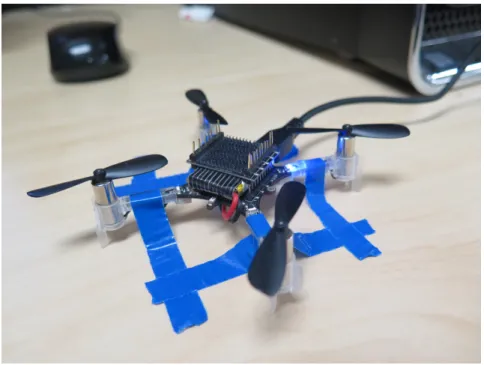
In this work, all flight tests were performed with the Crazyflie 2.0 quadrotor. For the purpose of these tests, mathematical constants inherent to the quadrotor were necessary. Most of these model parameters have already been described in [21, 19, 2, 20] as well as on internet sources. Other elements, such as the characteristics of the on-board accelerometers needed to be identified by testing. This section outlines a compilation of the information available on the Crazyflie 2.0.

3.3.1 Mass, Geometry and Inertia

The mass of the Crazyflie 2.0 with and without Vicon marker was measured with a scale in the MRASL. As for the drone’s inertial properties, a rigorous identification of the Crazyflie’s

inertia matrix was conducted in [21]. These values can be found in table 3.1 :

Table 3.1 Crazyflie 2.0 Mass, Moment of Inertia and Arm Length m (without Vicon Marker) 0.029 kg

m (with Vicon Marker) 0.032 kg Ixx = Iyy 6.410179 · 10−6kg.m2

Izz 9.80228 · 10−6kg.m2

d 39.73 · 10−3m

The layout of the Crazyflie’s propellers is in what is called the “×” configuration, meaning they are at 45 degree angle with respect to the body-frame axes. This can be seen in figure 3.2 :

Figure 3.2 Crazyflie 2.0 “×” Mode

3.3.2 Motor Characteristics

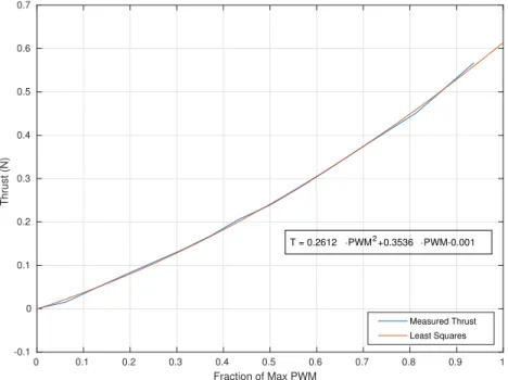
The characteristics of the thrust and moments produced have been described in several ways. This subsection presents an overview of the thrust properties that have been proposed. One interesting set of behaviours is the complete relation between input signal and output thrust.

In terms of the Crazyflie 2.0, the overall desired thrust is commanded by setting the value of a PWM2 register. This value can be between 0 − 65535, corresponding to the range between 0 and maximum thrust. Because of this high resolution, it makes numerical sense to express this value as a fraction of the maximum PWM value. Test results presented on the Crazyflie’s website3 _{were adapted to express this relation, shown in figure 3.3 :}

0 0.1 0.2 0.3 0.4 0.5 0.6 0.7 0.8 0.9 1 Fraction of Max PWM -0.1 0 0.1 0.2 0.3 0.4 0.5 0.6 0.7 Thrust (N) Measured Thrust Least Squares T = 0.2612 PWM2+0.3536 PWM-0.001

Figure 3.3 Total Thrust Produced as a Function of PWM Register Fraction

A second-order polynomial provided a good fit for this relation. Inverting it, the equivalent PWM value for a desired total force could then be calculated as in equation 3.17.

PWM = 65535 ∗−0.3536 +

q

0.35362_{+ 4 · 0.2612 · (T + 0.001)}

2 · 0.2612 (3.17)

The relation between PWM values and the resulting force coming from individual motors was also determined in [21].

In control theory, the forces and torques created by each propeller i is often modelled as being a function of the square of the angular velocity of the propeller :

2. Pulse Width Modulation

Ti = kfω2i (3.18)

τi = kτω2i (3.19)

where kf and kτ are the force and moment coefficients, respectively. Theoretical

approxima-tions of the values of kf and kτ were shown in [2] and are compiled in table 3.2 :

Table 3.2 Crazyflie 2.0 Theoretical Motor Constants kf 3.1582 · 10−10N/rpm2

kτ 7.9379 · 10−12N/rpm2

With these values and “×” configuration of figure 3.3, the total thrust and motor allocation can be expressed in terms of rotor velocities :

        f uφ uθ uψ         =             kf(ω21 + ω22+ ω32+ ω24) dkf √ 2(−ω 2 1 − ω22+ ω32+ ω42) dk_√f 2(−ω 2 1 + ω22+ ω23− ω42) kτ(−ω12+ ω22− ω32+ ω24)             (3.20)

A relation between PWM register value and propeller angular velocity was found in [21] :

ωi(rad/s) = 0.04076521 · PWM + 380.8359 (3.21)

It is important to note, however, that in real-time flight, significant firmware modifications to the Crazyflie 2.0 are needed to directly control the motors. Efforts to run a completely off-board controller that commanded rotor speeds directly were made in [19], but produced dissatisfactory results.

Finally, an empirical analysis of the z-axis torque produced by each motor was made. It was found to follow the following relation :

3.3.3 Motor Time Constant

The motor actuators were modeled to respect a first-order transfer function according to : T (s)

Tc(s)

= 1

τ s + 1 (3.23)

where Tc is the commanded force and τ was found to have a value of 45 ms after

identifica-tion. Because the implemented Kalman filter uses commanded virtual snap commands, this relation improves the accuracy of real-time estimation of the Crazyflie’s state.

3.3.4 Sensor Identification

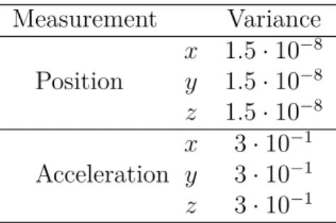
For this work, the quadrotor’s acceleration and position measurements were needed in order to complete the augmented-stated estimator presented in chapter 6. However these signals are not perfect and contain measurement noise. In order to effectively use these signals, an identification of their properties was necessary. Due to the high rate of rotation of the Crazyflie’s propellers, measurements taken by the accelerometer were prone to high levels of measurement noise. In order to quantify this noise, a simple test was performed. The drone was fastened to a stable flat surface as seen in figure 3.4 and sent a constant PWM value of 15000 for 60 seconds. A gaussian distribution was then fit to the resulting data in order to obtain a reasonable value for the white-noise variances. The results can be seen in figure 3.5.

-3 -2 -1 0 1 2 3 0 0.05 0.1 0.15 0.2 0.25 0 10 20 30 40 50 -5 0 5 -3 -2 -1 0 1 2 3 0 0.05 0.1 0.15 0.2 0.25 0.3 0.35 0 10 20 30 40 50 -5 0 5 -3 -2 -1 0 1 2 3 0 0.05 0.1 0.15 0.2 0 10 20 30 40 50 -5 0 5

Figure 3.5 Signal Identification for Acceleration Measurements

A similar procedure was performed to determine the precision of the Vicon position measu-rements. A Vicon marker was placed at the volume origin of the flight arena and its position was recorded for 60 seconds. the resulting data can be seen in figure 3.6.

These tests revealed important information about the quality of the on-board and off-board measurements. Both displayed close to gaussian behaviour, validating the assumption that the involved noise is a uniform white noise. For the accelerometer, noise variance had a range between 0.11 in the x-axis direction to 0.21 in the y-axis direction. As for the position variances, the collected data demonstrated how precise the Vicon setup was. Variances ranged from 2.43 · −9 to 1.13 · 10−8. Using these results, resulting conservative estimates of signal variances were created and compiled in table 3.3.

-5 0 5 10-4 0 0.05 0.1 0.15 0.2 0 10 20 30 40 50 60 -6 -4 -2 0 2 4 6 10 -4 -2 -1 0 1 2 10-4 0 0.05 0.1 0.15 0.2 0 10 20 30 40 50 60 -3 -2 -1 0 1 2 3 10 -4 -4 -2 0 2 4 6 10-4 0 0.05 0.1 0.15 0.2 0 10 20 30 40 50 60 -5 0 5 10 -4

Figure 3.6 Vicon Signal Properties

Table 3.3 Crazyflie 2.0 White Noise Signal Variances Measurement Variance Position x 1.5 · 10−8 y 1.5 · 10−8 z 1.5 · 10−8 Acceleration x 3 · 10−1 y 3 · 10−1 z 3 · 10−1

CHAPTER 4 EXPERIMENTAL SETUP FOR TESTING

Passing from simulation to experimental validation is a non-trivial step in the development of new quadrotor applications. This chapter aims to outline the necessary equipment and framework for the application of the control elements presented in the rest of this work. Section 4.1 outlines the specifics of ROS (Robotics Operating System), a necessary piece of software for communication between the related systems during testing. Section 4.2 presents the details of the Vicon motion capture system used for quadrotor positioning. Section 4.3 discusses the use of Matlab for off-board control and data collection. Technical details of the Crazyflie 2.0 are presented in section 4.4.

4.1 ROS

ROS is an open-source, meta-operating system commonly used in the field of robotics. It serves as the link between all of the necessary hardware used during testing. It is a complex tool, and a detailed description of ROS concepts can be found on their website1. However, there are a few fundamental elements of the ROS framework that are useful to know in order to understand how signals are sent between machines. Elements of note include :

— Nodes — Topics — Messages — Master — Packages

These elements are described in the following subsections.

4.1.1 Nodes

In the ROS network, a node is simply a process that performs computation. They can be in the form of MATLAB script, C++ code, Python code, etc. Nodes are connected to each other on the ROS network to form a graph. A typical ROS node can read (referred to as “subscribing”) information from the network, execute a calculation and then publish an output to the network. The code related to the off-board control of the drone is an example of this. First, the control node must subscribe to position, velocity, orientation and angular rate data from the network. It then computes desired forces and orientations, which are then

published to the ROS network. This information is accessed via ROS topics and is structured according to a desired message type.

4.1.2 Topics

A topic is is a named bus that allows nodes to transfer data to one another. Topics are defined on the ROS network, and have a specific structure that can contain multiple data streams. For instance, data from the on-board IMU of the Crazyflie 2.0 is received by an associated radio antenna connected to a computer on the ROS network. This data can be accessed in a terminal using the rostopic echo command :

In this example, a user is manually accessing data from the Crazyflie ROS node by subscribing to the Crazyflie topic and reading from IMU data organized in the form of a ROS message. Messages are discussed in the following subsection.

4.1.3 Messages

In ROS, a message is a data structure designed to enable the transfer of data between nodes. They are accessed by nodes via topics on the ROS network. Some examples of message types are :

— integer

— floating point — boolean — pose

Messages can store simple data, such as integer or boolean values, but can also be built to store sensor data from an IMU, or position and orientation values from a positioning system. Custom messages can also be built in order to store data structures that are not included in the default message types.

4.1.4 Master

The ROS master provides naming and registration services to the rest of the nodes in the ROS system. In other words, it allows the nodes in the ROS network to find and communicate with one another. Once nodes have established contact, they communicate directly with one another. In order to initiate the Master, the roscore command must be used :

4.1.5 Packages

In ROS, a package is a collection of files and folders that can contain nodes, libraries, datasets or any code that can be a useful independent collection of code. They are made to be easily reusable in different projects. For instance, in the case of this work, individual ROS packages were used to interface with Vicon, MATLAB and the Crazyflie 2.0 respectively. Packages can be created by manufacturers in order to enable interfacing with their products or users who want to build their own framework for robotics testing. Introductory tutorials on how to build packages and start simple ROS projects can be found on the dedicated ROS website2_.

4.1.6 Overview of ROS Network During Testing

The overall architecture of the ROS network for the tests can be seen as in figure 4.1. The controller node receives data from Vicon, Crazyflie, a joystick and a user-written “goal” node. This node interfaces with MATLAB and makes communication with the off-board controller simpler. The joystick node is used simply as a safety feature, and only sends whether a button is being pushed in order to allow the continuation of testing.

4.2 Vicon

In order to quickly and precisely measure the position of the quadrotor during testing, the MRASL relies on a Vicon motion-capture system. The system consists of a collection of 12 specialized cameras set up around the perimeter of the MRASL’s flight arena. Each of these cameras tracks a desired number of Vicon markers within its field of view (Figs 4.2 and 4.3). Combining data from all 12 cameras, high-frequency (100 Hz) estimates of position can be made to a precision of less than 1 mm. This makes Vicon a useful tool when trying to validate new types of control systems that require feedback of position and velocity.

Vicon also gives the option to track the orientation of objects in real-time. If multiple Vicon markers are attached to a rigid object, Vicon can use their displacements to estimate its rotation in 3D space. However, because of the small size of the quadrotor used in testing and the configuration of its firmware, only one marker was used and only its position was read explicitly by Vicon. Orientation estimates were read directly from inertial measurements on-board the Crazyflie.

Figure 4.1 ROS Node Architecture, from [2]

Figure 4.3 Vicon Camera Used during Testing

4.3 MATLAB

For engineering researchers, MATLAB is an indispensable tool for the simulation of new concepts. In the scope of this work, it was also useful for the implementation of controllers during testing. In order to facilitate the experiments performed, MATLAB/Simulink was used with the following add-on packages :

— ROS Package — Real-Time Pacer — Stateflow

4.3.1 ROS Package

Rather than create ROS nodes in compiled C++ or Python code, it can be practical to develop control nodes directly in Simulink. This makes changes to control structure as well as the visualization of data considerably easier for someone who is well-versed in the envi-ronment. In order to have MATLAB communicate as a node in the ROS network, the ROS add-on package must be used. After setup, this package offers blocks that can subscribe to and publish from topics on the ROS network. In the case of this work, blocks from the ROS package were used to subscribe to topics providing Vicon position data and Crazyflie sensor data. Based off of this data, control inputs could then be calculated and published to the

ROS network.

4.3.2 Real-Time Pacer

For the estimation modules used in this project, it was important for each time-step to run at a fixed frequency. By default, Simulink is intended for computer simulation and is thus designed to run as quickly as possible. This means that without management, while the state estimators used were expecting data at a frequency of 100 Hz, the actual control loop could be running much more quickly. Using the Simulink real-time package helped to solve this issue. The precision requirements for each time-step were relatively coarse (0.001 s), so the solution did not require the use of an actual real-time operating system (RTOS). Instead, the real-time package compared the simulation time with the clock of the PC being used and delayed the next time-step until the total time elapsed was 0.01 seconds. After this delay, the simulation clock was allowed to advance and new measurements, state estimates and control inputs could be calculated.

The package used was from a third party and can be found online3_.

4.3.3 Stateflow

In the case of testing, there can be multiple modes of operation and controllers. For example, a single test run for an aggressive trajectory as presented in chapter 5 begins with the motors not spinning for several seconds. The drone is then commanded to track a desired setpoint in 3D space and hover. After the drone has attained this point and reached null velocity, the drone then switches from a hover controller to a trajectory tracking controller with different architecture, followed by attitude control and finally hover control to finish the manoeuvre. Each of these controller switches has a different set of conditions in order to occur. Using conventional logic gates or user-defined functions in Simulink is possible, but inevitably creates cumbersome block diagrams that are not intuitive to read. The Simulink stateflow package enables much more elegant development of mode-switching algorithms and logic operations. More information can be found on MATLAB’s website4.

4.4 Crazyflie 2.0 Quadrotor

The drone used for testing in this work was the Crazyflie 2.0 nanoquadrotor. It is an open-source, programmable UAV that can be safely used indoors. For academic applications, it

3. http ://freesourcecode.net/matlabprojects/66903/real-time-pacer-for-simulink 4. http ://www.mathworks.com/help/stateflow/getting-started.html

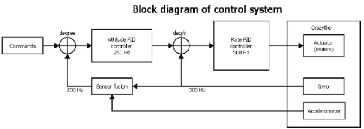
has a radio antenna called the Crazyradio PA that can plug directly into a USB port. This enables an off-board PC to send command signals to the drone at a rate of up to 100 Hz. The Crazyflie comes with a pre-programmed on-board attitude controller with the structure shown in figure 4.4 :

Figure 4.4 Crazyflie 2.0 Attitude Controller5

With the commands sent to the Crazyflie 2.0 being : — Desired roll angle φ (deg)

— Desired pitch angle θ (deg) — Desired yaw rate r (deg/sec)

— Desired overall thrust, expressed as a value between 0-65535

The on-board attitude controller receives these signals and executes 2 internal control loops. The outermost loop receives the desired roll and pitch angles and processes them at 250 Hz in a PID controller. It generates desired angular rates and sends them to an inner rate loop. This loop executes another PID controller at 500 Hz and controls for desired angular rates p, q, r. An off-board component of the attitude controller was added to the stock controller architecture in order to maintain constant yaw angle ψ throughout testing. This consisted of a PI controller that executed at 100 Hz.

The output of the on-board attitude controller is then combined with the desired overall thrust in order to calculate the desired rotor speeds :

        ω1,des ω2,des ω3,des ω4,des         =         1 −1/2 −1/2 −1 1 −1/2 1/2 1 1 1/2 1/2 −1 1 1/2 −1/2 1                 ωe+ ∆T ∆φ ∆θ ∆ψ         (4.1)

where ωe is the PWM value necessary for a stable hover, ∆T is the desired deviation from

the ωe and ∆φ, ∆θ and ∆ψ are the outputs of the PID rate-loop.

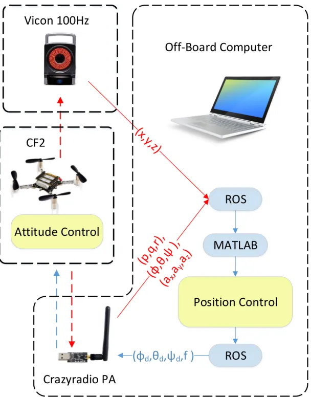
The overall organization of communication between devices in testing can be seen in figure 4.5. On-board sensor data along with Vicon position data are simultaneously sent to an off-board PC with MATLAB running. Using this information, desired angles and thrusts are calculated and sent back to the CF2 via the Crazyradio PA radio antenna.

ROS

MATLAB

ROS

Position Control

(φ

,θ

,ψ

,f )

Attitude Control

Vicon 100Hz

CF2

Off-Board Computer

Crazyradio PA

CHAPTER 5 AGGRESSIVE TRAJECTORY GENERATION

The development and execution of complex maneuvers for quadrotors has been the topic of many research papers in recent years. The ability to pass through narrow passageways at high velocities has been demonstrated with medium-sized quadrotors optimized for research purposes, notably by Mellinger, Michael and Kumar in [1]. This paper used a relatively simple approach to generate such trajectories involving the sequencing of several simple controllers to obtain a desired result. Their results showed that with a relatively simple control architecture, many possible types of complex maneuvers are possible. The technique of sequential composition was used in order to perform the passage of a quadrotor through narrow windows at varying angles as well as perching on inclined surfaces.

This chapter aims to validate such a control architecture by replicating their results in the MRASL’s flight arena at Polytechnique Montreal. Section 5.1 outlines the various controllers that were proposed in [1] and briefly discusses how they are implemented in testing. Section 5.2 describes how these controllers are sequenced in order to generate desired trajectories through windows. Finally, section 5.3 outlines the results of testing.

5.1 Control Design

The control architecture of the project consists of 3 main types of controller : — an on-board attitude controller ;

— an off-board hover controller ;

— an off-board 3D trajectory controller.

The “on-board” controllers are implemented in the firmware of the Crazyflie 2.0 and ran at either 250 Hz or 500 Hz on the device. The “off-board” controllers are managed in MAT-LAB/Simulink and executed at 100 Hz over the Crazyflie’s Crazyradio FM transmitter an-tenna. In order to achieve the desired maneuvers, these controllers are sequenced in a specific order. A detailed description of each controller follows.

5.1.1 Attitude Controller

The goal of the attitude controller controller used in [1] was to achieve a desired angle in a given settling time. It was a proportional-derivative controller with the following form :

        ω1,des ω2,des ω3,des ω4,des         =         1 −1/2 −1/2 −1 1 −1/2 1/2 1 1 1/2 1/2 −1 1 1/2 −1/2 1                 ωe+ ∆T ∆φ ∆θ ∆ψ         (5.1) ∆φ = kp,φ(φdes− φ) + kd,φ(pdes− p) (5.2) ∆θ = kp,θ(θdes− θ) + kd,θ(qdes− q) (5.3) ∆ψ = kp,ψ(ψdes− ψ) + kd,ψ(rdes− r) (5.4)

where the gains k{p,d},{φ,θ,ψ} of the controller were tuned to produce a desired time-response.

As discussed in section 4.4, the on-board attitude controller of the Crazyflie 2.0 has a similar structure. It is also augmented with integral components. This controller was tuned to have a 2% step response of time of 0.4 seconds. Validation of this controller is shown in section 5.3.

5.1.2 Hover Controller

The off-board hover controller’s goal is to attain a specified position in 3-D space within a given settling time. In order to be able to methodically find desired gains, the structure of the hover controller is slightly different from the one presented in [1] :

¨

ri,des= −kp,iri+ ki,i Z

(ri,des− ri)dt − kd,i˙ri (5.5)

With ri,des denoting the quadrotor’s x, y, and z desirced position in the world-frame and

ri the actual position. Note that this controller configuration is essentially a state-feedback

controller with integral action. Considering the non-linear system described in equation 3.3, and adding the attitude controller presented in section 5.1.1, we can produce a linearized system with the desired angles and total thrust as inputs and r, ˙r as outputs. Using ei-genstructure assignment techniques with output feedback on the measured positions and velocities, gains kp,i, ki,i and kd,i can be found numerically. For certain maneuvers, it would

be desirable to operate with an arbitrary yaw angle ψ. Linearizing (3.3), we can express the desired accelerations as a function of the desired roll, pitch and yaw angles :

¨r1,des = g(θdescos(ψdes) + φdessin(ψdes)) (5.6)

¨r2,des = g(θdessin(ψdes) − φdescos(ψdes)) (5.7)

¨r3,des =

8kFωe

m ∆T (5.8)

inverting these functions gives : φdes =

1

g(¨r1,dessin(ψdes) − ¨r2,descos(ψdes)) (5.9) θdes =

1

g(¨r1,descos(ψdes) + ¨r2,dessin(ψdes)) (5.10) ∆T =

m 8kFωe

¨

r3,des (5.11)

Depending on the phase of the maneuver, the gains of this controller are modified to fulfill specific requirements. In the first phase of each maneuver, it is important to be able to maintain a precise position in space. The first set of gains is thus designed to be the “stiffer” of the two sets, and is tuned to have a settling time of 5 seconds with an overdamped response. The hover controller is also used in the recovery stage. In this phase, the goal of the controller is just to ensure the stability of the quadrotor given potentially significant initial conditions. The second set of gains is designed to be stiff enough to prevent the quadrotor from touching the ground during recovery but not so stiff as to saturate the motors and destabilise the system.

5.1.3 3D path following

The goal of the 3D path following controller is to follow defined trajectories in 3D space. The trajectories are defined by a set of points with associated velocities. In the case of this paper, these trajectories are limited to simple line segments between points rT(i) with assigned yaw

angles ψT(i) (Fig. 5.1). At each moment, the controller evaluates which point rT(i) on the

trajectory is closest to the quadrotor and executes a specific control algorithm. In order to do this, we define ˆt, the unit tangent vector of the trajectory associated with rT(i) and desired

Figure 5.1 Line Segment Trajectory

The position error is defined as :

ep = ((rT(i) − r) · ˆn)ˆn + ((rT(i) − r) · ˆb)ˆb (5.12)

where ˆn is chosen to be a unit vector orthogonal to ˆt, and ˆb is chosen orthogonal to ˆn and ˆ

t. Here, only the normal and binormal error is considered. This ensures that the position controller will only force the quadrotor onto the line segment trajectory and not cause it to “catch up” to the next point. The velocity error is defined as :

ev = ˙rT(i) − ˙r (5.13)

The desired accelerations of the Crazyflie 2.0 can then be calculated according to the following control law :

¨

r_i,des = kp,iei,p+ kd,iei,v+ ¨ri,T(i) (5.14)

where ¨ri,T(i) corresponds to optional feed-forward acceleration elements of the trajectory.

While potentially useful in situations where the trajectory involves high accelerations, this component is set to 0 for the tests that were performed. The resulting desired overall thrusts