Equation Chapter 2 Section 1 UNIVERSITÉ DE MONTRÉAL
DEVELOPMENT OF MODELS AND A UNIFIED PLATFORM FOR MULTIPHASE LOAD FLOW ANALYSIS AND DYNAMIC STATE ESTIMATION OF LARGE DISTRIBUTION
SYSTEMS WITH SECONDARY GRIDS
BAKI EMRE CETINDAG
DÉPARTEMENT DE GÉNIE ÉLECTRIQUE ÉCOLE POLYTECHNIQUE DE MONTRÉAL
THÈSE PRÉSENTÉE EN VUE DE L’OBTENTION DU DIPLÔME DE PHILOSOPHIAE DOCTOR
(GÉNIE ÉLECTRIQUE) NOVEMBRE 2016
UNIVERSITÉ DE MONTRÉAL
ÉCOLE POLYTECHNIQUE DE MONTRÉAL
Cette thèse intitulée :
DEVELOPMENT OF MODELS AND A UNIFIED PLATFORM FOR MULTIPHASE LOAD FLOW ANALYSIS AND DYNAMIC STATE ESTIMATION OF LARGE DISTRIBUTION
SYSTEMS WITH SECONDARY GRIDS
présentée par : CETINDAG Baki Emre
en vue de l’obtention du diplôme de : Philosophiae Doctor a été dûment acceptée par le jury d’examen constitué de : M. MAHSEREDJIAN Jean, Ph. D., président
M. KOCAR Ilhan, Ph. D., membre et directeur de recherche M. KARIMI Houshang, Ph. D., membre
DEDICATION
ACKNOWLEDGEMENTS
First of all, I would like to express my deepest gratitude to my research supervisor Dr. İlhan Koçar, who is a great mentor, for his extreme patience, technical expertise, continuous guidance, opportunities he created and choosing me as a PhD student. Thank you so much for all your help. I owe gratitude to Dr. Jean Mahseredjian for the technical insight he gave, his valuable advises and providing all the help I needed. Also, I would like to thank to Dr. Ulas Karaagac for sharing his expert advice and encouragement.
I would like to thank to my father and sister for their tremendous support and constant encouragement. I especially thank my mother for the sacrifice she made the last five months by staying with me while I was writing my thesis. Without their help, I would not be able to finish this PhD.
I also thank to Dr. Akihiro Ametani, for his guidance and insightful talks.
RÉSUMÉ
Cette thèse porte sur la modélisation des différentes composantes des réseaux de distribution pour les études d'écoulement de puissance multiphasé et pour l'estimation d'état. Sans utiliser les modèles appropriés, il n’est pas possible d’obtenir des résultats précis dans l’analyse des réseaux de distribution ou des systèmes électriques en général. La thèse présente aussi un algorithme d’estimation d’état générique pour les réseaux de distribution. La performance de l’algorithme est étudiée en détail en considérant les particularités des réseaux de distribution par opposition aux réseaux de transports.
La thèse commence par la discussion sur la modélisation des régulateurs de tension pour l'écoulement de puissance en utilisant la méthode de Newton. En tenant compte des spécifications techniques de ces appareils, une nouvelle approche de modélisation est présentée en utilisant la formulation d’analyse nodale augmentée modifiée (MANA) et la méthode de Newton. Les résultats obtenus montrent que la technique proposée donne des résultats satisfaisants lorsque les réglages et les spécifications techniques des régulateurs sont considérés. Ensuite, une nouvelle méthode pour modéliser les machines asynchrones (IMs) dans l'écoulement de puissance déséquilibré est démontrée. La nouvelle approche de modélisation est encore basée sur la formulation de MANA et utilise la méthode de Newton. La nouvelle méthode peut être utilisée pour des IMs à cage simple ou double. Il permet de modéliser l’IM avec la puissance électrique, la puissance mécanique ou le couple mécanique comme contrainte. Le glissement de l'IM devient une variable d'écoulement de puissance et il est calculée itérativement. La puissance réactive est fonction de la puissance active et du glissement ou de la puissance active et de la tension de l’IM, donc il n'y a aucun besoin de fixer la puissance réactive. La solution proposée réduit le nombre d'itérations considérablement par rapport aux méthodes de solution à point fixe. La méthode présentée n'est pas actuellement disponible dans la littérature. Finalement, une approche de modélisation systématique est établie pour représenter les éoliennes (WTGs) de Type-III et Type-IV dans l'analyse d'écoulement de puissance multiphasée et déséquilibrée. Les contraintes sont écrites en fonction des composantes symétriques des courants injectés par les WTGs. Le modèle proposé pour les WTGs fonctionne bien dans des conditions déséquilibrées.
La formulation d'écoulement de puissance est ensuite reconduite pour effectuer l’estimation d’état statique des réseaux de distribution dans le domaine de phase à l’aide de la matrice Hachtel
construite à partir des équations de contraintes de MANA. En utilisant des modèles existants et des nouveaux modèles développés dans ce travail dans l’algorithme d’estimation d’état, la contribution du facteur de puissance comme pseudo-mesure sur la précision de l'estimation d’état est étudiée en posant l’hypothèse que la mesure de facteur de puissance est plus précise que la mesure de puissance. Il est remarqué que comme la grandeur du réseau augmente, l'inclusion de facteur de puissance améliore la précision de l'estimation d’état.
Finalement, différentes approches pour l'estimation d’état dynamique des réseaux de distribution sont proposées. Les méthodes sont construites en utilisant le Filtre de Kalman, les prévisions de charge et finalement la matrice Hachtel toujours construite avec la formulation MANA. Deux méthodes pour suivre le comportement dynamique des systèmes d'alimentation sont proposées. La première méthode suit l’évolution des variables d’état du réseau, ce qui est l’objectif principal des estimateurs d’état dynamique. Dans la première méthode, le point clé est de déterminer la matrice de covariance pour les prévisions. Le réglage imprécis de la matrice de covariance affecte sévèrement la performance de l'algorithme. Le réglage est obtenu en faisant de l’estimation d’état statique à plusieurs reprises afin de tenter d’obtenir le poids de chaque variable d’état. Les résultats suggèrent que l'estimateur d'état dynamique est capable de suivre avec précision l'évolution des états dans le réseau aussi longtemps que la matrice de covariance est bien réglée. La deuxième méthode peut être considérée comme une extension de l’estimateur d’état statique qui tient compte de l’évolution dynamique des mesures. Dans cette méthode, les mesures de charge sont suivies de façon indépendante et incorporés dans l’estimateur d'état après avoir été traité dans le Filtre de Kalman à l'aide du profil de charge plus ou moins précis. En absence du profil de charge, les algorithmes de lissage, comme les méthodes de lissage exponentiel, peuvent être utilisés afin d’obtenir une prédiction de mesure dans le bloc de Kalman. Cette méthode est testée sur de très grands réseaux, déséquilibrées et maillés, et une grande amélioration est atteinte dans les résultats par rapport à l'estimateur statique. Grâce à la formulation de Newton, la technique proposée est capable d’analyser de très grands réseaux de distribution, avec plus de vingt mille nœuds, en 3 ou 4 itérations.
Les algorithmes développés fonctionnent bien sur les grands réseaux. Au meilleur de la connaissance de l'auteur, cette thèse est la première à démontrer une solution pour l'estimation d'état de très grands réseaux de distribution avec des topologies maillées du côté basse tension ou secondaire (tels que ceux de New York, Chicago et Toronto).
ABSTRACT
This thesis is on the modeling of various components of distribution systems for multiphase load flow studies and state estimation. Without employing proper models, it is not feasible to obtain accurate results in the analysis of distribution networks or power systems in general. The thesis presents also a generic state estimation solver for distribution networks. The performance of the solver is investigated in detail considering the particularities of distribution networks as opposed to transmission grids.
The thesis starts by discussing the modeling of step voltage regulators for load flow using Newton’s method. By taking into account the technical specifications of these devices, a new modeling approach is presented within the modified augmented nodal analysis (MANA) formulation and Newton’s method. The results obtained show that the proposed technique gives satisfactory results as far as the settings and technical specifications of the regulators are concerned. Afterwards, a new method to model Induction Machines (IMs) in unbalanced load-flow calculations is demonstrated. The new modeling approach is again based on the MANA formulation and employs Newton’s method. The new method can be used for single and double cage IMs. It allows modeling the IM with electrical power input, mechanical power or mechanical torque output. The slip of the IM becomes a load-flow variable computed iteratively. The reactive power is a function of real power constraint and slip or voltage solution of the IM, therefore there is no need to fix the reactive power input. The proposed solution reduces the number of iterations radically as compared to fixed-point solution methods. The presented formulation is not currently available in the literature. Finally, a systematic modeling approach is established to represent Type-IV and Type-III wind turbine generators (WTGs) in multiphase and unbalanced load flow analysis. The proposed approach integrates the constraints based on the sequence components of the injected currents from WTGs. The proposed model for WTGs performs well under unbalanced conditions.
The load flow formulation is then extended to perform static state estimation of distribution networks in phase frame using Hachtel matrix built with MANA constraint equations. By using the existing and new models developed in this work, the contribution of the load power factor pseudo-measurement on the accuracy of state estimation is investigated putting forward the hypothesis that the power factor measurement is more accurate than the power measurement. It is observed that as
the size of the network increases the inclusion of power factor improves the accuracy of state estimation.
Finally, different approaches for the dynamic state estimation of distribution networks are proposed. The formulations are built using Kalman Filter, load forecasting and Hachtel matrix built with MANA formulation. Two methods tracking the dynamic behavior of power systems are proposed. The first method tracks the change of the state variables of the network, which is the main objective of the dynamic state estimators. In the first method, the key point is to determine the covariance matrix for the forecasts. Inaccurate tuning of the covariance matrix, which means poorly defined diagonal elements, affects the performance of the algorithm severely. The tuning is achieved by performing static state estimation repeatedly in order to attempt to obtain the weight of each state variable. The results suggest that the dynamic state estimator is able to accurately track the evolution of states in the network as long as the covariance matrix is well tuned. The second method can be considered as an extension to the static state estimator that considers the dynamic evolution of measurements. In this method, the load measurements are tracked independently and incorporated into state estimator after being processed in Kalman Filter using the load pattern. In the absence of load pattern, smoothing algorithms, such as exponential smoothing methods, can be used to obtain a prediction of measurements in the Kalman block. This method is tested on very large, unbalanced and meshed networks, and a great improvement is attained in the results compared to the static estimator. Thanks to its Newton formulation, the proposed technique is capable of analyzing very large distributing networks with more than twenty thousand nodes within 3 or 4 iterations.
The developed algorithms scale up and work well on large networks. To the best of author’s knowledge, this thesis demonstrates a solution for the state estimation of extremely large scale distribution networks with secondary grid details (such as the ones in New York, Chicago and Toronto) for the first time.
TABLE OF CONTENTS
DEDICATION ... III ACKNOWLEDGEMENTS ... IV RÉSUMÉ ... V ABSTRACT ... VII TABLE OF CONTENTS ... IX LIST OF TABLES ... XIV LIST OF FIGURES ... XVI LIST OF SYMBOLS AND ABBREVIATIONS ... XXI LIST OF APPENDICES ... XXVIINTRODUCTION ... 1
MANA LOAD FLOW ... 4
2.1 The Steady-State Form of MANA ... 4
2.1.1 The Formation of
Y
n andI
n ... 52.1.2 The Formation of
V
r andV
b ... 72.1.3 The Formation of
D
r ... 82.1.4 The Formation of
S
r andS
d ... 92.2 The Load Flow Analysis in MANA ... 10
2.2.1 The Linear Constraints ... 13
2.2.1.1 The Kirchhoff’s Current Law ... 13
2.2.1.2 The Ideal Voltage Source Constraint ... 13
2.2.1.3 The Branch Dependent Device Constraint ... 14
2.2.2 The Load Constraints ... 14
2.2.2.1 The Jacobian Terms of the Real Power Constraint ... 17
2.2.2.2 The Jacobian Terms of the Reactive Power Constraint ... 17
2.2.3 The Conventional Generator Constraints ... 18
2.2.3.1 The Generator Current (Linear) Constraint ... 21
2.2.3.2 The Total Injected Real Power Constraint ... 21
2.2.3.3 The Total Injected Reactive Power Constraint ... 23
2.2.3.4 The Magnitude Constraint Defined on Phase Voltage ... 24
2.2.3.5 The Magnitude Constraint Defined on Positive Sequence Voltage ... 25
2.2.3.6 The Phasor Constraint Defined on the Positive Sequence Voltage Phasor ... 26
2.2.4 Convergence Criteria ... 27
2.3 Summary ... 28
STEP VOLTAGE REGULATORS ... 29
3.1 The Voltage Regulator Model ... 29
3.2 The Constraints and Jacobian Terms ... 35
3.2.1 Voltage Constraints ... 35
3.2.2 Current constraints ... 36
3.2.3 Voltage Magnitude Constraint at the Load Center ... 36
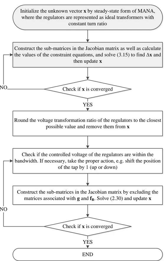
3.3 Solution Algorithm and Considerations ... 37
3.3.1 Load Flow with “
g
” Being Variable ... 383.3.2 Load Flow After Fixing “
g
” ... 383.4 Study Cases ... 41
3.4.1 Study Case-1: Remote Location Voltage Control ... 41
3.5 Summary ... 48
ASYNCHRONOUS MACHINES ... 49
4.1 Induction Machine Model ... 49
4.2 The Constraints and Jacobian Terms ... 53
4.2.1 Contributions to Current Injection Constraint ... 54
4.2.2 Electrical Power Constraint ... 56
4.3 Study Cases ... 57
4.3.1 Study Case-1: Induction Machine Test Case ... 57
4.3.2 Study Case-2: Induction Machine Test Case for the 34-Bus Test Feeder ... 62
4.4 Summary ... 68
ELECTRONICALLY COUPLED GENERATORS ... 69
5.1 The Electronically Coupled Generator Model ... 69
5.1.1 Type-III Wind Turbine Model ... 69
5.1.2 Type-IV Wind Turbine Model ... 70
5.1.3 The Proposed Model ... 71
5.2 The Constraints and Jacobian Terms ... 72
5.2.1 The Negative Sequence Constraints ... 74
5.2.2 The Zero Sequence Constraints ... 76
5.2.3 The Positive Sequence Constraints ... 78
5.2.3.1 The Positive Sequence Real Power ... 78
5.2.3.2 The Positive Sequence Reactive Power ... 79
5.2.3.3 The Magnitude of the Positive Sequence Voltage ... 80
5.3 Study Cases ... 81
5.3.2 Study Case-2: IEEE 39 Bus Test Case ... 84
5.3.3 Study Case-3: The Comprehensive Test Case ... 87
5.4 Summary ... 95
MULTIPHASE STATIC STATE ESTIMATION AND THE EFFECT OF THE LOAD POWER FACTOR PSEUDOMEASUREMENT ON ITS ACCURACY ... 96
6.1 General Formulation ... 97
6.2 State Estimation Algorithm in MANA ... 100
6.2.1 Covariance Matrix
R
cov ... 1006.2.2 Network Constraints ... 101
6.2.3 Measurement Equations ... 102
6.2.3.1 Node Voltage Measurement ... 103
6.2.3.2 Branch Current Measurement ... 103
6.2.3.3 Branch Power Measurement ... 104
6.2.3.4 Phasor Measurement Unit (PMU) ... 105
6.3 The Load Power Factor ... 105
6.4 Study Cases ... 107
6.4.1 Study Case-1: IEEE 13 Bus Network: ... 108
6.4.2 Study Case-2: IEEE 34 Bus Test Case ... 109
6.4.3 Study Case-3: IEEE 342 Node Distribution Network ... 111
6.4.4 Study Case-4: Large Scale Distribution Network ... 114
6.5 Summary ... 116
DYNAMIC STATE ESTIMATION IN MANA ... 117
7.1 State Forecasting ... 118
7.1.2 Adaptive Response Rate Single Exponential Smoothing (ARRSES) ... 118
7.1.3 Double Exponential Smoothing: Holt’s Two Parameter Method (DES) ... 119
7.2 Dynamic Mathematical Model ... 120
7.2.1 Parameter Identification for SES ... 120
7.2.2 Parameter Identification for ARRSES ... 120
7.2.3 Parameter Identification for DES ... 121
7.3 Extended Kalman Filter Algorithm ... 122
7.4 Objective Function of Dynamic State Estimation ... 124
7.5 Proposed Method I: Hachtel Based Dynamic State Estimator ... 125
7.6 Proposed Method II: Semi-Dynamic State Estimator ... 127
7.7 Measurement Test ... 129
7.8 Study Cases ... 130
7.8.1 Study Case-1: IEEE 342 Node Distribution Network ... 131
7.8.1.1 Scenario-1: ... 131
7.8.1.2 Scenario-2: ... 135
7.8.2 Study Case-2: IEEE 34 Bus Test Case ... 139
7.8.3 Study Case-3: Real Distribution Network ... 142
7.9 Summary ... 147
CONCLUSION AND RECOMMENDATIONS ... 148
BIBLIOGRAPHY ... 151
LIST OF TABLES
Table 3.1: Regulator Relay data ... 42
Table 3.2: Tap Positions ... 43
Table 3.3: Tap Positions ... 47
Table 4.1: Induction Motor Solution ... 59
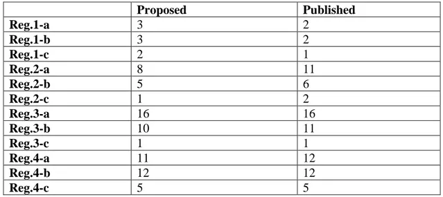
Table 4.2: Slip Values ... 64
Table 4.3: Generator Solution ... 64
Table 5.1: The Generator Parameters ... 82
Table 5.2: The Generator Sequence Currents ... 84
Table 5.3: The Generator Constraints ... 86
Table 5.4: The IM Generator Parameters ... 88
Table 5.5: The Transformer Parameters ... 88
Table 5.6: The IM Groups ... 88
Table 5.7: The ECG Parameters ... 89
Table 5.8: The Resultant Slip Values for the IMs ... 90
Table 5.9: The Resultant Tap Positions ... 91
Table 5.10: The Resultant Controlled Voltages ... 91
Table 6.1: Standard Deviation of the Measurements ... 109
Table 6.2: Standard Deviation of the Measurements ... 110
Table 6.3: Network Parameters ... 114
Table 7.1: Evaluation of Performance ... 133
Table 7.2: Evaluation of Performance ... 136
LIST OF FIGURES
Figure 2.1: RLC Impedance Connected between k and Ground ... 6
Figure 2.2: Ideal Voltage Source ... 7
Figure 2.3: Hybrid Model of a Two Port Network ... 8
Figure 2.4: (a) Open Switch (b) Closed Switch ... 9
Figure 2.5: Generic Load Model ... 14
Figure 2.6: Generic Generator Model ... 18
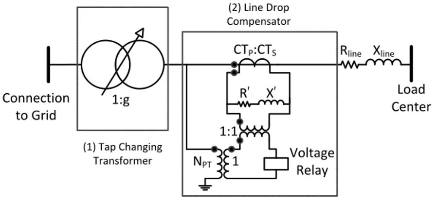
Figure 3.1: Voltage Regulator Circuit Diagram ... 29
Figure 3.2: Simplified Regulator Model ... 32
Figure 3.3: Simplified Regulator Circuit ... 33
Figure 3.4: Flowchart of the Load Flow with the insertion of Regulators ... 40
Figure 3.5: IEEE 13 Node Test Feeder ... 41
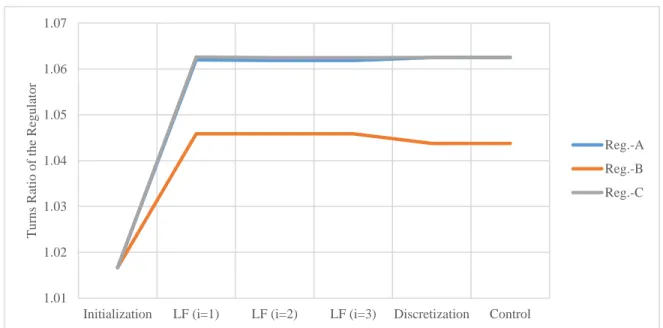
Figure 3.6: The evolution of the voltage transformation ratio of the regulators ... 43
Figure 3.7: The Voltage Profile of the Network ... 44
Figure 3.8: The Voltage on the Relay ... 44
Figure 3.9: IEEE 8500-Node Test Feeder ... 45
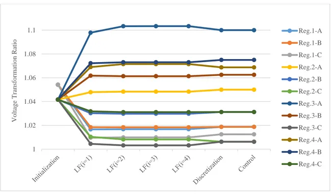
Figure 3.10: The Evolution of the Voltage Transformation Ratio of the Regulators ... 46
Figure 3.11: Magnitudes of the Voltages at the Controlled Nodes ... 48
Figure 4.1: Single Cage Squirrel Machine Model ... 49
Figure 4.2: Double Cage Squirrel Machine Model ... 50
Figure 4.3: The Direction of the Machine Currents ... 51
Figure 4.4: Network Schematic for the Study Case-1 ... 58
Figure 4.6: Voltage Magnitude ... 59
Figure 4.7: Voltage Angle ... 60
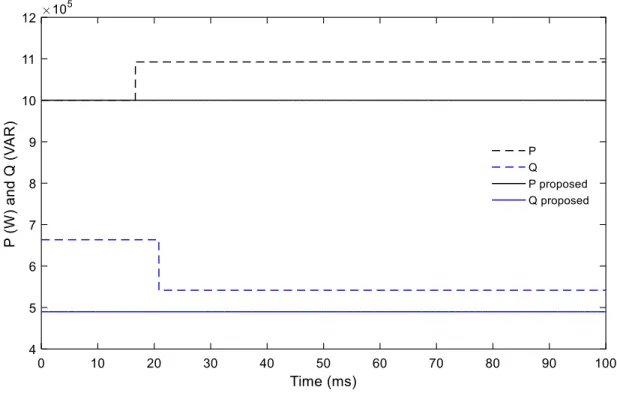
Figure 4.8: PQ input of IM from Load-Flow to Time-Domain ... 61
Figure 4.9: PQ input initialization of IM, unbalanced 4-BUS ... 62
Figure 4.10: Network Schematic for the Study Case-2 ... 63
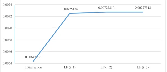
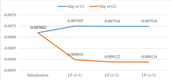
Figure 4.11: Evolution of the Slip of the IM ... 63
Figure 4.12: Voltage Magnitude ... 65
Figure 4.13: Voltage Angle ... 65
Figure 4.14: G1 IM-G1 Currents, Phases A, B and C ... 66
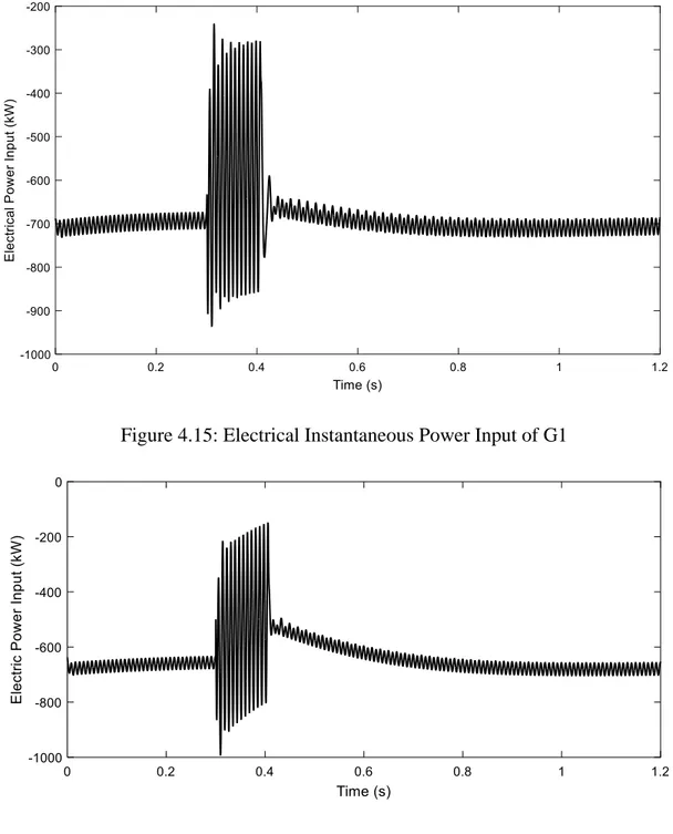
Figure 4.15: Electrical Instantaneous Power Input of G1 ... 67
Figure 4.16: Electrical Instantaneous Power Input of G2 ... 67
Figure 5.1: Circuit Diagram of a Single DFIG ... 70
Figure 5.2: Circuit Diagram of a Type-IV WTG ... 71
Figure 5.3: Current Source Representation of ECGs ... 71
Figure 5.4: IEEE 34 Bus with a Generator Unit ... 82
Figure 5.5: Voltage Profile of the Network (Proposed Model) ... 83
Figure 5.6: Voltage Profile of the Network (Classical Model) ... 84
Figure 5.7: Network Schematic of IEEE 39 Bus Test Case ... 85
Figure 5.8: Voltage Profile of the Network ... 87
Figure 5.9: Induction Machine Group ... 87
Figure 5.10: Secondary LV Grid with Single Phase Generator ... 89
Figure 5.11: Iteration vs. Slip for All Groups (IM-1) ... 92
Figure 5.12: Iteration vs. Slip for All Groups (IM-2) ... 92
Figure 5.14: Iteration vs. Slip for All Groups (IM-4) ... 93
Figure 5.15: Iteration vs. Slip for All Groups (IM-5) ... 94
Figure 5.16: Iteration vs. Turn Ratio (Solver-1) ... 94
Figure 5.17: Iteration vs. Turn Ratio (Solver-2) ... 95
Figure 6.1: Probability Distribution Function of a White Signal ... 100
Figure 6.2: Closed Switch between k and m ... 104
Figure 6.3: Load Power in Rectangular Form ... 105
Figure 6.4: The Limits for the Load Angle ... 106
Figure 6.5: Load Power in Rectangular Form ... 107
Figure 6.6: IEEE 13 Bus Test Feeder with the Positions of Measurements ... 108
Figure 6.7: Comparison of Method-I and Method-II ... 109
Figure 6.8: IEEE 34 Bus Test Network with Measurements ... 110
Figure 6.9: Comparison of Method-I and Method-II for the Study Case-II ... 111
Figure 6.10: Comparison of Method-I and Method-II for the Study Case-II ... 111
Figure 6.11: Single Line Diagram of IEEE 342 Node Distribution Network ... 112
Figure 6.12: Comparison of Method-I and Method-II ... 113
Figure 6.13: Worst Case Scenario for the Study Case-3 ... 114
Figure 6.14: Comparison of Mean Error for Method-I and II ... 115
Figure 6.15: Comparison of Worst Case Scenario for Method-I and II ... 116
Figure 7.1: The Flow Chart of Iterated Extended Kalman Filter ... 123
Figure 7.2: The Overall Algorithm of Iterated Extended Kalman Filter ... 124
Figure 7.3: Hachtel based Dynamic State Estimator ... 126
Figure 7.4: Semi-Dynamic State Estimation ... 129
Figure 7.6: Voltage Magnitude at S188b ... 133
Figure 7.7: Voltage Magnitude at P109a ... 134
Figure 7.8: Voltage Magnitude at S205c ... 134
Figure 7.9: Voltage Magnitude at P3b ... 135
Figure 7.10: Load Profile for the Scenario-II ... 135
Figure 7.11: Voltage Magnitude at S188c ... 136
Figure 7.12: Voltage Magnitude at P109b ... 137
Figure 7.13: Voltage Magnitude at S196a ... 137
Figure 7.14: Voltage Magnitude at S196a ... 138
Figure 7.15: Measurement Test ... 138
Figure 7.16: Morning Load Pattern ... 139
Figure 7.17: Voltage Magnitude at 816c ... 140
Figure 7.18: Voltage Magnitude at 816c ... 140
Figure 7.19: Voltage Magnitude at 856b ... 141
Figure 7.20: Voltage Magnitude at 890c ... 141
Figure 7.21: Single Line Diagram of the Primary Distribution Network ... 142
Figure 7.22: Voltage Magnitude at 12783c ... 143
Figure 7.23: Voltage Magnitude at 13091a ... 144
Figure 7.24: Voltage Magnitude at 13774b ... 144
Figure 7.25: Voltage Magnitude at V7992a ... 144
Figure 7.26: Voltage Magnitude at V1474b ... 145
Figure 7.27: Voltage Magnitude at 24M74colonM41745b ... 145
Figure 7.28: Voltage Magnitude at 12977c ... 145
Figure 7.30: Voltage Magnitude at 24M89colonM48458b ... 146 Figure 7.31: Voltage Magnitude at 24M98colonM13634b ... 146 Figure 7.32: Voltage Magnitude at 24M91colonM48520c ... 147
LIST OF SYMBOLS AND ABBREVIATIONS
Absolute Value Operator
A System Matrix of a Network in Steady-State
f
A Fortescue Transformation Matrix
IL
A Adjacency Sub-Matrix of Load Currents
IG
A Adjacency Sub-Matrix of Generator Currents
SM
A Jacobian Sub-Matrix of Kirchhoff’s Current Law w.r.t IM Slips
G
B Jacobian Sub-Matrix of Generator Current Constraints w.r.t Generator Currents ARRSES Adaptive Rate Response Single Exponential Smoothing
c Constraint Equations
L
C Jacobian Sub-Matrix of Load Constraints w.r.t Node Voltages
G
C Jacobian Sub-Matrix of Generator Constraints w.r.t Node Voltages
RV
C Jacobian Sub-Matrix of Regulator Constraints w.r.t Node Voltages
RI
C Jacobian Sub-Matrix of Regulator Constraints w.r.t Branch-Dependent Currents
RG
C Jacobian Sub-Matrix of Regulator Constraints w.r.t Turns Ratio
M
C Jacobian Sub-Matrix of IM Constraints w.r.t Node Voltages
SM
C Jacobian Sub-Matrix of IM Constraints w.r.t IM Slips
CG
C Jacobian Sub-Matrix of ECG Constraints w.r.t Node Voltages
P
CT Primary Current Rating of a Current Transformer
S
CT Secondary Current Rating of a Current Transformer
L
G
D Jacobian Sub-Matrix of Generator Constraints w.r.t Generator Currents
r
D Dependency Sub-Matrix of Branch Dependent Devices
CG
D Jacobian Sub-Matrix of ECG Constraints w.r.t ECG Currents DES Double Exponential Smoothing
DSE Dynamic State Estimation
G
E Vector of Internal Generator Positive Sequence Voltages ECG Electronically Coupled Generators
EKF Extended Kalman Filter
F State Transition Matrix
n
f Vector of Kirchhoff’s Current Law Constraints
v
f Vector of Voltage Source Constraints
d
f Vector of Branch-Dependent Device Constraints
s
f Vector of Switch Constraints
E
f Vector of Generator Current Constraints
L
f Vector of Load Constraints
G
f Vector of Generator Constraints
CG
f Vector of ECG Constraints
E
f Vector of Generator Current Constraints
R
f Vector of Regulator Constraints
M
f Vector of IM Constraints
g Vector of Voltage Transformation Ratio
v
I Vector of Voltage Source Currents
d
I Vector of Branch-Dependent Devices Currents
s
I Vector of Switch Currents
n
I Vector of Injected Currents at Each Node
L
I Vector of Load Currents
G
I Vector of Generator Currents
CG
I Vector of ECG Currents
IM Induction Machine
IEKF Iterated Extended Kalman Filter GSC Grid Side Converter
J Jacobian Matrix
c
J Jacobian Matrix of Constraints
h
J Jacobian Matrix of Measurements
K Kalman Gain Matrix
KF Kalman filter
LF Load Flow
MANA Modified Augmented Nodal Analysis MSC Machine Side Converter
PT
N Turns Ratio of a Voltage Transformer
P Real Power
R Compensator Network Resistance Setting
line
cov
R Covariance Matrix of Measurements Q Covariance Matrix of Process Error
Q Reactive Power
RLC Resistance-Inductance-Capacitance RSC Rotor Side Converter
M
s Vector of IM Slips
r
S Adjacency Sub-Matrix of Ideal Switches in Closed Position
d
S Adjacency Sub-Matrix of Ideal Switches in Open Position SES Single Exponential Smoothing
SSE Static State Estimation
n
V Vector of Node Voltages
r
V Adjacency Matrix of Ideal Voltage Sources
b
V Vector of (Voltage) Source Voltages
n
Y Admittance Matrix
G
Y Jacobian Sub-Matrix of Generator Current Constraints w.r.t Node Voltages
GE
Y Jacobian Sub-Matrix of Generator Current Constraints w.r.t Internal Voltages
x State Vector
x Forecasted State Vector ˆx True State Vector
X Compensator Network Reactance Setting
line
X Feeder Reactance
LIST OF APPENDICES
APPENDIX-A: PARAMETERS OF INDUCTION MACHINE TEST CASE………156 APPENDIX-B: MACHINE PARAMETERS OF INDUCTION MACHINE TEST CASE FOR IEEE 34 NODE TEST FEEDER………...158
INTRODUCTION
The smart grid initiatives and increasingly stringent conditions of reliability, sustainability, cost and environmental impacts drive major transformations in distribution networks, not only in terms of infrastructure and circuit topology but also in terms of operation philosophy. In addition to the existing secondary grid networks found in certain urban distribution systems, microgrid integration is becoming more and more common at the distribution level. There are many distribution utilities which are required to operate their networks starting from the subtransmission level. Moreover, the increased integration of distributed generation units in distribution networks has introduced the concept of Active Distribution Networks (ADNs) in power systems. Due to its higher dynamics compared to the conventional distribution networks, an ADN is characterized by the need for voltage control, unique protection schemes, frequency and reactive power control. Therefore, the real-time control of ADNs is an important task and requires reliable state estimation algorithms which need to be fast, at the same time accurate enough to correctly model the distribution system components.
In this thesis, multiphase load flow modeling of various components in modern distribution networks is presented as a first step, since without proper models, it is not feasible to obtain valid results following the analysis of the circuits. Afterwards, dynamic and static state estimation of distribution networks are investigated.
Chapter-2 is the review of the Modified Augmented Nodal Analysis (MANA) approach [1-3] and its applications in steady-state and the load-flow [4, 5] analyses. The linear form of MANA provides the steady-state phasor solution and is obtained by representing the network components with their linear equivalents. The Jacobian form of MANA is used as the basis for performing load flow analysis by transforming the system of equations into Jacobian form and by extending it with nonlinear constraint equations for various components such as generators and loads. The common device models that are already available in the literature are provided here in a compact form both for steady state and load flow analyses using a systematic notation. The objective here is to set the stage for the development of new models and to get the reader familiarize with the methodology and the state-of-the-art in this field. The expandable matrix structure of MANA [1-3]allows the addition of both linear and nonlinear devices in block forms. It has a modular formulation such that addition of a new device does not require modifying the previously defined blocks.
In Chapter-3, the step voltage regulators which are critical for maintaining voltage profile on long distribution feeders are discussed. They are the primary equipment used in Volt/Var optimization. First, their operation and physical structure are explained in detail. Subsequently, the equations that form the constraints for load flow formulation are presented. As is well known, the primary functionality of a voltage regulator is to adjust the voltage of the controlled node given the voltage settings and limits. In the proposed technique, the magnitude of the controlled voltage is therefore the constraint equation.
Chapter-4 describes the integration of the induction machines into load flow formulation. Accurate modelling of the distributed generation units in load-flow solvers is an important criterion when evaluating the performance of the algorithms. The asynchronous induction machines (IM) constitute an important part of a distribution network, and are often modeled as constant PQ devices in the load-flow solution, but there is no direct relation between real and reactive powers of the IM in reality. In the proposed model, MANA approach has been expanded to account for the IMs by considering the slip of each IM as an unknown variable which is to be calculated iteratively. The constraint is the active power and there is no fixation of reactive power. Although the IM has been modeled with active power constraint only in the literature, the published methods rely on fixed point techniques and treat the IM in separate while performing load flow solution. This requires huge number of iterations and the convergence is not guaranteed due to fixed point approach. The integration of IM into Jacobian and the use of a full Newton method are presented for the first time in this work.
In Chapter-5, the electronically coupled generators (ECGs) or distributed energy resources (DERs) are investigated and modeled using MANA load flow formulation. The existing generator model which is explained in the Chapter-2 is not sufficiently accurate. In the classical generator model, a generator is represented by a voltage source behind a Thevenin impedance, which is also the widely used model in the literature [6-14]. On the other hand, the utility scale solar parks or wind parks either control the terminal voltage or reactive power injection. They can have decoupled reactive and active power controls and the grid side converters adjust the power by adjusting the active and reactive current references. Therefore, in multiphase load flow solution under unbalanced conditions, balanced voltage source behind an impedance model, used to represent traditional generators cannot truly represent the full behavior of ECGs. In [15], a technique to represent electronically coupled devices as current injections is presented where the sequence components
are used in constraint equations. In [16], a method based on branch current injection is proposed for radial systems. In [17], the wind parks have been modelled as an impedance as a function of slip assuming it as an induction machine but the most recent wind parks are either Type-III or Type-IV [18] and thus power electronics must be considered in the models. In the proposed model, a current source based model in MANA is presented by taking into account the control circuitry. This is an important contribution since this approach allows integrating different controls into load flow solution in a simple and robust manner.
Chapter-6 investigates the effect of the load power factor in the state estimation and presents a static state estimation [19, 20] algorithm based on the Hachtel formulation [21] by expanding MANA approach for various measurement equations. The method presented is well suited to meshed networks. This is the main advantage over the existing state estimation solvers for distribution networks [22-29] which are mostly designed for radial systems. In this chapter, it is aimed to show when the information related to the power factor available, the state estimation gives better results for distribution networks.
In Chapter-7, the dynamic behavior of the networks is studied and a new approach for the dynamic state estimation of distribution networks is proposed. Unlike its static counterpart described in Chapter-6, the dynamic state estimator also employs the previous estimates of the network to generate virtual measurements. There are numerous advantages of the dynamic state estimation over the static one. It allows longer decision time to the operator of the system, since security assessment, economic dispatching (subtransmission level), etc. can be realized earlier. Most of the dynamic state estimators [30, 31] are based on Kalman filtering [32]. In this thesis, an alternative approach is proposed within the context of the weighted least squares (WLS) method. In this chapter, the Kalman type estimators are reviewed before developing the proposed method which is an extension to the static state estimator obtained by considering the dynamic evolution of measurements. In this method, the load measurements are tracked independently and incorporated into state estimator after being processed in Kalman Filter using the load pattern. In the absence of load pattern, smoothing algorithms, such as exponential smoothing methods are suggested to obtain a prediction of measurements in the Kalman block. This method is tested on very large, unbalanced and meshed networks, and a great improvement is accomplished in the results when compared to the static estimator.
MANA LOAD FLOW
2.1 The Steady-State Form of MANA
The MANA formulation originates from the classical nodal analysis (NA). Its main advantage is to allow independent modeling of devices. The general MANA formulation for a linear network in steady-state has the following form [3]:
n c c c n n r d vd vs v b d b r dv d ds s d r sv sd d x b A Y V D S V I V V D S I V = I d D D D S I s S S S S (1.1)
The general formulation in (1.1) is the most generic form and contains all device equations. In this thesis, the simplified version of (1.1) is used instead:
T T T n r r r n n r v b r d s r d x b A Y V D S V I V 0 0 0 I V D 0 0 0 I 0 I 0 S 0 0 S (1.2)
The equation (1.2), which will be referred as the steady-state form from this point onward is written in the complex domain and is used to find the unknowns in phasor form. The subscript (T) indicates the transpose of a matrix or vector. Throughout this document, the arrow on top of a vector or matrix term indicates that the term can be complex and a transformation into a form of real vectors or matrices is required. For any complex matrix C, the real form is given by;
Re Im Im Re C C C C C (1.3)Similarly, the real form of a complex valued vector v is written in a similar way:
Re Im v v v (1.4)where Re and Im are the real and imaginary part operators, respectively.
In the formulation above, the system matrix A on the left hand-side has the following components:
n
Y : The admittance matrix of the linear network
r
V : The adjacency matrix of the ideal voltage sources
r
D : The voltage dependency matrix of the branch-dependent devices
r
S : The adjacency matrix of the ideal switches (closed)
d
S : The adjacency matrix of the ideal switches (open)
The unknown vector x is composed of the following components:
n
V : The vector containing the node voltage phasors
v
I : The vector containing the current phasors through each ideal voltage source
d
I : The vector containing the current phasors of the branch dependent devices
s
I : The vector containing the current phasors of all switches
The known quantities vector b on the right hand side is formed by the following components:
n
I : The vector of the injected current phasors at each node
b
V : The vector of the voltage source phasors The system in (1.2) can be solved by direct methods.
2.1.1 The Formation of
Y
nand
I
nThe formation of Y is straightforward. Now, assume an impedance indexed with n p is connected
between the nodes k and ground as shown in Figure 2.1, and Zp Rp jXp in where R and p p
p p p
Z R jX
k
Figure 2.1: RLC Impedance Connected between k and Ground Its contribution to Y can be expressed with an update equation as follows; n
,
, new old p k k k k Y n n Y Y (1.5) where Yp Zp1If that impedance is connected between the nodes k and m instead, three other parameters need to be updated as well:
, , , , , , new old p new old p new old p m m m m Y m k m k Y k m k m Y n n n n n n Y Y Y Y Y Y (1.6)If the component to be included in Y is a three phase element such as a 3 phase line, (1.5) and n (1.6) are still valid. In that case, Yp becomes a 3 by 3 matrix, and m and k represent the 3 by 1
node vector.
In steady-state form of MANA, the following elements contribute to the construction of Y : n Lines and cables which are represented with PI-model
PQ loads with their nominal impedance Internal impedance of the transformers
Induction machines with Steinmetz circuit representation Any combination of RLC elements
The phasors of the current sources are represented in I . Let a current source with the phasor n
p p
I be connected at the node k. If the direction is chosen as ‘into the node’; then,
k Ip pn
If there are several current sources are connected to the same node, the sum of current injections must be considered.
2.1.2 The Formation of
V
rand
V
bAn ideal voltage source keeps the voltage and the angle of the nodes constant where it is connected. Different configurations of ideal voltage sources can be realized within MANA formulation [5].
AC1 AC2
k
m
n
Figure 2.2: Ideal Voltage Source
In Figure 2.2, the first voltage source AC1 is connected between the nodes k and m; while the second voltage source AC2 is connected between the node n and the ground. Let VAC1AC1 and
2 2
AC AC
V denote the phasors of the sources AC1 and AC2 respectively. Then, the formulations of V and r V become [3]: b
2 2 1 1 1, 1 2, 1 1, 1 2 1 AC AC AC AC p ka p n p kb p V p V r r r b b V V V V V (1.8)where p1 and p2 are the indices for AC1 and AC2.
In steady-state form of MANA, the following elements are represented in V : r
Single/Three phase ideal voltage sources
Slack generators can also be included in V as their terminal voltage phasor is a known r quantity.
2.1.3 The Formation of
D
rThe branch related components refer to the elements whose output (or behavior) depends on the state of the system. A single phase ideal transformer can be modeled as a two port device and its hybrid model is demonstrated in Figure 2.3. The matrix containing the hybrid parameters for this model can be expressed as follows [5]:
11 12 2 2 21 22 1 1 h h V I h h I V (1.9) h21 I2 k1 k2 h12 V1
+
-m2 V1 I2 m1 I1 V2
Figure 2.3: Hybrid Model of a Two Port Network An ideal transformer can be defined by two equations:
2 2 1 1 V N g N V (1.10) 1 1 2 2 1 2 N I N I or I gI (1.11)
where N and 1 N are the number of turns, and 2 g is the turns ratio of the transformer. Then, the hybrid parameters of (1.9) become [5]:
1 2 1 2 0
m m k k
V V gV gV (1.12)
, 1 , 2 , 1 1 , 2 1 p k g p k g p m p m r r r r D D D D (1.13)The elements that can be modeled using D are as follows: r
Three phase transformers can be modeled as a combination of single phase units Autotransformers
Regulators
2.1.4 The Formation of
S
rand
S
dThe switches can be represented in MANA without representing them in Y as zero and/or infinite n
impedance. Consider the two switches in Figure 2.4. The switch SW1, which connected between the nodes k1 and m1, is open and the switch SW2, which is connected between the nodes k2 and
2
m , is closed. R is represents the switch resistance of the non-ideal switches which is quite low. sw
SW1 k1 m1 SW2 k2 m2 sw R sw R
Figure 2.4: (a) Open Switch (b) Closed Switch
Let p denote the index of SW1 and q denote the one of SW2. Then, pth element of I gives s
the unknown current phasor of SW1 and qth element of I gives the unknown current phasor of s
2 SW .
1 2 SW SW p I q I s s I I (1.14)An open switch does not allow any current to pass on it. Thus, ISW1 must be set to zero. The corresponding entry of S is given by the formula [5]: d
p p ,
1d
S (1.15)
When the switch is in closed position, the equation which describes its function [5]:
2 2 2 k m SW sw V V I R (1.16)
Thus, the corresponding entries of S and r S are given as [5]: d
1 , 2 1 , 2 , 1 sw sw q k R q m R q q r r d S S S (1.17)2.2 The Load Flow Analysis in MANA
In the previous section, the solution of a time invariant network is presented where all elements can be expressed with linear equations. The formulation in (1.2) can be expanded for the load flow analysis as well [4].
One of the methods to solve a nonlinear real-valued problem is Newton method. Consider there is a nonlinear function f x( ) which is continuously differentiable, the root of f x( ) is to be found iteratively [2].
: 0
x f x (1.18)
The method linearizes the set of functions around the last known value of x .
1 1 i i i i f x x x f x (1.19) i 1 i i 1 x x x (1.20)
1 i i i f x x f x (1.21)where i is the iteration counter, ( )i
x is the value of x at the ith iteration, and f
x i is the first derivative of f x with respect to x . (1.19) is an iterative process which continues until the
difference x i between x i1 and x i becomes sufficiently small.
(1.19) can be applied to a set of functions with several variables as follows:
: x f x 0 (1.22) i1 i i x x Δx (1.23)
1
( ) i i i x J x f x (1.24)where J x
i is called the Jacobian matrix which is formation is explained as follows. Let us assume there are m unknowns and equations.
1 1 2 2 : i i i i m m f x x f x f x x x f x 0 x (1.25)The Jacobian matrix of f x becomes:
1 1 1 1 2 2 2 2 1 2 1 2 m m m m m m f f f x x x f f f x x x f f f x x x J x (1.26)The Newton method, as aforementioned, requires the system of equations to be solved to be real. Then, the Jacobian formulation of MANA can be written as follows [1-4]:
T T T i i i n n n r r r IL IG v v r d d r s s r d L L L L G G G G G E G G GE ΔV f Y V D S A A 0 ΔI f V 0 0 0 0 0 0 ΔI f D 0 0 0 0 0 0 ΔI f S 0 0 S 0 0 0 ΔI f C 0 0 0 D 0 0 ΔI f C 0 0 0 0 D 0 ΔE f Y 0 0 0 0 B Y (1.27)
i i
i x Δx x J f (1.28)As shown in (1.3), the terms without a bar on top in (1.27) are used to indicate the real valued matrices and vectors.
IL
A : The load current adjacency matrix
IG
A : The generator current adjacency matrix
L
C : The partial derivatives for the PQ load constraints (w.r.t node voltages)
L
D : The partial derivatives for the PQ load constraints (w.r.t load currents)
G
C : The partial derivatives for the generator constraints (w.r.t node voltages)
G
D : The partial derivatives for the generator constraints (w.r.t generator currents)
G
Y : The partial derivatives for the generator current constraints (w.r.t node voltages)
G
B : The partial derivatives for the generator current constraints (w.r.t generator currents)
GE
Y : The partial derivatives for the generator current constraints (w.r.t internal voltage)
L
I : The vector of the load currents
G
I : The vector of the generator currents
G
E : The vector of the generator internal voltages
Given the fact that the formulation (1.2) is linear, the Jacobian form of MANA will employ the real form the matrices presented in (1.2).
2.2.1 The Linear Constraints
The linear constraints in (1.27) are listed as [3];
n
f : The Kirchhoff’s Current Law
v
f : The ideal voltage source constraint
d
f : The branch-dependent device constraint
s
f : The switch constraint
E
f : The generator current constraint
Although the generator current constraints are linear, their formulation will be explained under the generator constraints part.
2.2.1.1 The Kirchhoff’s Current Law
The algebraic sum of all currents entering and exiting a node must equal zero. The convention of current chosen in MANA formulation is that leaving currents have a positive sign while entering currents have a negative sign. This constraint can be realized by the following equation [4]:
T T T i i n v d n r r r IL IG n n s L G V I I Y V D S A A I f I I I (1.29)
where I is the real form of the injected current phasors in (1.2). n 2.2.1.2 The Ideal Voltage Source Constraint
The ideal voltage constraint can be derived by using (1.8) [3]: i i
r n b v
V V V f (1.30)
2.2.1.3 The Branch Dependent Device Constraint
The branch dependent device constraint which represents transformers can be found by employing (1.13) [3]:
i i
r n d
D V f (1.31)
2.2.1.4 The Ideal Switch Constraint
Both open and closed switch constraints can be modeled by using (1.15) and (1.17) [3]: i
r n d s s
S V S I f (1.32)
2.2.2 The Load Constraints
Three types of load are common in a typical distribution networks [3]: I. Constant power load
II. Constant current load III. Constant impedance load
Consider the generic load model given in Figure 2.5 where k and m denote the node numbers, and r denote the index of the load. The direction of the load current is chosen as indicated from the node k to the node m .
m k r-th load
Iload
Vload
Figure 2.5: Generic Load Model The equations which define this load are given by:
i Np load i r rated rated V P P V (1.33)
q N i load i r rated rated V Q Q V (1.34)
where Pq i and Qq i give the real and reactive power constraints for the rth load at the ith iteration;
rated
P , Qrated are the real and reactive power ratings at the nominal voltage Vrated.The parameters
p
N and N define the characteristics of the load [3]: q
If N and p 0 N , then the type of this load is constant power. q 0
If N and p 1 N , then the type of this load is constant current. q 1 If N and p 2 N , then the type of this load is constant impedance. q 2
In any case, the constraint equations will be the same. Let r and p r denote the indices for the real q
and reactive power constraints in f . L
*
Re i i p r load load r P I V L f (1.35)
*
Im i i q r load load r Q I V L f (1.36)where Iload is the load current phasor, Vload is the load voltage phasor.
The voltage and current of the load in Figure 2.5 should be expressed in terms of the circuit unknowns:
load k m k m V V V where V k V m n n V V (1.37)
Re Im Re Im Re Im kR k kI k mR m mI m loadR load kR mR loadI load kI mI V V V V V V V V V V V V V V V V (1.38)Similarly, the load current is also an independent variable in MANA.
load
I IL r (1.39)
The real and imaginary parts of the load current can be written as:
Re loadR load I I (1.40)
Im loadI load I I (1.41)In Figure 2.5, the load is connected between the nodes k and m , and the direction of the current is from k to m . Based on the current convention, the entries of the adjacency matrix become:
k q , 1 IL A (1.42)
m q ,
1 IL A (1.43)Let the matrices C and L D be divided into two as follows: L
L L1 L2 C C C (1.44)
L L1 L2 D D D (1.45) L1C : The partial derivatives of f w.r.t the real parts of the node voltages L
L2
C : The partial derivatives of f w.r.t the imaginary parts of the node voltages L
L1
D : The partial derivatives of f w.r.t the real parts of the load currents L
L2
2.2.2.1 The Jacobian Terms of the Real Power Constraint
This constraint is defined by (1.35). A generic formulation that holds for all types is contributed here.
2
2
2 1 , p p Np rated loadR loadI loadR p p N loadR kR rated N P V V V r r k I V V L L1 f C (1.46)
p,
p
p, mR r r m r k V L L1 L1 f C C (1.47)
1 2 2 2 , p p Np rated loadI loadI loadR p p N loadI kI rated N P V V V r r k I V V L L2 f C (1.48)
p,
p
p, mI r r m r k V L L2 L2 f C C (1.49)
p,
p loadR loadR r r r V I L L1 f D (1.50)
p,
p loadI loadI r r r V I L L2 f D (1.51)2.2.2.2 The Jacobian Terms of the Reactive Power Constraint This constraint is defined by (1.36) [3].
1 2 2 2 , q p Nq rated loadR loadI loadR q q N loadI kR rated N Q V V V r r k I V V L L1 f C (1.52)
q,
q
q, mR r r m r k V L L1 L1 f C C (1.53)
1 2 2 2 , q p Nq rated loadI loadI loadR q q N loadR kI rated N Q V V V r r k I V V L L2 f C (1.54)
q,
q
q, mI r r m r k V L L2 L2 f C C (1.55)
q,
q loadI loadR r r r V I L L1 f D (1.56)
q,
q loadR loadI r r r V I L L2 f D (1.57)The formulations from (1.46) to (1.57) are developed for a load connected between two nodes of the circuit. If a load is connected between a node and the ground, the terms above which contain the argument m vanish.
2.2.3 The Conventional Generator Constraints
Any generator constraint can be independently modeled in MANA formulation. The generators can be any of the three types [3]:
I. Slack generator II. PQ generator III. PV generator
Consider the generator indexed as r shown in Figure 2.6. The generator is connected to the network at the three phase bus numbered as k. The model described here is called ‘voltage source based generator model’ as it is modeled with a balanced voltage source behind an impedance. It is important to note that internal nodes of the generator model shown are excluded from Y . n
Bus k Igen
Ea Zgen
rth generator
where E is the phase ‘a’ component of the internal generator voltage, a Igen is the three phase
generator current whose direction is defined as ‘into the device’, Zgen is the 3 by 3 internal impedance matrix of this generator.
Let ka, kb, and kc denote the phases ‘a’, ‘b’, and ‘c’ of the bus k. Thus, the terminal voltage phasors of the generator can be in terms of the unknown variables:
ka kb kc V ka V kb V kc n t n n V V V V (1.58)where V , ka V , and kb V are the voltages at nodes kc ka, kb, and kc, respectively. Their rectangular form become: ka kaR kaI kb kbR kbI kc kcR kcI V V jV V V jV V V jV (1.59)
Let C and G D be partitioned into two submatrices as follows: G
G G1 G2 C C C (1.60)
G G1 G2 D D D (1.61) G1C : The partial derivative of the generator constraint w.r.t the real part of the node voltages
G2
C : The partial derivative of the generator constraint w.r.t the imaginary part of the node voltages
G1
D : The partial derivative of the generator constraint w.r.t the real part of the generator current
G2
D : The partial derivative of the generator constraint w.r.t the imaginary part of the generator current
One of the hypothesis in this generator representation is that the internal source is defined as a balanced three phase voltage source. Based on this, it is enough to define only one unknown for the internal voltage.