To link to this article: DOI:10.1002/apj.336
http://dx.doi.org/10.1002/apj.336
This is an author-deposited version published in: http://oatao.univ-toulouse.fr/
Eprints ID: 4989
To cite this version:
Olivier Maget, Nelly and Hétreux, Gilles and Le Lann, Marie-Véronique and Le Lann, Jean Marc Dynamic state reconciliation and model-based fault detection
for chemical processes. (2009) Asia Pacific Journal of Chemical Engineering,
vol. 4 (n° 6). pp. 929-941. ISSN 1932-2143
O
pen
A
rchive
T
oulouse
A
rchive
O
uverte (
OATAO
)
OATAO is an open access repository that collects the work of Toulouse researchers and makes it freely available over the web where possible.
Corresponding Author : Nelly OLIVIER-MAGET
Adress : INPT-ENSIACET, Laboratoire de Génie Chimique (PSI – Génie Industriel),
UMR-CNRS 5503, 118, Route de Narbonne, Toulouse 31077, France.
Phone : 33 (0) 5 62 88 58 57 Fax : 33 (0) 5 62 88 56 00
e-mail : [email protected]
Dynamic state reconciliation and model-based fault detection
for chemical processes
Nelly Olivier-Mageta, Gilles Hétreuxa, Jean Marc Le Lanna, Marie Véronique Le Lannb,c
a Laboratoire de Génie Chimique (PSI – Génie Industriel), UMR-CNRS 5503,
INPT-ENSIACET, 118, Route de Narbonne, F-31077 Toulouse, France
b CNRS ; LAAS, 7, avenue du Colonel Roche, F-31077 Toulouse, France
c Université de Toulouse , INSA ; 135, avenue de Rangueil, F-31077 Toulouse, France
Abstract:
In this paper, we present a method for the fault detection based on the residual generation. The main idea is to reconstruct the outputs of the system from the measurements using the extended Kalman filter. The estimations are compared to the values of the reference model and so, deviations are interpreted as possible faults. The reference model is simulated by the dynamic hybrid simulator, PrODHyS. The use of this method is illustrated through an application in the field of chemical process.
Keywords: Fault Detection, Extended Kalman Filter, Dynamic Hybrid Simulation, Object
Differential Petri Nets
1 Introduction
With the evolution of the computer power, dynamic simulation has become an efficient study tool in process design and analysis. Indeed, it is a great point of interest, for instance, for the studies of the system behaviour faced with disturbances around a set point (sensitivity to the parameters) or for the initialization of a steady-state simulation (i.e. distillation column). However, the operation states –such as batch production mode, material physical state changes or also abrupt evolutions- make the use of purely discrete or purely continuous models difficult. In this context, the taking into account of these phenomena induces discontinuities of the model and so requires the use of Hybrid Dynamic Systems (HDS). Thanks to their large application field, these systems are a great point of interest for researchers and industrials[1].
In order to model them, two dynamic schemes have to be described: on the one hand, the continuous dynamic, which are generally represented by a Differential and Algebraic
Equations (DAE) set, and on the other hand, the discrete one, which are represented by a sets
and transitions set. Several formalisms have been defined to combine the continuous and discrete elements. In the literature, these formalisms are generally classified as:
- approaches, which extend models of the continuous field, such as unified models[2],
bond-graphs with switches[3];
- approaches, which extend models of the discrete field, such as hybrid Petri nets[4], batch Petri nets[5], time Petri nets[6], timed automata[7];
- and finally mixed approaches, in which discrete and continuous models are exploited in the same structure (the hybrid aspects are taken into account in the interface between the
two parts): hybrid automata[8], hybrid statecharts[9], mixed Petri nets[10], differential
predicate-transition Petri nets[11].
At the same time, several softwares have been developed for the simulation of hybrid systems, such as gPROMS[12], Omsim[13], BaSIP[14], Shift[15], Chi[16]. In these softwares, the hybrid aspect is described via an imperative language.
The considered systems are batch and semi-continuous processes, which are the prevalent mode of production for low volume of high added value products. Such systems are composed of interconnected and shared resources, in which a continuous treatment is carried out. For this reason, they are generally considered as hybrid systems, in which discrete aspects mix with continuous ones.
In this context, the research works performed, for several years within the PSE research department (LGC), on process modelling and simulation, have led to the development of
PrODHyS[17]-[20]. The adopted hybrid formalism is based on a mixed approach and the object
concepts: the Object Differential Petri nets (ODPN).
Otherwise, numerous research works in the field of the Hybrid Dynamic Systems deal with modelling, stability and controllability[21]. These last years, many works are dedicated to the
observability. While the theory of the state observability is well defined in the field of the continuous and discrete systems, some efforts must be made for the field of the hybrid dynamic systems.
Moreover, the state observability is a point of interests for the fault detection and diagnosis studies[22]. As a matter of fact, the decisions are based on a great number of information. Then, the residual generation with data reconciliation consists in the estimation of the state, or generally of the system outputs and in the use of the estimation mistakes for the residual generation. Clark was one of the first researchers to study this concept[22]-[25]. Next, this approach has been widely exploited and particularly gives rise to the switching state generator[26]-[28]. Whereas the conception of observers for the linear systems seems to be
mastered, for the non-linear systems, there is not satisfactory overall solution.
Thus, the first suggested answers consisted in the linearizing of the problem (for example around a steady point), in order to apply the Kalman-Luenberger estimators[29]-[32].
Nevertheless, these methods are not generic. Indeed, let us consider the case where the residual generator is based on a model, which is linearized around a steady point. When the system state deviates appreciably from this steady point, great drifts can be noticed, because of the nonlinear behaviour of the system[33]. The main drawback of these methods is that they
apply only under very restrictive conditions[34]. Consequently, these methods are not generally used for the non-linear problems[35]-[37].
Thus, some more adapted methods have been developed. Among them, let us quote some well-known observers:
- In practice, the extended Kalman filter and its derived methods are widely exploited [38]-[40].
- Gauthier et al. defined a high gain observer[41]. This observer works either for autonomous systems or for nonlinear systems that are observable for any input.
- Also let us quote the non-linear adaptive observer, used when the state and the parameters of the system are unknown. This algorithm estimates both the state and the parameters of the system[34].
- There are also implicit observers (differential-algebraic equations)[42].
Kalman filter variants have found widespread applications due to their simplicity and ability to handle reasonable uncertainties and nonlinearities[43]. The extended Kalman filter doesn’t use a lot of CPU times and provides good results for systems with a moderate non linearity[44][45]. Consequently, in this paper, the proposed approach uses an extended Kalman
The contributions of this paper are fivefold:
- Since the developed methodology (called SimAEM) is based on a hybrid dynamic simulation model, it allows a general and rigorous representation of the monitored process. Indeed, the reference model is built owing to the Object Differential Petri nets formalism. This formalism allows on the one hand an effective description of the synchronization, parallelism and sequencing constraints and on the other hand, a precise and reliable representation of the continuous dynamics thanks to the algebraic differential equations.
- Moreover, the extended Kalman filter has been used and developed for the hybrid dynamic systems. It rests on the dynamic simulation of these systems: during the same simulation, several models are instantiated. Then, the state vector and the covariance matrix have been judiciously initialized for each model change. Thus, the monitoring system is powerful during the transient states.
- In a general way, the use of the object concepts generates a high level description, supports the modularity of the models, allows the creation of generic, extensible and reusable entities (particularly with the specialization and composition mechanisms). So, a whole of fundamental elements models has been developed and allows the creation of more complex models. Thus, this approach is evolutional owing to the creation of new entities according to the needs.
- The monitoring system is robust with noises and process uncertainties, by the use of the extended Kalman filter, which masks these disturbances and thus avoids false alarms. - Lastly, the methodology SimAEM has been implemented within the dynamic simulation
platform PrODHyS. This simulator provides software components allowing the integration of the methodology SimAEM and its exploitation within the monitoring system. The monitoring module has been demonstrated by the simulation of a monitored process.
This framework is organized as follows. The first part of this communication presents the platform PrODHyS and describes the main fundamental concepts of the ODPN formalism. Next, the proposed detection approach is presented. This exploits the extended Kalman Filter to a hybrid dynamic system. The main idea is to reconstruct the outputs of the system from the measurement, using observers or Kalman filters and using the residuals for fault detection[46]-[51]. The purpose is to detect the presence of a fault and to locate the occurrence
time. The estimations are compared to the nominal parameter values and so, deviations are interpreted as faults. In section 4, a didactic example and its modelling are described. This is a process of addition-evaporation. Then, our detection approach is implemented, and for this, some adjustments are made. Next, the performance of our approach is illustrated through the simulation of a process, during which a fault is introduced at an unknown moment. Finally, Section 7 summarises the contributions and achievements of the paper and some future research works are suggested.
2 PrODHyS environment
Nowadays, object technology is a concrete and efficient answer to extensibility, reutilisability and software quality needs. That is why, PrODHyS is based on object concepts and so offers extensible and reusable software components allowing a rigorous and systematic modelling of processes.
2.1 Software architecture
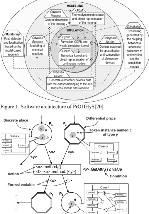
This environment provides a library of classes dedicated to the dynamic hybrid simulation of processes. The primal contribution of these works consisted in determining and designing the
foundation buildings classes. Currently, this library is made up of more than one thousand classes distributed into three functional layers and nine modules (Figure 1):
- The internal layer corresponds to the simulation kernel of the platform. It provides the basic elements allowing the simulation of any dynamic systems. Today, this layer includes:
o the module Disco[18],[52], which constitutes the numerical kernel of the systems and allows an object representation of the continuous mathematical models; it provides a set of solvers and integrators (DAE, NLAE);
o the module Hybrid[19] which contains the set of classes used for the description of the ODPN formalism as well as the hybrid simulation kernel.
- The second layer includes a set of classes allowing the modelling of processes. The "modelling" layer rests on the "simulation" layer and provides a set of general and autonomous entities which can be exploited by any user who wishes to build its own simulation system or prototype. This layer includes:
o the module ATOM[17] which constitutes the thermodynamic data base of the system; it is based on an object representation of the material and allows the computing of thermodynamic properties.
o the module Odysseo[53] which gathers the elementary and generic entities allowing the modelling of a process. It is divided into three sub-modules:
the sub-module Process which gathers a set of often abstract classes, corresponding to a very general description of the process;
the sub-module Reaction which allows the modelling of chemical reactions;
the sub-module Device which gathers the "concrete" elementary devices.
o the module CompositeDevice which gathers devices resulting from the composition and the specialisation of the elementary devices defined in the module Odysseo.
- The higher layer corresponds to a set of classes dedicated to the process supervision. This “supervision” layer rests on the "simulation" and “modelling” layers and provides a set of entities allowing the realization of monitoring studies. Then, this layer includes:
o the module Scheduling[54], which couples the simulation module with stochastic optimization methods;
o the module PrODHySAEM[20] (Process Object Dynamic Hybrid Simulator for
Abnormal Event Management), which contains a set of classes, in charge of
the management of the monitoring studies of the processes.
The interest to separate the "simulation" and the "modelling" layers is to build platforms dedicated to various field of applications (mechanical, electronic, etc.) only by developing the suitable engineering "modelling" layer.
2.2 ODPN formalism
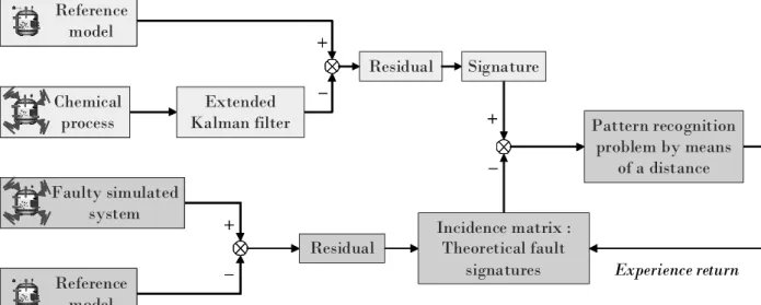
A detailed description of this formalism can be found in [19][20]. The PrODHyS components allow a modular and hierarchical modelling of different processes. In consequence, the object concepts and the Petri nets have been exploited in a combined approach in the ODPN formalism. It consists in making interact these features according to two manners (Figure2). Firstly it aims at “introducing the objects into Petri nets”. The subjacent philosophy is to model a subsystem by a single Petri net, which handles individualised tokens carrying information. The second approach is based on “the introduction of Petri nets into objects” to describe the internal behaviour of the object (cf. class t). The marking of the Petri net indicates the current state of the object.
The ODPN formalism makes collaborate, within the same structure, DAE systems to describe the continuous evolution of the system with a high level Petri net used to specify the legal sequences of commutation between this set of DAE systems. Moreover, the integration of the DAE system of a differential place can require several tokens of the same type and/or of different types. In this case, the consistency must be assured by the modelling or validated by the simulation. Thus, the Petri net can be seen as DAE monitor. It allows the dynamic creation of a unique simulation model, whose size and structure change between two events (no fixed size of state vector). Besides the resolution of the DAE system (integration based on the Gear method) and of the discrete models (Petri net player specific to this class), the kernel manages other functionalities, such as the exact calculation of the commutation times, the state failing, the checking of the consistency of the new models generated after the commutation, the initialisation of the state variables and their derivatives[19]…
2.3 Process modelling with PrODHyS
To carry out the simulation of such a system, it is necessary to model the command part (the supervisor) and the operative part (the process) at the same time. The model is a priori specific to the recipe and the considered process topology. So, it is completely dissociated from the model of devices, since this model must be reusable whatever the studied context (concept of component).
Moreover, the material model is dissociated from the device which contains the material. These different models are merged just at the time of the instantiation of the simulation model, according to the present state of the process. As a result, a hierarchical organization of models is introduced: the command level contains the recipe to execute, whereas the process level simulates the process behaviour[19][20]. At this level, two kinds of entity are
distinguished:
- The active entities: they are devices, whose Petri net has one or several command places, such as the valves, the pumps, the energy feeds, etc.
- The passive entities: they are entities, whose Petri net doesn’t have command place (so without direct connection with the recipe Petri net) such as storage tanks, reactors or material.
The evolution of the different models is conditioned by two distinct kinds of event. On the one hand, we have “extern” events, which entail the controlled commutations. These are the signals exchanged between the command level and the process level. So they correspond either with commands send from the recipe Petri net in order to manage the active entities, or with the occurrence of a state event (detection of a threshold) or a temporal event. These events are defined by the user and clearly appear in the recipe Petri net. In this way, all the Petri nets of the command level manage all the Petri nets of the process level and can be compared to the GRAFCET in a DCS of the command level. On the other hand, we have the “intrinsic” events, whose occurrence depends only on the spontaneous process evolution. For example, these autonomous commutations correspond with the state change of a passive entity or with the change from the liquid to the vapour state when the boiling temperature is reached. These commutations don’t appear on the recipe Petri net (so the user doesn’t specify them) and are dealt with exclusively in the model of the concerned entity (device or material).
3 Supervision module
In chemical plants faults may cause process performance degradation (for example lower product quality) or fatal accidents (for instance the runaway scenario). Fault monitoring could prevent from these undesirable consequences. Several fault diagnosis approaches have been mainly proposed for steady-state processes operating. Nevertheless, application of these techniques to batch processes remains a challenging task, because of their hybrid and
nonlinear dynamics[55]. Among model-based approaches, observer-based schemes have been
used in numerous application fields.
3.1 Architecture
For this purpose, the simulation model of PrODHyS is used as a reference model to implement the functions of detection and diagnosis. The simplified principle of this system is shown on the Figure 3. A description of this methodology can be found in [20],[56].
In order to obtain an observer of the physical system, a real-time simulation is done in parallel. So, a complete state of the system will be available at any time. Thus, it is based on the comparison between the predicted behaviour obtained thanks to the simulation of the reference model (values of state variables) and the real observed behaviour (measurements from the process correlated thanks to the Extended Kalman Filter). Detection is realized by comparison with fixed thresholds. For a consistent execution of this task, the measurements must be filtered in order to eliminate the noise. The filter used here is the Extended Kalman Filter.
3.2 Implementation of the Extended Kalman Filter
In a model-based approach, one of the first problems is to differentiate the deviations due to a failure, from those related to the inherent disturbances of the process. For the inherent disturbances, we distinguish the measurement noises, the variations of the operating conditions and the parametric uncertainties. Thus, the failures, which we want to detect, are: the structural variations, which are generated by the wear of the devices, the failures of the actuators, and the failures of the sensors.
In order to mask the inherent disturbances and to avoid the false alarms, we have used an extended Kalman filter. A description of this filter can be found in [20]. Figure 4 illustrates the steps of the estimation of the system state. There are two main steps:
- the prediction, which corresponds to the “a priori” estimation
- and the correction, which corresponds to the “a posteriori” estimation.
Thus, the state vector is initially evaluated from the estimate of the previous step. Then, it is corrected by the measurements in the correction step. Both steps compose of an iterative of this filter (Figure 5).
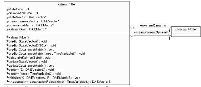
This filter is described by the class kalmanFilter (Figure 5). Its initialization is carried out by the call of the method initialize. The class kalmanFilter has two attributes _systemDynamic and _measurementDynamic of type dynamicModel. The first attribute represents the dynamic of the system and the second represents the dynamic of the observations. Then, the dynamic models are not explicitly included in the computation of the filter, since they are defined by the class dynamicModel. Thus, the procedure applies to any type of system: the linear physical system or not and the linear dynamics of the observations or not.
The execution of the filter is made through the call of the method perform (Figure 6). This method gathers the two steps of the Kalman filter:
- The methods predictStateVector and predictCovarianceMatrix manage the prediction step,
- and for the correction step, these are the methods calculateKalmanGain,
updateStateVector and updateCovarianceMatrix. 3.3 Simulation in parallel
According to the suggested architecture (Figure 3), our approach requires the on-line simulation in parallel of a reference process and of the extended Kalman filter. A main recipe is generated and groups together these both recipes. In order to distinguish the places and the transitions of these Petri nets, a prefix is added to their names:
- “M-“ for the recipe of the reference model, - “K-“ for the recipe used by the Kalman filter.
Figure 7 represents the general concept. When the transition TRBEGIN is fired, each place
BEGIN of the Petri nets is marked. When the horizon time of the simulation is passed, the
place END is marked.
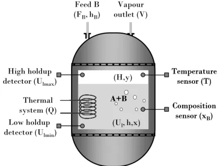
4 Application
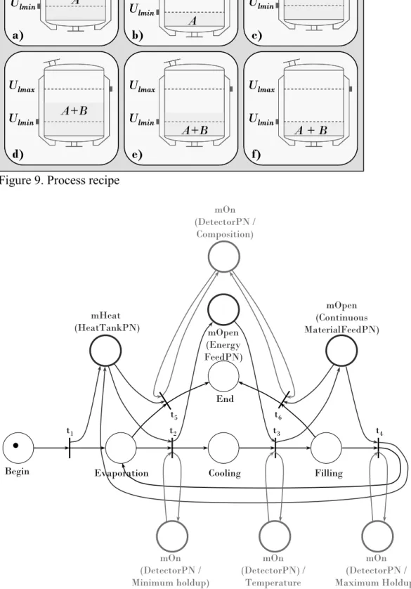
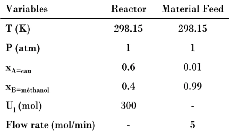
A didactic example, shown on Figure 8, has been chosen in order to illustrate the proposed approach. This is the process of addition-evaporation. This is generally used to change solvents. The operation conditions are listed in the Table 1. The values of the minimum and maximum hold-ups are respectively 200 and 800 moles. Before each addition of solvent, the reactor is cooled up to the temperature of 300.15K. The pressure is supposed to be constant during this operation. The goal of this process is to have a molar composition of methanol in the reactor at 0.95.
4.1 Process recipe description
The operating of the substitution of the solvent A for the solvent B follows the following recipe:
1. The initial holdup is higher than the minimum holdup (Ulmin). The first step consists of the concentration of the solvent A. Figure 9 a) represents this step. The mixture is heated until its boiling point of and its vaporization is partial. This stage takes place, until the minimum holdup (Ulmin) is reached.
2. The reactor is then filled by a continuous feed (Figure 9 b)). A quantity of the substitution solvent (solvent B) is thus added to the mixture.
3. Then, two evolutions are possible (Figure 9 c)):
o If the wanted quality of the product B is reached, the operating sequence is finished.
o Otherwise, the feed is closed when the maximum holdup is reached (Ulmax). The operating sequence continues with a new evaporation step (step4).
4. The mixture is then evaporated (Figure 9 d)). The mixture is heated until its boiling point of and its vaporization is partial.
5. Next, two evolutions are possible (Figure 9 e)):
o If the wanted quality of the product B is reached, the operating sequence is finished.
o Otherwise, the evaporation in the reactor continues until the minimum holdup is reached. Then, the cooling of the mixture takes place.
6. The cooling is maintained until the specified temperature is reached. Figure 9 f) represents this step. The next operating sequence is a new addition stage (step 2). Its recipe describes a succession of evaporations and additions of the new solvent, until the wanted final quality of the substitution solvent is reached.
4.2 Mathematical model
The mathematical model of this system at the thermodynamic equilibrium and in its maximal state (i.e., liquid/vapour) is as follows.
0 V F dt dU B l (1) 0 ) . ( i i B B i l F x Vy dt x U d c n i 1, (2) 0 ) ( F h VH Q dth U d B B l (3) 0 c ml l l USV h (4)
0 . i i i K x y i ,1nc (5) c n i 1(xi yi) 0 (6) 0 ) y , x , , ( PT mK Ki i i ,1nc (7) 0 ) x , , ( PT mh h (8) 0 ) y , , ( PT mH H (9) 0 ) , , (T P x mV Vml ml (10) 0 ) , , (T P y mV Vmv mv (11)
The outlet vapour being open on the outside, the pressure P is supposed to be constant and the vapour holdup Uv is neglected in front of Ul. Equations (1), (2) and (3) represent the material and energy balances respectively. Equation (4) determines the liquid height hl according to the
tank area Sc, the molar volume of the liquid phase Vml and the liquid holdup Ul. Equations (5) and (6) represent the liquid/vapour equilibrium. Finally, equations (7), (8), (9), (10) and (11) are the models used for the liquid/vapour equilibrium constants Ki, the liquid enthalpy h, the vapour enthalpy H, the liquid molar volume Vml and the vapour molar volume Vmv within the tank.
4.3 Recipe Petri net
The recipe of this process is described by the Petri net of the Figure 10. Initially, the tank contains the two solvents and the liquid holdup is contained between the minimum and maximum values. The material and energy feeds are closed and the detectors are in position off.
- The marking of the place Begin allows the beginning of the operation. Then, the transition
t1 is fired. The marking of the place mHeat conveys the order sent by the recipe to the energy system, and the marking of the place Evaporation means that the first step takes place. Next, two evolutions are possible:
o The composition of the new solvent reaches the target value. This information is transmitted to the recipe by the marking of the place mOn of the composition detector. In this case, the transition t5 is fired and allows the marking of the place End.
o The minimum holdup is reached. This information is transmitted to the recipe by the marking of the place mOn of the low holdup detector. Then, the transition t2 is fired and allows the marking of the place Cooling.
- The cooling is maintained until a preliminary specified temperature is reached. This event is transmitted to the recipe by the temperature sensor (transition t3).
- The next step consists in the adding of the new solvent. This is represented by the marking of the place Filling. Then, two evolutions are possible:
o The composition of the new solvent reaches the target value. This event is detected by the composition detector (transition t6).
o The maximum holdup is reached. This information is transmitted to the recipe by the marking of the place mOn of the high holdup detector. The operation continues with a new evaporation step (transition t4).
5 Adjustments of the filter
To perform a monitoring of a process, some off-line adjustments must be made. As a matter of fact, the values of the covariance matrices of the model and measurement disturbances have to be determined.
The system observations are obtained by the use of specific sensors. So, the measurement mistakes are relatively well-known by the manufacturer or by experimentation. Thus, it is easy to define an estimate of the measurement covariance matrix.
5.2 Model disturbances
Before activating the extended Kalman filter, it is important to estimate the sensitivity of the filter to the model parameters. Thus, these works are based on a sampling scheme for the measurement perturbations and the model noise. This allows the estimation of the statistics of the model uncertainties. Then, we made numerous simulations during which uncertainties are generated. These uncertainties are obtained by disturbing at random one of the input parameters or one of the modelled physical processes. Therefore, a sampling of possible trajectories of the model is established. This method is based on the following hypothesis: the sampling average corresponds to the best estimate of the system state (our model is supposed to be unbiased), and the dispersion around this average corresponds to a measurement of the mistake of this estimate[57],[58]. Thus, we estimate a wide uncertainty on the modelled physical processes, in order to be certain that the obtained dispersion includes the real behaviour of the system. Then, if the behaviour of the system goes beyond this distribution, its behaviour is abnormal. So, the detection thresholds are determined according to the model disturbances. In practice, we made a set of simulations in parallel by adding a noise to the process or to a parameter, uniformly distributed between -σ and σ (where σ is the typical range). Thus, it is possible to deduce the characteristics (average and typical range) of the dispersion of the system distribution function. Table 2 summarizes the applied uncertainties.
For example, Figure 11 represents the results obtained by modifying the initial value of the reactor liquid holdup. The curves represent the time evolution of the balanced typical ranges of the following state variables: the reactor liquid holdup (Ul), the molar liquid composition of the product B (xB) and the temperature (T). Notice that these typical ranges are normalized in order to compare them between themselves. The system states are also illustrated on Figure 11. Notice that the evolution changes of the typical ranges are linked to the change of the system state. For example, at t= 258 min, we note a first peak of the typical range of the temperature. This corresponds to the change from the state Evaporation to the state Filling. Besides, the two following peaks (for the liquid holdup and the molar liquid composition of the product B) point out the change from the state Filling to the state Cooling and at t = 390 min, the third peak underlines the stopping of the system cooling.
Consequently, the model is more sensitive to the input parameter uncertainties during the transient modes. Thus, during these modes, the use of the extended Kalman filter is importance.
This study is reproduced for all the uncertainties exposed in Table 2. Then, a value of the modelling uncertainties is estimated (Table3).
5.3 Initialization of the extended Kalman filter
We point out that our works are based on dynamic simulation. Thus, during a simulation, there are several models of the system. So, for each model change, it is necessary to initialize judiciously the state vector and the covariance matrix.
5.3.1 Initialization of the state vector
Since our variables are continuous, the state vector of the new model is initialized with the value of the previous state (Figure 12).
5.3.2 Initialization of the covariance matrix
The covariance matrix of the modelling uncertainties of the new model could be initialized with the value of the previous model. This would mean that we have as much confidence in the new model as in the old one. However, the model disturbances are one of the most important causes in the divergence of the Kalman filter. This divergence is due to the fact that the filter has a too much confidence in the model. This is the case when the model noise is low. As a matter of fact, the terms of the covariance matrix representing the model disturbances and those of the gain matrix decrease. Thus the filter doesn’t take into account the observations. Thus, it is necessary to adjust intelligently the covariance matrices, in order to solve this problem. One of the mainly used solutions is to increase the uncertainty of the model. For this, we suggest that, for each model change, the covariance matrix of the new model is initialized by the initial value of the covariance matrix of (Figure 12), i.e. the value of Table 3.
6 Results
The simulations of the reference model are first presented. Then, the results of the detection are exposed.
6.1 Simulation of the reference model
The simulation of the reference process is made. The dynamics are illustrated on Figure 13: they represent respectively the time evolutions of the liquid compositions.
The final molar methanol composition in the tank is equal to 0.95 (Figure 13) and was obtained during the adding of the new solvent. The total operation requires four additions and four evaporations.
6.2 State reconciliation
Figure 14 shows .that the estimated state fits the reality. Moreover, in the model changes, the initialization of the extended Kalman filter allows its convergence. Thus, the state is well estimated during the transient modes.
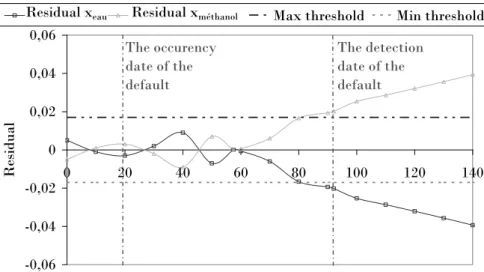
6.3 Detection
This process is a system based on thermal phenomena. A fault on the tank thermal system is a risk for the success of this operation. That is why, it is important to detect it as soon as possible.
We remind that the thresholds for the detection correspond to the model uncertainties obtained by the adjustment of the Extended Kalman filter (Table 3). A fault on the heating energy feed of the reactor takes place at t = 20 min. This energy feed provides a heat quantity lower than the nominal one. Figure 15 shows the detection step. It illustrates the residuals evolution linked to the liquid composition of water and methanol. From t = 80 min, the both residuals go beyond the area of the nominal performance. The diagnosis is launched at t = 95 min.
7 Conclusion
In this paper, the feasibility of using the Extended Kalman Filter as a tool for fault detection is described. The method developed in this study rests on a hybrid dynamic simulator PrODHyS. This simulator is based on an object oriented approach. It brings many advantages in terms of software quality (extensibility, reutilisability, flexibility), but especially in terms of modelling thanks to a hierarchical and modular description which is both abstracted and close to reality. Then, PrODHyS provides software components intended to model and simulate more specifically the industrial processes. The implementation of a formalism on high level of abstraction associated with powerful numerical methods of integration led to the construction of a robust hybrid dynamic simulator. In this communication, the potentialities of PrODHyS are illustrated through the modelling and the simulation of a process. The works in progress aim at integrating this simulation model within a model based diagnosis system. Different diagnosis approaches mixing model-based and data classification techniques will be studied and compared.
Appendix A. Nomenclature
Fi Liquid flow rate (mol/min)
hi Liquid enthalpy (J/mol)
Hi Vapour enthalpy (J/mol)
Ki Equilibrium constant nc Constituent number P Pressure (Pa) Qi Energy quantity (W) Sc Area (m²) T Temperature (K)
Ul Liquid holdup (mol)
Uv Vapour holdup (mol)
Vi Vapour flow rate (mol/min)
Vml Liquid molar volume (m3/mol)
Vmv Vapour molar volume (m3/mol)
xi Liquid composition
References
[1] J. Zaytoon, Systèmes dynamiques hybrides, Hermès Sciences publications, 2001 ; p 378
[2] M.S. Branicky, Studies in hybrid systems: Modeling, Analysis and Control. PhD-thesis, MIT, Massachusetts, USA, 1995
[3] J. Buisson, H. Cormerais, Journal Européen des systèmes automatisés, 1998, 32 (9-10), 1047-1072
[4] J. Le Bail, H. Alla, R. David Proceedings of the European Control Conference, France,
1991 ; pp. 1472-1477
[5] I. Demongodin, Discrete Event Dynamic Systems: Theory and Applications, 2001, 11 (1-2), 137-162
[6] B. Berthomieu; M. Menasche, IFIP Congress Series, 1983, 9, 41-46 [7] R. Alur, D.L. Dill, Theoretical Computer Science, 1994, 126 (2), 183-225
[8] R. Alur, C. Courcoubetis, N. Halbwachs, T.A. Henzinger, P.H. Ho, X. Nicollin, A. Olivero, J. Sifakis, S. Yovine, Theoretical Computer Science, 1995, 138, 3-34
[9] Y. Kesten, A. Pnueli, Lecture Notes in Computer Science (LNCS), 1992, 571
[10] C. Valentin-Roubinet, Proceedings of Automation of Mixed Processes (ADPM 98), March 19-20, Reims, France, 1998, pp. 142-149
[11] R. Champagnat, H. Pingaud, H. Alla, C. Valentin-Roubinet, J.M. Flaus, R. Valette, European Journal of Automation, 1998, 32 (9-10), 1233-1253
[12] P.I. Barton, C.C. Pantelides, AIChE Journal, 1994, 40, 966-979
[13] M. Andersson, Object-Oriented Modelling and Simulation of Hybrid Systems, PhD-Thesis, Lund Institute of Technology, Lund, Sweden, 1994
[14] K. Wöllhaf, M. Fritz, C. Schulz, S. Engell, Supplement to Computers and Chemical Engineering, 1996, 20(972), 1281-1286
[15] A. Deshpande, A. Göllü, L. Semenzato, IEEE Transaction Automatic Control special issue on Hybrid Systems, 1998
[16] G. Fábián, D.A. Van Beek, J.E. Rooda, Integration of the Discrete and the Continuous
Behaviour in the Hybrid Chi Simulator, European Simulation Multiconference, Manchester,
UK, 1998
[17] L. Jourda, X. Joulia, B. Koehret, Computers and Chemical Engineering, 1996, Suppl. A (20), S157-S164
[18] A. Sargousse, Noyau numérique Orienté-Objet dédié à la Simulation des systèmes
Dynamiques Hybrides, PhD-Thesis, INP, Toulouse, France, 1999 ; p 207
[19] J. Perret, G. Hétreux, J.M. Le Lann, Control Engineering Practice, 2004, 12 (10), 1211-1223
[20] N. Olivier-Maget, G. Hétreux, J.M. Le Lann, M.V. Le Lann, Chem. Eng. Process,
2008, doi:10.1016/j.cep.2007.12.009
[21] A. Birouche, Contribution pour la synthèse d’observateurs pour les systèmes
dynamiques hybrides, PhD-Thesis, Institut National Polytechnique de Lorraine, Nancy,
France, 2006 ; p 153
[22] Y. Chetouani, Asia Pacific Journal of Chemical Engineering, 2008, 3, 597-605
[23] R.N. Clark, D.C. Fosth, IEEE Transactions on Aerospace and Electronic Systems
1975, AES-11, 465-473
[24] R.N. Clark, Proceedings of the 18th IEEE-CDC, Fort Lauderdale, Florida, USA, 1979 ;
pp. 237-241
[25] R.N. Clark, State estimation schemes for instrument fault detection. Fault Diagnosis in
Dynamic Systems: Theory and application, ed. R. Patton, P. Frank and R. Clark, Prentice
[26] P.M. Frank, Fault diagnosis in dynamic systems via state estimation – a survey, S. Tzafestas, M. Singh, G. Schmidt (Eds.), Systems fault diagnostics, reliability and related knowledge-based approaches, 1987, 1, 35-98
[27] R.J. Patton, J. Chen, Proceedings of IFAC conference on Fault Detection, Supervision and Safety for Technical Processes, Baden-Baden, Germany, 1991 ; pp. 65-81
[28] J.F. Magni, P. Mouyon, Proceedings of the 30th IEEE-CDC, December 11-13, Brighton, UK, 1991, 3, 2236-2241
[29] A.J. Krener, System Control Letter, 1984, 5, 181-185
[30] R. Marino, P. Tomei, Nonlinear control design., London, New York, Prentice Hall, Information and system sciences, 1995
[31] G. Bastin, M. Gevers, IEEE Trans. on Automatic Control, 1998, 33(7), 650-658 [32] C. De Persis, A. Isidori, IEEE Trans. on Automatic Control, 2001, 46 (6), 853-865 [33] D. Maquin, V. Cocquempot, J.P. Cassar, M. Staroswiecki, J. Ragot, Proceedings of IEEE Int. Symposium on Diagnostics for Electrical Machines, Power Electronics and Drives, SDEMPED’97, Carry-le-Rouet, France, 1997 ; pp. 270-276
[34] A. Xu, Observateurs adaptatifs non-linéaires et diagnostic de pannes, PhD-Thesis, Université de Rennes 1, Rennes, France, 2002 ; p 131
[35] D. Hengy, P.M. Frank, Proceedings of the IFAC Workshop on Fault Detection and Safety in Chemical Plants, Kyoto, Japan, 1986 ; pp. 153-157
[36] P.M. Frank, Fault diagnosis in dynamic systems via state estimation – a survey, S. Tzafestas, M. Singh, G. Schmidt (Eds.), Systems fault diagnostics, reliability and related knowledge-based approaches, 1987, 1, 35-98
[37] K. Adjallah, Contribution au diagnostic de systèmes par observateur d’état, PhD-Thesis, Institut National Polytechnique de Lorraine, Nancy, France, 1993 ; p 153
[38] A.H. Jazwinski, Stochastic Processes and Filtering Theory, Libri, 1970 ; p376 [39] K. Reif, R. Unbehauen, IEEE Trans. on Signal Processing, 1999, 47 (8), 2324-2328 [40] G.A. Einicke, L.B. White, IEEE Trans. on Signal Processing, 1999, 47 (9), 2596-2599 [41] J.P. Gauthier, H. Hammouri, S. Othman, IEEE Trans. on Automatic Control, 1992, 37, 875-880
[42] R. Nikoukhah, IEEE Trans. on Automatic Control, 1998, 43(2), 229-231 [43] K. Salahshoor, M. Mosallaei, M. Bayat, Measurement, 2008, 41, 1059-1076
[44] G.A. Einicke, L.B. White, IEEE Trans. on Signal Processing, 1999, 47 (9), 2596-2599 [45] K. Reif, R. Unbehauen, IEEE Trans. on Signal Processing, 1999, 47 (8), 2324-2328 [46] V. Venkatasubramanian, R. Rengaswamy, K. Yin, S.N. Kavuri, Computers and Chemical Engineering, 2003, 27, 293-346
[47] M. Basseville, Proceedings of IFAC Safeprocess 2003. Washington, DC, 2003. [48] R.K. Mehra, J. Peschon, Automatica, 1971, 5, 637-640
[49] S. Simani, C. Fantuzzi, Mechatronics, 2006, 16, 341-363
[50] G. Welch, G. Bishop, An introduction to the Kalman filter, Technical Report TR 95-041, University of North Carolina, 1995
[51] R. Xiong, P.J. Wissman, M.A. Gallivan, Computers and Chemical Engineering, 2006, 30, 1657-1669
[52] J.M. Le Lann, Des mathématiques à la simulation dynamique robuste des procédés :
le traitement algébro-différentiel des équations EDA, Habilitation à Diriger les Recherches,
INP, Toulouse, France, 1999
[53] A. Moyse, Odysseo : plate-forme orientée-objet pour la simulation dynamique des
procédés, PhD-Thesis, INP de Toulouse, France, 2000 ; p 260
[54] G. Hétreux, F. Fabre, R. Thery, J.M. Le Lann, Récents Progrès en Génie des Procédés, ISBN 2-910239-70-5, Ed. SFGP, Paris, France, 2007, 96
[55] F. Pierri, G. Paviglianiti, F. Caccavale, M. Mattei. Engineering Applications of Artificial Intelligence, 2008, 21, 1204-1216
[56] N. Olivier-Maget, Surveillance des Systèmes Dynamiques Hybrides : Application aux
procédés, PhD-Thesis of the Toulouse University (INSA), France, 2007 ; p 344
[57] G. Evensen, Ocean Dynamics, 2003, 53, 343-36
[58] V. Maget, Développement et comparaison de méthodes d’assimilation de données
appliqués à la restitution de la dynamique des ceintures de radiation de la Terre. PhD-Thesis
of the Toulouse University (École Nationale Supérieure de l’Aéronautique et de l’Espace), France, 2007 ; p 223
SUPERVISION
Hybrid
DISCo
Numerical kernel and object representation of continuous models SIMULATION MODELLING ATOM Odysseo Process
Formalism ODPN and Hybrid simulation kernel
Scheduling Fault detection and localisation based on the model-based approach Monitoring General description of the process Thermodynamic database and object representation
of the material Odysseo Reaction Modelling of chemical reactions Composite Device Devices obtained by specialisation and composition of elementary devices Odysseo Device
Concrete elementary devices built with the classes belonging to the
sub-modules Process and Reaction
Scheduling generated by the coupling between a stochastic procedure of optimization and the simulation module SUPERVISION Hybrid DISCo
Numerical kernel and object representation of continuous models SIMULATION MODELLING ATOM Odysseo Process
Formalism ODPN and Hybrid simulation kernel
Scheduling Fault detection and localisation based on the model-based approach Monitoring General description of the process Thermodynamic database and object representation
of the material Odysseo Reaction Modelling of chemical reactions Composite Device Devices obtained by specialisation and composition of elementary devices Odysseo Device
Concrete elementary devices built with the classes belonging to the
sub-modules Process and Reaction
Scheduling generated by the coupling between a stochastic procedure of optimization and the simulation module
Figure 1. Software architecture of PrODHyS[20]
y x <x> <y> <t> <x> Objet1 methode1 methode2 methode4 methode3 Class y methode1 method1 methode2
method2 methodemethod44
methode3 method3 <x>.method2() <t>=<x>.method1(<y>) Objet2 methode1 methode2 methode4 methode3 Class x methode1 method1 methode2
method2 methodemethod44
methode3 method3 <x>.GetAttr1() value t <y> y Class t method1 method2 method3 method4 method7 method6 method5
Discrete place Differential place
P1 P2 P3 P4 a b c d
Token instance named c of type y Condition Action Typed token Formal variable yyy x <x> <y> <t> <x> Objet1 methode1 methode2 methode4 methode3 Class y methode1 method1 methode2
method2 methodemethod44
methode3 method3 Objet1 methode1 methode1 methode2
methode2 methodemethode44
methode3 methode3 Class y methode1 method1 methode2
method2 methodemethod44
methode3 method3 <x>.method2() <t>=<x>.method1(<y>) Objet2 methode1 methode1 methode2
methode2 methodemethode44
methode3 methode3 Class x methode1 method1 methode2
method2 methodemethod44
methode3 method3 <x>.GetAttr1() value t <y> yy Class t method1 method2 method3 method4 method7 method6 method5 Class t method1 method1 method2 method2 method3 method3 method4 method4 method7 method7 method6 method6 method5 method5
Discrete place Differential place
P1 P2 P3 P4 a b c d
Token instance named c of type y
Condition Action
Typed token Formal variable
Residual Residual Pattern recognition problem by means of a distance Incidence matrix : Theoretical fault signatures Signature Extended Kalman filter – + – + Experience return Faulty simulated system A+B A+B Faulty simulated system A+B A+B A+B A+B Chemical process A+B A+B Chemical process A+B A+B A+B A+B Reference model A+B A+B Reference model A+B A+B – + – + – + – + Reference model A+B A+B Reference model A+B A+B
Figure 3. Supervision Architecture
Pr ed ictio n Tim e up date C or rec tio n Me as ur em en t u pd ate
Initialization with the previous filtered estimate state
Available measurement ? No Yes
Computation of the Kalman gain Update of the state estimate Update of the error covariance Computation of the Kalman gain
Update of the state estimate Update of the error covariance
Projection of the state ahead Projection of the error covariance
ahead
Figure 5. Class diagram of the extended Kalman filter
Perform method
Correction step Prediction step
Measurement Vector
1. Call of the method predictStateVector 2. Call of the method predictCovarianceMatrix
If there is a measurement of the system
3. Call of the method calculateKalmanGain 4. Call of the method updateStateVector 5. Call of the method updateCovarianceMatrix
Estimated state vector
END BEGIN
TRBEGIN
TREND2 t ≥ th
With thsimulation horizon time RECIPE OF THE REFERENCE PROCESS
M-BEGIN REFERENCE FLOWSHEET FEED C1 C2 P1 V2 V1 hST1 hST1 QP1 QP1 hST2 hST2 QV2 QV2 QV1 QV1 DP1 DP1 OV1 OV1 OV2 OV2 p1 p2 DECT2 DECT1 ∑1 D∑1 D∑1
RECIPE OF THE KALMAN FILTER K-BEGIN REFERENCE FLOWSHEET FEED C1 C2 P1 V2 V1 hST1 hST1 QP1 QP1 hST2 hST2 QV2 QV2 QV1 QV1 DP1 DP1 OV1 OV1 OV2 OV2 p1 p2 DECT2 DECT1 ∑1 D∑1 D∑1 t ≥ th TREND1
Figure 7. Petri net of the main recipe
Feed B (FB, hB) outlet (V)Vapour Thermal system (Q) Composition sensor (xB) Composition sensor (xB) Low holdup detector (Ulmin) High holdup
detector (Ulmax) TemperatureTemperaturesensor (T)sensor (T)
(Ul, h,x)
(H,y)
A+B
Ulmin A Ulmax Ulmin A Ulmax FB Ulmin A+B Ulmax Ulmin A+B Ulmax Ulmin A+B Ulmax Ulmin A + B Ulmax a) b) c) d) e) f) Ulmin A Ulmax Ulmin A Ulmax Ulmin A Ulmax FB Ulmin A Ulmax FB Ulmin A+B Ulmax Ulmin A+B Ulmax Ulmin A+B Ulmax Ulmin A+B Ulmax Ulmin A+B Ulmax Ulmin A+B Ulmax Ulmin A + B Ulmax Ulmin A + B Ulmax a) b) c) d) e) f)
Figure 9. Process recipe
mOn (DetectorPN / Minimum holdup) mHeat (HeatTankPN) Filling Cooling Evaporation Begin mOpen (Energy FeedPN) mOpen (Continuous MaterialFeedPN) mOn (DetectorPN) / Temperature mOn (DetectorPN / Maximum Holdup) mOn (DetectorPN / Composition) End t2 t3 t4 t1 t5 t6
0 0,02 0,04 0,06 0,08 0,1 0,12 0 500 1000 1500 2000 2500 3000 3500 4000 4500 5000 Time (min) Normed typical range Variables: Ul xB T
System states: Evaporation Filling Cooling
Ul xB
Figure 11. Results of the sampling method
Initialization Kalman filter algorithm INITIAL MODEL X0 P0 Initialization • X : previous state • P : initial state Kalman filter algorithm MODEL CHANGE P0
…
0 0,1 0,2 0,3 0,4 0,5 0,6 0,7 0,8 0,9 1 0 1000 2000 3000 4000 5000 Time (min) Mola r com positio ns -2000 -1500 -1000 -500 0 500 1000 1500 Hea ting and co oli ng ( W) Flo w rate o f the ma ter iel feed (mo l/mi n) xeau xméthanol Heating Cooling Flow rate * 200 xA xB
Figure 13. Results of the reference process
0 0,1 0,2 0,3 0,4 0,5 0,6 0,7 0,8 0 500 1000 1500 2000 Time (min) Comp ositio n Xeau Xeau FK
State evaporation State cooling
State filling
xeau xeau,FK
-0,06 -0,04 -0,02 0 0,02 0,04 0,06 0 20 40 60 80 100 120 140 Time (min) Residual
résidu xeau résidu xméthanol Max threshold Min threshold
The occurency date of the default The detection date of the default
Residual xeau Residual xméthanol
1 1 P (atm) 0.01 0.6 xA=eau -300 0.4 298.15
Reactor Material Feed Variables
5 Flow rate (mol/min)
-Ul(mol) 0.99 xB=méthanol 298.15 T (K) 1 1 P (atm) 0.01 0.6 xA=eau -300 0.4 298.15
Reactor Material Feed Variables
5 Flow rate (mol/min)
-Ul(mol) 0.99 xB=méthanol 298.15 T (K)
Table 1. Operating conditions
Cooling energy quantity
Uncertainties
Composition threshold Maximum holdup threshold Minimum holdup threshold Composition in the reactor
Heating energy quantity Flow rate of the material feed Liquid retention in the reactor Parameters
Cooling energy quantity
Uncertainties
Composition threshold Maximum holdup threshold Minimum holdup threshold Composition in the reactor
Heating energy quantity Flow rate of the material feed Liquid retention in the reactor Parameters 20 , 0 N avec Ulref 5 . 0 , 0 N avec FBref 05 . 0 , 0 N avec xrefA 05 . 0 , 0 N avec xrefB 20 , 0 N avec Ulrefmax 20 , 0 N avec Ureflmin 100 , 0 N avec Qcoolref 100 , 0 N avec Qrefheat
Table 2. Uncertainties of the parameters and of the initial conditions
30 mol 0.015 0.015 0.015 0.01 3.5 K yB xA yA xB T Ul 30 mol 0.015 0.015 0.015 0.01 3.5 K yB xA yA xB T Ul Table 3. Modelling uncertainties