Statistical analysis of fish ladder attractivity on the Nord-Est Sainte-Marguerite River.

S

N

-E

S

-M

R

by

Danielle Frechette

André St-Hilaire

Normand Bergeron

SCIENTIFIC REPORT #R1834

Institut national de la recherche scientifique (INRS)

Centre Eau, Terre et Environnement

i

Reference to be cited :

Frechette, D., A. St-Hilaire, N.E. Bergeron. 2019. Statistical analysis of fish ladder attractivity on the Nord-Est Sainte-Marguerite River. INRS Scientific Report R1834. iv+17 pages.

© INRS, Centre - Eau Terre Environnement, 2019 Tous droits réservés

ISBN : 978-2-89146-915-9 (version électronique)

Dépôt légal - Bibliothèque et Archives nationales du Québec, 2019 Dépôt légal - Bibliothèque et Archives Canada, 2019

ii

T

C

List of Figures ...iii

List of Tables ... iv

1. Introduction ... 1

2. Methodology ... 2

2.1 Fish count data ... 2

2.2 Environmental Data ... 2

2.3 Modeling Presence-Absence Data ... 6

2.4 Modeling Daily Count Data ... 8

3. Results ... 9

3.1 Modeling Presence-Absence Data ... 9

3.2 Modeling Count Data ... 12

4. Conclusions ... 14

5. Acknowledgements ... 16

iii

L

F

Figure 1. Temperature measured at the station Joe Savard (black line) and at the fish ladder (gray line) during summer 2015 (left) and 2016 (right). ... 3 Figure 2. Linear relationship between river temperature measured at JoeSavard and at the fish ladder during summer 2015 and 2016, given by the equation y = 0.9844x - 0.0065 (R2 = 0.9933, p < 2.2e-16). ... 4 Figure 3. Residual plots used to evaluate assumptions for the regression between river temperature measured at JoeSavard and measured at the fish ladder during the summers of 2015 and 2016. 4 Figure 4. River temperature measured at Joe Savard (red line) and river temperature estimated for the fish ladder from the equation y = 0.9844x - 0.0065 (R2 _{= 0.9933, p < 2.2e-16). ... 5}

Figure 5. River temperature at the fish ladder estimated from measured temperature at JoeSavard (first and second rows) and directly measured at the fish ladder (bottom row). ... 5 Figure 6. Distribution of “presence” and “absence” of salmon at the Chute Blanche fish ladder during the years when sufficient temperature data were recorded to permit assessment of the effects of temperature and discharge on fish capture (2005, 2007, 2010, and 2012-2016). ... 6 Figure 7. Number of “presences” (1) and “absences” (0) of salmon at the fish ladder for each year with sufficient temperature data to permit assessment of the effects of temperature and discharge on fish capture (2005, 2007, 2010, and 2012-2016). ... 7 Figure 8. Receiver operating curves (ROCR) for the fitted logistic models with the covariates temperature (T, top left). Discharge (Q, top right), temperature and discharge (T+Q, bottom left), and temperature, discharge, and the interaction term (T+Q+TQ, bottom right). ... 10 Figure 9. Distribution of bootstrap logistic regression model coefficients and diagnostics for the models A) T + Q and B) T + Q + TQ. Horizontal bars represent the median, hinges represent the 25th and 75th percentiles, and whiskers represent 1.5*IQR (inter-quartile range). ... 11

iv

L

T

Table 1. Logistic regression models with goodness of fit statistics (Hosmer-Lemeshow, HL-GOF; sensitivity; false positive rate, presented as 1-specificity, and the area under the receiver operating curve, AUC) and model selection statistics (residual deviance). The best model, selected using analysis of deviance, is in bold. ... 9 Table 2. Akaike information criterion for models fitted using the Gaussian (GLM), Poisson, and negative-binomial distributions. Predictive variables included in each model were mean daily river temperature (T), mean daily river discharge (Q), day of year (D), and Year (Y). ...12 Table 3. Mean fish count per day, RMSE, Nash coefficient, and bias for each year for the negative binomial

model: Number of salmon = T + Q + Day of Year + Year. ...13 Table 4. Coefficients for the logistic regression model log𝒑(𝒚 = 𝟏 ǀ𝑿)𝟏 − 𝒑(𝒚 = 𝟏 ǀ 𝑿) = 𝜷𝟎 + 𝑻𝒙 + 𝑸𝒙,

where T = temperature and Q = discharge, with associated standard error and p-values. ...15 Table 5. Probability of a salmon entering the fish ladder at Chute Blanche for varying levels of temperature

1

1. I

____________________________________________________________________________________

The Nord-Est Sainte Marguerite River (NE-SMR) is a salmon river in Quebec, Canada, located approximately 190 km northeast of Quebec City. The NE-SMR drains a catchment area of 1000 km2, and joins the Sainte Marguerite River 5 km upstream from the confluence with the Saguenay Fjord. In 1981, a fish ladder was installed at river kilometer (rkm) 7 to allow returning adult salmon to bypass the Chute Blanche waterfall that served as a natural barrier to further upstream migration. The installation of the fish ladder opened an additional 18 km of river habitat to salmon for spawning and juvenile rearing. A pair of impassible waterfalls at rkm 25 (Chute du 16 Miles) and rkm 29 (Chute du 18 Miles) prevent further upstream movement by returning adult salmon.

Between 2004 and 2014, an annual average of 199 salmon ascended the fish ladder. In 2015, however, only 92 salmon ascended the fish ladder. The summer of 2015 was characterized by low temperatures and high discharge, and it is thought that these conditions decreased the ability of the fish ladder to attract salmon to the entrance.

Habitat downstream of the fish ladder is thought to be of lower quality that habitat upstream of the fish ladder. Thus, the ability for salmon to access habitat upstream of the fish ladder is likely important for persistence of this population of salmon. The river sector upstream of the fish ladder is also used for fishing by the Sainte-Marguerite River fishing club, so ensuring that fish can reach this upstream habitat is also of economic importance. Improving access to the upstream habitat may require that modifications be made to the entrance of the fish ladder that increase the attractivity of the fish ladder entrance to upstream migrating adult salmon. Understanding the role of environmental factors on attractivity (river temperature and discharge) of the current fish ladder entrance is a necessary first step in identifying design changes that will increase rate of entry by salmon.

The overall objective of this study was to determine the effect of temperature and river discharge on the entrance of salmon into the fish ladder for the years 2004-2015. Our specific objective was to assess the ability of different statistical approaches (logistic regression, generalized additive modeling, and generalized linear modeling) to model the relationship between the environmental factors of interest and the rate of entry into the fish ladder by salmon. The modeling approach that

2

provided the best fit to the data was used to predict fish ladder entry for given river temperature and discharge conditions.

2.

M

____________________________________________________________________________________

2.1 Fish count data

The fish ladder at Chute Blanche is a pool-type fish ladder with lateral notches and submerged orifices and consists of 23-basins. The first main basin contains a capture cage which prevents returning adults from accessing the remainder of the fish ladder. An operator resides on-site during the period of operation each year (generally mid-June to the middle or end of August). During daylight hours (c. 06:00 to 09:00 at this latitude), the operator regularly checks the capture cage for the presence of salmon. When salmon are observed, the operator raises the cage and opens a gate at the upstream end, which allows the salmon to ascend the fish ladder. This system facilitates a complete count of all returning adult Atlantic salmon that enter and ascend the fish ladder. We obtained daily fish counts recorded at the fish ladder for the years 2004-2015 from the Ministère des Forêts, de la Faune et des Parcs (MFFP).

2.2 Environmental Data

We acquired water temperature data from the Nord-Est Sainte-Marguerite River from five temperature monitoring stations located downstream of Chute Blanche. Data from a temperature logger deployed just downstream of the fish ladder during 2015 and 2016 was obtained from MFFP. Data for the years 2005 – 2016 were obtained from four temperature monitoring stations maintained by the RivTemp Network (INRS-ETE; www.rivtemp.ca). No temperature data were available for the period when the fish ladder was in operation for 2006 and 2008. Incomplete records were available for 2009 and 2011. Thus we excluded 2006, 2008, 2009, and 2011 from analyses.

Of the four temperature monitoring stations (Froid, Trinité, Joe Savard, and Joselito), Joe Savard had the most complete temperature record for the years of interest (2005, 2007, 2010, and 2012-2016). We therefore used temperature data from the Joe Savard station to estimate river temperature for the years in which direct temperature measurements were not recorded at the fish ladder.

3

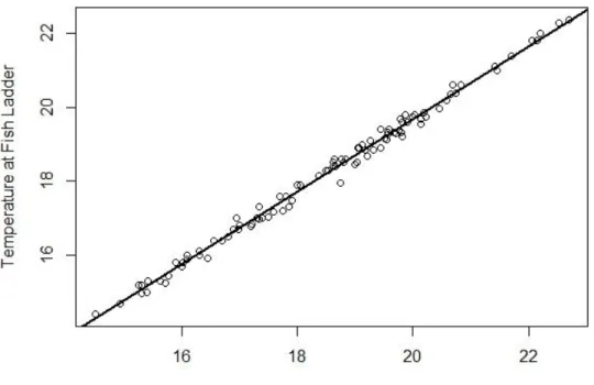
River temperature measured at the fish ladder was slightly less than temperature measured at the Joe Savard (Figure 1), which is to be expected, given that the temperature logger at Joe Savard is c. 7 km downstream of the fish ladder and river temperature generally increases with increasing distance downstream. The relationship between measured temperature at the fish ladder and at Joe Savard was linear (Figure 2) and given by Equation 1.

Equation 1. y = 0.9844x - 0.0065 (R2 _{= 0.9933, p < 2.2e-16)}

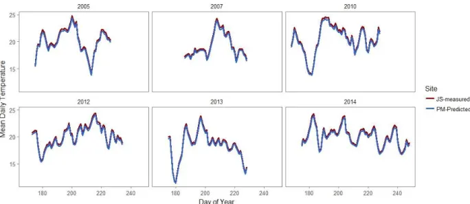
Assumptions of normality and homogeneity of variances were satisfied via visual examination of residual plots (Figure 3). Fish ladder temperatures estimated from river temperature measured at Joe Savard using Equation 1 are presented in Figure 4. We used the fish ladder temperature estimated for 2005, 2007, 2010, and 2012-2014 along with river temperature directly measured at the fish ladder during 2015 and 2016 in the analysis of fish ladder entry by migrating Atlantic salmon (Figure 5).

Figure 1. Temperature measured at the station Joe Savard (black line) and at the fish ladder (gray line) during summer 2015 (left) and 2016 (right).

4 Figure 2. Linear relationship between river temperature measured at JoeSavard and at the fish ladder during summer 2015 and 2016, given by the equation y = 0.9844x - 0.0065 (R2 = 0.9933, p < 2.2e-16).

Figure 3. Residual plots used to evaluate assumptions for the regression between river temperature measured at JoeSavard and measured at the fish ladder during the summers of 2015 and 2016.

5 Figure 4. River temperature measured at Joe Savard (red line) and river temperature estimated for the fish ladder from the equation y = 0.9844x - 0.0065 (R2 _{= 0.9933, p < 2.2e-16).}

Figure 5. River temperature at the fish ladder estimated from measured temperature at JoeSavard (first and second rows) and directly measured at the fish ladder (bottom row).

6

Discharge data were obtained from the Centre d’Expertise Hydrique Quebec (CEHQ) station 062803, located in the Sainte-Marguerite River Nord-Est, approximately 6 km downstream of the fish ladder. Fish counts from the Chute Blanche fish ladder were obtained from the MFFP. Whereas fish counts were available as daily totals only, river discharge and river temperature were logged at 15-min intervals. We therefore computed daily mean discharge and daily mean temperature prior to subsequent analyses.

2.3 Modeling Presence-Absence Data

Daily fish counts, mean daily temperature, and mean daily discharge were combined into one data table. A column designating each day as presence (salmon caught in fish ladder) or absence (no salmon caught) of fish at the fish ladder was added. In total, there were 136 days classified as “salmon absent” and 344 days classified as “salmon present” (Figure 6). The number of days with salmon absent was greater during the later years of the study (Figure 7). The number of absences recorded ranged from 8 to 35 days per year, whereas presences were recorded 34-60 days per year.

Figure 6. Distribution of “presence” and “absence” of salmon at the Chute Blanche fish ladder during the years when sufficient temperature data were recorded to permit assessment of the effects of temperature and discharge on fish capture (2005, 2007, 2010, and 2012-2016).

7 Figure 7. Number of “presences” (1) and “absences” (0) of salmon at the fish ladder for each year with sufficient temperature data to permit assessment of the effects of temperature and discharge on fish capture (2005, 2007, 2010, and 2012-2016).

Four logistic regression models were fitted to the complete dataset, where Tx was water temperature on day x, and Qx was river discharge on day x.

Model 1: log[ 𝑝(𝑦=1 ǀ𝑋) 1−𝑝(𝑦=1 ǀ 𝑋)] = 𝛽0+ 𝑇𝑥 Model 2: log[ 𝑝(𝑦=1 ǀ𝑋) 1−𝑝(𝑦=1 ǀ 𝑋)] = 𝛽0+ 𝑄𝑥 Model 3: log[ 𝑝(𝑦=1 ǀ𝑋) 1−𝑝(𝑦=1 ǀ 𝑋)] = 𝛽0+ 𝑇𝑥 + 𝑄𝑥 Model 4: log[ 𝑝(𝑦=1 ǀ𝑋) 1−𝑝(𝑦=1 ǀ 𝑋)] = 𝛽0+ 𝑇𝑥 + 𝑄𝑥 + 𝑇𝑥𝑄𝑥

Model fit was assessed using the Hosmer-Lemeshow statistic, which is more appropriate for assessing goodness of fit than use of the deviance statistic when the logistic model includes continuous independent variables (Kleimbaum and Klein 2010). Three measures were used to assess the discriminatory ability of each model: sensitivity, specificity, and the area under the receiver operating curve. Sensitivity reflects the ability of the model to correctly predict presence of fish (rate of true

8

positives) and specificity reflects the ability of the model to correctly predict true absence of fish (Hosmer et al. 2013). Specificity is used to generate the false positive rate, i.e., 1-specificity (Kleinbaum and Klein 2010). Plotting the true positive rate by the false positive rate generates the receiver operating curve (ROC). The area under the curve (AUC) indicates the ability of the model to predict true negative and true positives: an AUC equal to 1 indicates perfect discrimination (Kleimbaum and Klein 2010). Model selection was accomplished using analysis of deviance to compare nested models. The best model was that which significantly minimized residual deviance (Hosmer et al. 2013).

All analyses were conducted using R version 3.3.0 (R Core Team 2016) in R Studio version 1.0.136 (RStudio Team 2012). The Hosmer-Lemeshow goodness of fit test was performed using the package ResourceSelection (Subhash et al. 2016). Plots of ROC curves and the calculation of AUC were generated using the package ROCR (Sing et al. 2005). Graphics were created using ggplot2 (Wickham 2009).

2.4 Modeling Daily Count Data

We fitted generalized linear models for Gaussian, Poisson, negative binomial distributions, and generalized additive models to the data set, using the daily count of salmon entering the fish ladder as the response variable. For each type of model, we included the main effects of temperature, discharge, day of year, and year as predictors, and compared models using the Akaike information criterion (AIC). The general rule of thumb for comparing AIC scores is that if the AIC of two models differs by > 2, there is substantial evidence that the model with the lower AIC score is the better model. If AIC differs by > 10, then the model with the greater AIC score is very unlikely (Burnham and Anderson 2002). The function glm from the “stats” package was used to fit models using Gaussian, Poisson, and negative binomial distributions (R Core Team 2016). Generalized additive models were fitted using the package “mgcv” in R (Wood 2011).

9

3.

R

____________________________________________________________________________________

3.1 Modeling Presence-Absence Data

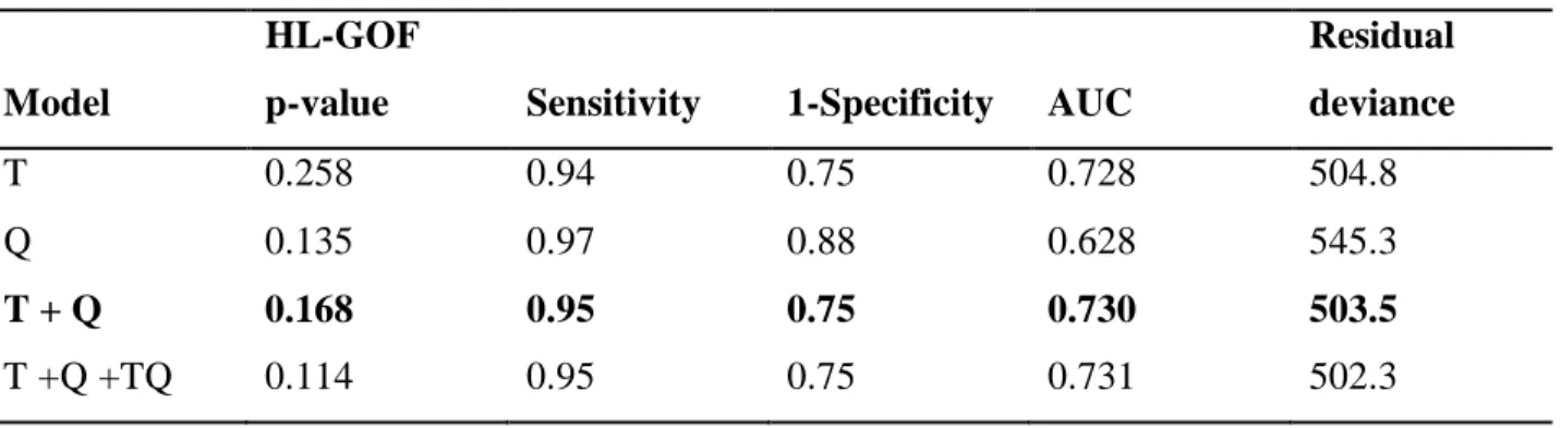
Based on the Hosmer-Lemeshow goodness of fit test, there was no evidence for lack of fit for any of the four logistic regression models fitted to the data (Table 1, p > 0.10). The area under the curve (AUC) was essentially equivalent (approximately 0.73) for all models that contained temperature as a covariate, indicating that the discriminatory ability of each model (i.e., the ability to correctly predict true presence and true absence of fish) was fair (Kleinbaum and Klein 2010). The model containing discharge as the sole covariate, however, had poor discriminatory ability (AUC < 0.7, Kleinbaum and Klein 2010). Including both temperature and discharge significantly reduced model deviance over the model with discharge alone (p = 1.016e-10). Addition of the interaction between temperature and discharge did not significantly reduce model deviance (p = 0.2799). The best model, therefore, included temperature and discharge as covariates. The false positive rate (1-specificity) was high for all models (≥ 0.75), which indicated that although the model did a good job of predicting true positives (sensitivity), it did not do a good job of predicting true negatives.

Table 1. Logistic regression models with goodness of fit statistics (Hosmer-Lemeshow, HL-GOF; sensitivity; false positive rate, presented as 1-specificity, and the area under the receiver operating curve, AUC) and model selection statistics (residual deviance). The best model, selected using analysis of deviance, is in bold.

Model

HL-GOF

p-value Sensitivity 1-Specificity AUC

Residual deviance T 0.258 0.94 0.75 0.728 504.8 Q 0.135 0.97 0.88 0.628 545.3 T + Q 0.168 0.95 0.75 0.730 503.5 T +Q +TQ 0.114 0.95 0.75 0.731 502.3

The high false positive rate was thought to result from the high number of presences (n = 344) relative to absences (n = 136) of fish in the fish ladder. We therefore subsampled the data such that the number of presences and absences were equal by randomly drawing (without replacement) 136 data points from among the presences, using the function sample_n in the dplyr package for R (Wickham and Francois 2016). We repeated this process 100 times and for each iteration applied a

10

logistic regression model and extracted model coefficients, residual and null deviance, Nagelkerke’s R2, the Hosmer-Lemeshow statistic, sensitivity, and specificity. We repeated this procedure two times; first with standardized predictors (by subtracting the mean and dividing by the standard deviation), and then with non-standardized predictors. Standardizing was used to ensure that we were not randomly drawing only extreme values of discharge or temperature. Because the initial analysis using the full dataset indicated that inclusion of both temperature and discharge improved the model fit, we only applied the bootstrap routine to models containing both temperature and discharge as predictors. Figure 9 summarized the outputs (coefficient and diagnostics) for the models A) Temperature + Discharge; and B) Temperature + Discharge + Interaction.

The 95% CI around the estimates of coefficients for both the model containing discharge and temperature and the model containing temperature, discharge, and the interaction are fairly narrow, indicating that the coefficients are stable and collinearity is not a problem for either model. The use of the subsampled data resulted in no improvement in Nagelkerke’s R2_{, sensitivity, or specificity}

compared with the models that used the full data set. We conclude, therefore, that use of the full dataset was appropriate for predicting the probability of a fish entering the fish ladder.

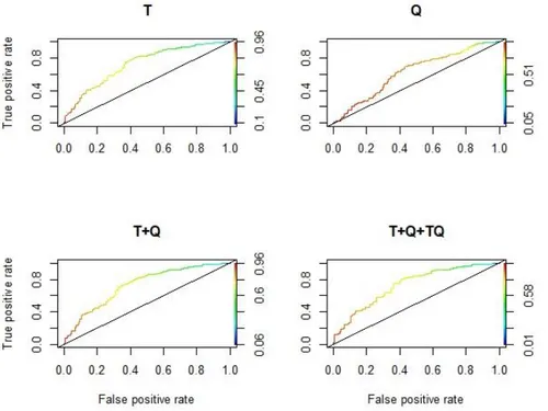
Figure 8. Receiver operating curves (ROCR) for the fitted logistic models with the covariates mean daily temperature (T, top left), mean daily discharge (Q, top right), temperature and discharge (T+Q, bottom left), and temperature, discharge, and the interaction term (T+Q+TQ, bottom right).

11 Figure 9. Distribution of bootstrap logistic regression model coefficients and diagnostics for the models A) T + Q and B) T + Q + TQ, where T is mean daily temperature and Q is mean daily discharge. Horizontal bars represent the median, hinges represent the 25th and 75th percentiles, and whiskers represent 1.5*IQR (inter-quartile range).

12

3.2 Modeling Count Data

Daily count data failed to meet the assumptions of normality and homogeneity of variances (determined by examining residual plots). Neither the application of data transformations nor standardizing succeeded in linearizing the data, thus the generalized linear model was inappropriate for predicting the relationship between river temperature, discharge, and the presence of fish in the fish ladder entry cage (as count data), and is reflected in the AIC values obtained, which are substantially greater than those obtained via the negative-binomial method.

The count data at the fish ladder were found to suffer from dispersion. Data are considered over-dispersed if the variance is greater than the mean, which is commonly observed in count data. In the case of the fish ladder, the mean count was 3.5 salmon/day, whereas the variance was 25.0. Both Poisson regression and negative-binomial regression can be applied to over-dispersed data. The models fit with the Poisson distribution had AIC values that were much greater than those obtained by the Gaussian or Negative-Binomial distributions, therefore, the Poisson regression could be ruled out as providing an appropriate fit to the data. This is likely because the degree of over-dispersion in the fish ladder count data was too great to be resolved with the use of the Poisson distribution.

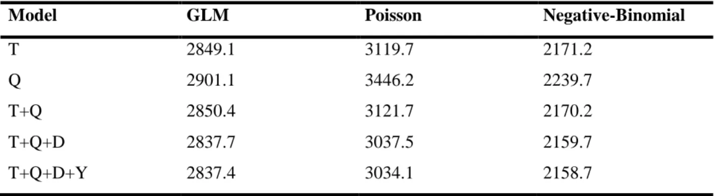
Table 2. Akaike information criterion for models fitted using the Gaussian (GLM), Poisson, and negative-binomial distributions. Predictive variables included in each model were mean daily river temperature (T), mean daily river discharge (Q), day of year (D), and Year (Y).

Model GLM Poisson Negative-Binomial

T 2849.1 3119.7 2171.2

Q 2901.1 3446.2 2239.7

T+Q 2850.4 3121.7 2170.2

T+Q+D 2837.7 3037.5 2159.7

T+Q+D+Y 2837.4 3034.1 2158.7

Among the three classes of models, those fit to the count data using the negative binomial distribution had the lowest values of AIC, with the model that included temperature, discharge, day, and year obtaining the lowest value of AIC. The addition of year did not substantially reduce AIC relative to

13

the model that included temperature, discharge, and day (Δ < 2), indicating that neither model had more support than the other. Consequently, we examined goodness of fit criteria (Nash coefficient, RMSE, and bias) for the models T + Q + Day + Year and T + Q + Day. Both models had a Nash coefficient < 0.1 and RMSE of nearly 100%, indicating that the models had almost no predictive capability. An example of these goodness of fit criteria is shown for the model T + Q + Day of Year + Year (Table 3). Because of the low predictive power of these models, we did not attempt to include interactions along with the main effects, as is was thought they would not substantially improve model fit.

Table 3. Mean fish count per day, RMSE, Nash coefficient, and bias for each year for the negative binomial model: Number of salmon = T + Q + Day of Year + Year.

As the data were not adequately modelled using a linear framework, we attempted to apply a generalized additive model (GAM) to the relationship between fish count and the previously described environmental variables (mean daily temperature, mean daily discharge, day, and year). We applied the GAM to the raw data, as well to data standardized using Z-scores. Z-scores were calculated for the fish counts, temperature, and discharge.Using the raw data, the AIC score for the model T + Q + Day + Year was 2770.0, which was much greater than the model fitted using the negative-binomial distribution (ΔAIC >10), indicating that the GAM model was less likely than the model fitted using the negative-binomial (Burnham and Anderson 2002). We cannot compare the AIC scores between models fitted using the raw count data and models fitted with the Z-score standardized data, because the response variable must be the same across models. The model T + Q

Year RMSE Nash Bias 2005 4.10 4.89 -0.05 0.62 2007 3.14 3.71 0.05 0.03 2010 6.10 7.11 0.07 -1.12 2012 4.76 7.20 -0.09 -0.79 2013 3.57 4.01 0.37 -0.88 2014 2.00 3.73 -0.68 2.43 2015 1.33 2.00 -0.40 0.94 2016 3.27 3.19 0.04 -0.85 2013 3.57 4.01 0.37 -0.88 2014 2.00 3.73 -0.68 2.43 2015 1.33 2.00 -0.40 0.94 2016 3.27 3.19 0.04 -0.85 Mean Count

14

+ Day received an AIC score of 1261.9. The Nash coefficient was 0.11 and the RMSE was 0.93. Consequently, the use of the GAM with standardized count data also resulted in poor predictive power.

4.

C

____________________________________________________________________________________

We applied three main modelling approaches (logistic regression, GLM, and GAM) to examine the effect of river temperature and discharge on attractivity of the fish ladder at Chute Blanche on the Nord-Est Sainte Marguerite River. The approach that best predicted the relationship between fish ladder attractivity and environmental variables was the logistic model. Generalized linear models using Gaussian, Poisson, and negative binomial distributions were found to have poor fit to the data and had low predictive power for modelling the relationship between the number of salmon entering the fish ladder daily at Chute Blanche and environmental variables (mean daily temperature, mean daily discharge, day of year, and year). Generalized additive modelling was also found to have poor predictive power.

The logistic regression model that best predicted the probability of a salmon entering the fish ladder included mean daily temperature (T) and mean daily discharge (Q; Equation 2). The coefficient estimates provide us with the change in the log odds with a one-unit increase in the predictor variable (Table 2). The temperature coefficient estimated by the model was 0.378 and the discharge coefficient was -0.012. This means that for every one unit change in temperature, the log odds of fish (versus no fish) increases by 0.378, and for every 1 unit change in discharge, the log odds of fish (versus no fish) decreases by 0.012.

Equation 2. 𝑝(𝑦 = 1|𝑋) = exp (−6.0 + 0.378𝑇−0.012𝑄)

15 Table 4. Coefficients for the logistic regression model log[ 𝑝(𝑦=1 ǀ𝑋)

1−𝑝(𝑦=1 ǀ 𝑋)] = 𝛽0+ 𝑇𝑥 + 𝑄𝑥, where T =

temperature and Q = discharge, with associated standard error and p-values.

Coefficient Estimate Standard Error Z-value Pr(>|z|)

Intercept -6.00883 1.27562 -4.711 2.47e-06

Temperature (T) 0.37837 0.06249 6.055 1.40e-09

Discharge (Q) -0.01164 0.01047 -1.111 0.266

The log odds are used to obtain estimates of the odds, which is the outcome of interest, because the odds provide an estimate of the probability of an event occurring; in our case, the probability of a salmon entering the fish ladder given temperature and discharge. Log odds are the natural logarithm of the odds, thus to obtain the odds, we take the natural exponent of the coefficients. For a one-unit increase in temperature, the odds of salmon entering the fish ladder (versus not entering) increases by a factor of 1.5, over the temperature range observed (11-24◦C). That means that a salmon is 1.5 times more likely to enter the fish ladder at 19◦C than at 18◦C. A one-unit increase in discharge (i.e. an increase of 1 m3s-1) is not particularly interesting, but a 10-unit increase in discharge is: for a 10-unit increase in discharge (i.e., if discharge increases by 10 m3s-1), the odds of a salmon entering the fish ladder is 0.89. In other words, for a given temperature, if river discharge increases by 10 m3s-1, a salmon is less likely to enter the fish ladder. If river discharge decreases by 10 m3s-1, however, a salmon is 1.12 times more likely to enter the fish ladder. If river discharge decreases by 20 m3s-1, a salmon is 1.26 times more likely to enter the fish ladder.

In conclusion, salmon were more likely to enter the fish ladder at lower discharge for the range of temperatures encountered during the study years (Table 5). Salmon were more likely to enter the fish ladder at greater discharge when water temperature was warm. For example, at river discharge of 10 m3_s-1_{, the probability of a salmon entering the fish ladder when river temperature was 14}◦_{C was only}

0.30, whereas at 22◦C, the probability of a salmon entering the fish ladder was 0.90, and the probability of a fish entering the fish ladder at 10 m3_s-1 _{and 18}◦_{C was approximately the same as the}

16 Table 5. Probability of a salmon entering the fish ladder at Chute Blanche for varying levels of temperature and discharge.

Although the false positive rate associated with the final model was greater than we would have hoped, the AUC of 0.73 indicated that the discriminatory ability of the model (i.e., the ability to correctly predict true presence and true absence of fish) was adequate (Kleinbaum and Klein 2010). Temperature data were only available for eight of the thirteen years for which we had discharge and fish count data, thus we had to eliminate seven years of data from our analysis. Had we been able to include all thirteen years of data, it may have been possible to obtain a model with greater discriminatory ability. A generalized additive model exists to model river temperature from air temperature and discharge, however, we were unable to use this model to generate river temperature estimates to fill out our data set, as we wished to disentangle the effects of river temperature and discharge on the probability of fish entering the fish ladder. As river temperature models become available for the Nord-Est Sainte Marguerite River that do not rely on discharge, it will become possible to repeat this logistic regression analysis with all years included in the dataset, which may improve the discriminatory ability of the model.

5.

A

____________________________________________________________________________________

This work was supported by the Fédération Québécoise du Saumon Atlantique. Additonal financial support for D. Frechette was provided by the Fonds de recherche du Québec - Nature et technologies (FRQNT) Merit Scholarship Program for Foreign Students. We would like to thank the Ministere de la Faune, des Fôrets, et des Parcs du Québec for access to river temperature and fish count data, and

14◦C 18◦C 19◦C 22◦C 10 0.30 0.66 0.74 0.90 20 0.28 0.64 0.72 0.89 30 0.26 0.61 0.70 0.88 40 0.24 0.58 0.67 0.86 60 0.20 0.53 0.62 0.83 80 0.16 0.47 0.56 0.80 Probability of Entry Discharge (m3s-1)

17

C. Boyer for providing access to the RivTemp data set. We also thank the Association de la Rivière Sainte-Marguerite and the Corporation de Pêche Ste-Marguerite for their collaboration and support of this research, and all the operators who diligently recorded data at the Chute Blanche fish ladder. In particular, we wish to thank K. Gagnon, S. Gravel, M. Murdock, V. Maltais, P. Rousseau, and M. Valentine.

6.

R

____________________________________________________________________________________

Hosmer Jr, D.W., Lemeshow, S. and Sturdivant, R.X. (2013). Applied Logistic Regression 3rd ed. John Wiley & Sons, Inc., Hoboken, New Jersey

Kleinbaum, D.G., and Klein, M. (2005). Survival Analysis: A Self-Learning Text. 2 edition. Springer. RStudio Team (2012). RStudio: Integrated Development for R. RStudio, Inc., Boston, MA

URL http://www.rstudio.com/.

R Core Team (2016). R: A Language and Environment for Statistical Computing. R Foundation for Statistical Computing. Vienna, Austria. https://www.R-project.org.

Subhash R. Lele, Jonah L. Keim and Peter Solymos (2016). ResourceSelection: Resource Selection (Probability) Functions for Use-Availability Data. R package version 0.3-0.

https://CRAN.R-project.org/package=ResourceSelection

Wickham, H. (2009). ggplot2: Elegant Graphics for Data Analysis. Springer-Verlag New York. Wickham, H. and Francois, R. (2016). dplyr: A Grammar of Data Manipulation. R

package version 0.5.0. https://CRAN.R-project.org/package=dplyr Wood, S.N. (2011) Fast stable restricted maximum likelihood and marginal

likelihood estimation of semiparametric generalized linear models. Journal of the Royal Statistical Society (B) 73(1):3-36