To cite this document:
Boco, Hervé and Germain, Laurent and Rousseau, Fabrice
When overconfident traders meet feedback traders. (2011) In: Midwest Finance
Association Annual Meeting, 3-6 Mar 2011, Chicago, United States.
O
pen
A
rchive
T
oulouse
A
rchive
O
uverte (
OATAO
)
OATAO is an open access repository that collects the work of Toulouse researchers and makes it freely available over the web where possible.
This is an author-deposited version published in: http://oatao.univ-toulouse.fr/
Eprints ID: 5794
Any correspondence concerning this service should be sent to the repository administrator: [email protected]
When Overconfident Traders Meet Feedback Traders.
Hervé Boco, Laurent Germain and Fabrice Rousseau
April 2010
Abstract
In this paper, we develop a model in which overconfident market participants and rational speculators trade against trend-chasers. We exhibit the unique linear equilibrium and assess the quality of prices according to the proportion of the different types of agents. We high-light how speculative bubbles arise when a large number of traders adopt a trend-chasing behavior. We show that overconfident traders can obtain positive expected profits. In par-ticular, overconfident traders can outperform rational traders. The positive feedback trading enhances the negative correlation between the back-to-back prices changes and the volatil-ity of prices as well. We show that positive feedback traders destabilize prices more than their overconfident opponents. Generally, overconfidence increases the volatility of prices and worsens the market efficiency. But, we show that in the presence of positive feedback trading, overconfidence improves the market efficiency and dampens the excess volatility.
Keywords: Overconfidence, Positive feedback trading, Bubbles, Excess volatility, Market efficiency.
Introduction
Most financial studies assume market efficiency and consider that agents behave rationally. In doing so, they fail to explain some properties observed in financial markets such as booms and crashes (Kunieda (2007), Kaizoji (2000)); the underreaction or overreaction of market partic-ipants (De Bondt and Thaler (1985, 1987, 1990), Daniel et al. (1998)); the excessive volume traded (Dow and Gorton (1997), Odean (1998)). Behavioral finance has emerged primarily to explain these anomalies. Among all the psychological biases and forms of irrationality, two psy-chological traits of market participants have been widely investigated: the overconfidence and the trend-chasing behavior.
In this paper we exhibit a mpodel where the bubble crashes emerge from the presence of irrational tarders in a dynamic setting. Irrationality is modeled through overconfidence and feedback trading.
However, according to Fama (1965, 1970), there are enough informed traders and well-financed arbitrageurs present in the market to guarantee that any potential mispricing induced by behavioral traders is corrected at a certain point. Therefore, the efficiency theory rules out the persistence and even the presence of bubbles. Nevertheless, many bubbles and crashes examples can be found. The most famous one is undoubtedly the Dutch Tulip Mania, which occurred in 1630. This was the first derivatives market crash. Some other famous crashes include the Mississippi Bubble in 1721, the Asian market collapse in 1997, the Russian monetary system bankruptcy in 1998 and more recently the dot-com bubble crash in 2001 as well as the subprime crisis and the “credit crunch”, which began during the summer 2007.
The purpose of this paper is to study the interaction between overconfident and feedback traders (momentum as well as contrarian traders) and how this interaction may trigger the creation of bubbles and their subsequent crash. Indeed, positive feedback or momentum traders buy (sell) securities when prices rise (fall). In doing so, they introduce noise into the market since they lead prices to move away from fundamentals. However, negative feedback or contrarian traders sell (buy) securities when prices rise (fall). This behavior limits the movement of prices. To study such a situation, we use the dynamic model of De Long et al. (1990). We in-troduce the presence of informed overconfident traders in their model in order to look at how
overconfident traders exploit the presence of feedback traders.1 When positive feedback traders
are present, informed traders stimulate trading by positive feedback investors, by trading, early, large quantities and therefore building up a large position. In the last period, they off-load part of their position by going against their information. For the case of negative feedback trading, informed investors ???(we have to look at the simulations from the price behavior, I think that
1As in Germain et al. (2009), we consider that overconfident traders overestimate the mean of the liquidation
the price should gradually increase, but at a lower speed than if there were no negative feedback). We show that the growth and the burst of a financial bubble stem mainly from positive feedback trading and that overconfident informed investors are not responsible for its formation. However, we find that the presence of overconfident traders and the risk aversion of the informed speculators only enhance the strength of bubbles (creation and burst). This last result is in contrast to Figlewski (1979), Campbell and Kyle (1988). Indeed, we obtain that the informed traders’ risk aversion (for both the rational and the overconfident traders) does not dampen the fluctuation of the price schedule by keeping informed investors from taking large position.
This should be completed with the negative feedback if there is anything to say concerning bubbles which I doubt.
Our analysis, apart from shedding some light on the emergence and the burst of bubbles, will also enable us to answer the following important questions. What is the main determinant of the excess price volatility? How does the link between psychological characteristics of the participants and their trading profits evolve according to different proportions of irrational traders? What is the effect of the traders’ risk aversion on price stabilization? Where do the underreaction and/or overreaction to new information come from?
We first give our results for the case where there is no feedback trading (Do we need to put that, as there is not much difference with existing results). In that case, the trading of overconfident investors enhances the volatility of prices, and worsens the quality of prices as well as their expected profits.We obtain that the presence of overconfident implies larger volume traded. In addition, we find that the trading volume increases as the mean bias increases. Statman, Thorley, and Vorkink (2006) use U.S. market level data to test the former effect and argue that after high returns subsequent trading volume will be higher as investment success increases the degree of overconfidence.
Our second set of results looks at the case where feedback traders are present. When there is a sufficient large number of trend-chasing speculators, overconfident traders may earn more profits than their rational opponents. In addition, overconfidence diminishes the volatility of prices (whereas momentum trading always enhances it), and increases market efficiency (momentum trading worsens it). We obtain that asset returns are negatively serially correlated. Daniel, Hirshleifer and Subrahmanyam (1998) consider a situation where investors are overconfident about the precision of their private signals. However, the noisy public information is correctly estimated by all market participants. They then exhibit a positive short-lag autocorrelations (that they call the “overreaction phase”) and a negative correlation between future returns and long-term past stock market (the long-run reversals that they call the “correction phase”). Finally, when positive feedback traders are present we obtain both rational and overconfident traders trade more. Moreover, positive feedback traders earn negative expected profits.
When we look at negative feedback, we find that most of the results obtained with the presence of positive feedback are reversed. Price volatility is reduced whereas price efficiency is enhanced due to the presence of contrarian trading. Price volatility and price efficiency increase with both the number of overconfident traders and with their level of overconfidence. The overall volume traded by rational traders increase with the number of negative feedback whereas the volume traded by overconfident is U -shaped with respect to the number of negative feedback. We find the serial correlation of returns to be negative and to decrease with the number of negative feedback. Finally the expected profit of the negative feedback traders decrease with the number of negative feedback traders present in the market and is positive for low enough number of negative feedback traders.
The trend-chasing behavior has been shown to exist both experimentally and empirically. Andreassen and Kraus (1990) and Mardyla and Wada (2009) use experiments to show its exis-tence. Andreassen and Kraus (1990) show that over a period prices exhibit a trend relative to the period variability, subjects chase the trend, buying more when prices rise and selling when prices fall. However, this phenomenon occurs only as a response to significant changes in the price level over a substantial number of observations and not in response to the recent price changes alone. Mardyla and Wada (2009) investigate a virtual stock market to understand the link between public information and short-term investment behavior at the individual decision-making level. They distinguish between three types of public information: prices movements, macroeconomic news and relevant individual-stock information. They find that for 75% of the cases, the subjects adopt positive feedback strategies.
In addition, other analysis have empirically found evidences of trend-chasing behavior in finan-cial markets. Frankel and Froot (1988) observe that in the mid-1980’s the forecasting services were issuing buy recommendations while maintaining that the dollar was overpriced relative to its fundamental value. Lakonishok, Shleifer and Vishny (1994) find evidences that individual investors use positive feedback trading strategies and that this behavior can be attributed to an irrational extrapolation of past growth rates. Several studies have focused on the behavior of institutional investors (Shu (2009), Sias and Starks (1997), Sias, Starks and Titman (2001), Den-nis and Strickland (2002) to name but a few). According to most of these papers, institutional investors use positive feedback strategies and therefore destabilize stock prices. Finally, Bohl and Siklos (2005) find the existence of momentum strategies during episodes of stock market crashes. Evidences of contrarian strategies are also present in financial markets. The short-term portfolio composition strategies suggested by Conrad et al. (1994), Cooper (1999), and Ger-vais et al. (2001) found that US markets showed anomalous, “contrarian” behavior. Moreover, Evans and Lyons (2003) obtain evidence of negative feedback trading, at the daily frequency. This literature concludes that the presence positive (negative) feedback traders leads to negative (positive) serially correlated returns together with an increase (decrease) in volatility.
The overconfidence was firstly analyzed by psychologists. Kahneman and Tversky (1973), and Grether (1980) stress that people overweight salient information. This behavior is well documented in psychology for very diverse situations. Due to the essence of financial markets, overconfidence occurs among market participants. Indeed, the competition between traders leads the most successful ones to survive, leading them to overestimate their own ability.
Many academic papers have looked at the impact of overconfidence on financial markets. Most of the studies predict that overconfident agents trade to their disadvantage (Odean (1998), Gervais and Odean (2001), Caballé and Sákovics (2003), Biais et al. (2004) among others). In contrast, Kyle and Wang (1997), Benos (1998) and Germain et al. (2009) find that overconfident traders can have larger expected profit than their rational counterpart. The other most cited effect of the presence of overconfident traders is a large trading volume (Odean (1998), Barber and Odean (2001) among others).
Hirshleifer, Subrahmanyam and Titman (2006) show that irrational traders can earn positive expected profit in the presence of positive feedback trading if they trade early. Indeed, higher stock prices may attract customers and employees which may reduce the firm’s cost of capital and provide a cheap currency for making acquisition. Also, stock prices increase may initially
generate cash flow.2 This simple mechanism does not require irrational traders to be
sophisti-cated enough to think of the positive feedback trading effect and to realize profits. In contrast to Hirshleifer et al. (2006), we do not consider a direct link between the stock prices and the corresponding firm’s output which might be embodied by the means of positive feedback trading. Such a link is considered through the information which is observed by informed traders.
The outline of this paper is as follows. In section 2, we introduce the general model and characterize the different types of traders. In section 3, we derive the trading equilibrium. In section 4 we analyze the effects of the overconfidence and of the feedback trading on the variances of prices. In section 5, we are interested in understanding the social standpoint. In section 6, we discuss our results in terms of the range of parameters. In section 7, we look at how our results are changed when we replace positive feedback traders by negative feedback tarders. Finally, we conclude in section 7. All proofs are gathered in the Appendix.
1
The Model
We consider a model with a three-period auction. Two assets, namely a riskless and a risky asset, are exchanged at t = 1, 2, 3. The riskless interest rate is normalized to zero. The
liquidation value of the risky asset, ˜v, is assumed to be normally distributed with ˜v ∼ N(¯v, h−1
v ).
2
It is straightforward that dot-com economy has benefited from this advantage by attracting the best students from top programs such as Standford University and by raising large funds (see Fortune "MBAs Get Dot.com Fever" August 2 1999).
Consumption takes place at the end of the game, i.e. at t = 4.
We consider a trading system where agents are price takers. At each auction t, the demands for
the risky asset and the riskless asset are xt and ft respectively. Three types of investors trade
the assets:
• N1 overconfident traders. They receive information about the liquidation value of the risky
asset. They believe that their private signals are more accurate than they actually are. Furthermore, they overestimate the expected liquidation value of the risky asset.
• N2 rational traders. These traders receive private information but do not distort it.
• P feedback agents who can either be positive feedback or negative feedback traders. Their order size is proportional to the variation of the price of the asset.
We denote by Pt the price of the risky asset at time t for t = 1, 2, 3. At time t = 4, the value
of the risky asset is publicly revealed, the price is then equal to the realization of ˜v.
Trader i’s wealth is Wti= fti+ Ptxti for trading rounds t = 1, 2, 3 and W4i= f3i+ ˜vx3i for the
last trading round. Let us denote ¯x as the per capita supply of the risky asset. It is assumed to
be known to all and constant over time.
No information is released before the first trading round. Before each subsequent trading round t = 2 and t = 3, each rational or overconfident trader receives one of M different signals
concerning the liquidation value of the asset. We have that M < N1+ N2. Each trader receives
a private signal ˜yti= ˜v + ˜εtm, with ˜εtm∼ N(0, h−1ε ) and ˜εt1, . . . , ˜εtmfor ∀ t = 1, 2, 3 are mutually
independent. Let ¯Yt be the average private signal at time t, we assume that:
¯ Yt= M X i=1 ˜ yti M = N1 X i=1 ˜ yti N1 = N2 X i=1 ˜ yti N2
in other words, the informativeness of the private signals is the same for the two groups. Overconfident market participants believe that the precision of their two signals, the one received
at t = 2 and the other received at t = 3, is equal to κhε with κ ≥ 1. They also believe that the
2M −2 other signals have a precision equal to γhεwith γ ≤ 1. Overconfident traders misperceive
the distribution of the asset as well. Indeed, they believe that the average liquidation value equals ¯
v + b with b > 0 and that the precision of ˜v equals ηhv (η ≤ 1).3 This framework is consistent
with theoretical and empirical findings. Indeed, traders tend to overestimate their own signals and to correctly evaluate (or at worst to under-weight) public information.
A rational agent correctly estimates both the mean of the liquidation value of the risky asset
and her private signal. In other words, a rational investor acts as an optimistic trader with η = κ = γ = 1 and b = 0.
For simplification we assume that both N1 and N2 are multiple of M . This assumption
leads to the fact that optimistic traders are, on average, equally informed as their rational counterparts. This setup allows us to exhibit the overconfidence effect without considering informational content bias.
All informed agents are assumed to be risk averse. Their preferences are described by a constant absolute risk aversion (CARA) utility function of the following form
u(W ) = −e−aW
where a denotes the coefficient of risk-aversion and W the wealth.
Each informed trader i chooses his order at time t, xti, so that
xti∈ arg max E[−e−aWti|Φti],
where Φti denotes the information available to them.
As in Odean (1998), informed traders look one period ahead when solving for their optimal strategy.
Finally, at time t = 2, 3, each feedback positive agent i submits an order xfti, with :
xfti= β(Pt−1− Pt−2)
2
The equilibrium
To solve their maximization problems, informed traders whether rational or overconfident assume that prices are linear functions of the average signal(s) such that:
P3= α31+ α32Y¯2+ α33Y¯3, (2.1)
P2= α21+ α22Y¯2. (2.2)
At each auction, an informed agent determines his demand by considering both his pri-vate signal(s) and the price schedule(s). Each informed market participant i has access to the
following information Φ2i = [y2i, P2]T and Φ3i = [y2i, y3i, P2, P3]T for date t = 2 and t = 3,
respectively. Due to the presence of positive feedback trading, when deciding his demand, an informed trader takes into account that his trade may lead prices away from fundamentals. The positive feedback traders only participate to the last two rounds of trading. We now present the first proposition.
Proposition 2.1 There exists a unique linear equilibrium in the multi-auction market charac-terized by: α31 = (N(N11η+Nη+N22)h)hvv+2(Nv+N¯ 11ηh(κ+γM−γ)+Nvb−a(N1+N22+P )¯M )hxε + (N1η+N2)hv+2(NaP β1(κ+γM −γ)+N2M )hε(α21− P1) α32 = α33+(N aβP 1η+N2)hv+2(N1(κ+γM−γ)+N2M )hεα22 α33 = (N N1(κ+γM −γ)hε+N2M hε 1η+N2)hv+2(N1(κ+γM−γ)+N2M )hε
where α21, α22 and the different agents’ demands over time are given in the Appendix.
Proof: See Appendix.
The number of positive feedback traders has an impact on the different parameters α except on
α33. Indeed, at the last auction, informed agents cannot trigger feedback trading on the basis
of their new information. Nevertheless, all prices are impacted and connected by the presence
of trend-chasing traders. More precisely, the link between P3 and ¯Y2 (captured by α32) depends
on the link between P2 and ¯Y2 (i.e. α22). The greater the intensity of feedback trading (β and
P ) the stronger is this link. Similarly, the informed traders’ risk aversion, a, strengthens this link.
In our model, as the both types of informed traders are aware of the presence of positive feedback traders, they take that into account when trading. Indeed, upon receiving good news before both t = 2 and t = 3 for instance, informed traders take larger position based on that information at t = 2 in order to drive prices up. This triggers even more buying subsequently from feedback traders which enables them to off load their position at an inflated price resulting in positive expected profit.
Odean (1998) is a particular case of our model and can be retrieved by setting, in our model,
the value of P , N2 and b to 0. He focuses on the resulting variance of prices, trading volume
and market efficiency when overconfident traders are present in the market.
In contrast to us, in Hirshleifer et al. (2006) irrational traders do not anticipate the feedback effect. Moreover, in their model, the rise in price causes stakeholders (for instance workers) to make greater firm-specific investments when they anticipate the growth of the firm. This in turn increases the final payoff of the risky asset. This explains why risk aversion cannot lead price to be negative and has no impact on the existence of a stock market equilibrium. Nevertheless, risk averse traders trade less aggressively and dampen the feedback effect.
3
Volatility, Quality of Prices, Serial Correlation of prices and
Trading Volume
In this section, we focus on the influence of the irrational behavior on the volatility of prices, measured as the variance of prices, on the quality of prices at t (the variance of the difference
between the price and the liquidation value, var(Pt− ˜v)), the serial correlation of prices and on
the different market participants’ trading volume.
3.1
Volatility
Proposition 3.2 The variance of prices, for both trading rounds t = 2, 3, increases with the
number of positive feedback traders. In the presence of trend-chasing behavior, the overconfidence can diminish the volatility of prices.
Proof: See Appendix.
The first part of the proposition implies that in the presence of positive feedback traders, neither rational informed agents nor overconfident informed traders can stabilize stock prices as they exploit the presence of feedback traders. This result is consistent with De long et al. (1990). However, numerous previous studies have pointed out that the excess volatility of asset prices stems from the trading behavior of overconfidence traders (Odean (1998), Caballé and Sákovics (2000), among others). We find that excess volatility depends critically on the number of feed-back traders in the market. When there are no positive feedfeed-back, we obtain the aforementioned result of Odean (1998) and Caballé and Sákovics (2000). However, when there are positive feedback traders present this result can be reversed. We find that the main source of excess volatility is due to feedback trading rather than the trading from overconfident traders. Hence, overconfident traders can alleviate the effect of the feedback trades and lead to a more stable market.This can be explained as follows, when changing the number of informed traders, the following forces are at work. Increasing the number of informed traders (both rational and overconfident) on the one hand stabilizes prices as it increases the risk bearing capacity of the market. On the other hand it destabilizes prices as more traders anticipate the trend-chasing behaviour. The more positive feedback traders in the market, the larger the latter effect. The combination of the two effects lead to the comparative statics below.
Some other studies, such as Hilton (2000), Glaser, Nöth and Weber (2004), De Bondt (1998), Graham and Harvey (2003), have found a similar result. However, all these studies investigate only one type of irrational trading. In contrast to these papers, we look at different types of irrational traders.
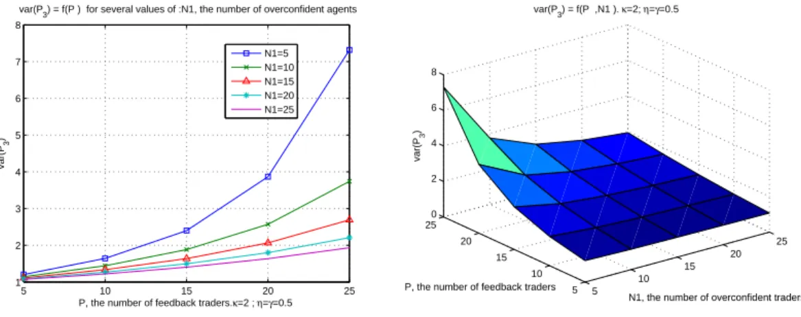
The figures below show the volatility of prices for different parameters of our model.
In figure 1, we obtain that the volatility of prices increases with the number of positive feedback traders and decreases with the number of overconfident agents.
5 10 15 20 25 1 2 3 4 5 6 7 8
P, the number of feedback traders. κ=2 ; η=γ=0.5
var(P
3
)
var(P3) = f(P ) for several values of :N1, the number of overconfident agents N1=5 N1=10 N1=15 N1=20 N1=25 5 10 15 20 25 5 10 15 20 25 0 2 4 6 8
N1, the number of overconfident traders var(P3) = f(P ,N1 ). κ=2; η=γ=0.5
P, the number of feedback traders
var(P
3
)
Figure 1: The variance of prices at time t = 3 as a function of the number of feedback traders and of
the number of overconfident traders.
In figure 2, we observe that the variance of prices increases when overconfident traders
underestimate the precision of the liquidation value of the risky asset (ηhv, with η ≤ 1). The
volatility of prices also increases when each overconfident agent believes the other (2M − 2)
signals to be γhε, with γ ≤ 1. The smaller the two parameters (η, γ), the greater is the
volatility of prices. This result is consistent with Odean (1998) and shows that underestimating the ability of other market participants causes the price setting to be destabilized.
5 10 15 20 25 1 1.5 2 2.5 3 3.5 4 4.5 5
P, the number of feedback traders. N1=N2=10 ; κ=2 ; η=0.5 var(P3) = f(P ) for several values of gamma
gamma=0.2 gamma=0.4 gamma=0.6 gamma=0.8 gamma=1 5 10 15 20 25 1 1.5 2 2.5 3 3.5 4 4.5
P, the number of feedback traders. N1=N2=10 ; κ=2 ; γ=0.5
var(P
3
)
var(P3) = f(P ) for several values of :eta
eta=0.2 eta=0.4 eta=0.6 eta=0.8 eta=1
Figure 2: The variance of prices at time t = 3 as a function of the number of γ and of η.
Figure 3 shows that as overconfident traders become more overconfident the volatility of prices decreases when trend chasing traders are present in the market.
5 10 15 20 25 1 1.5 2 2.5 3 3.5 4 4.5 5
P, the number of feedback traders. N1=N2=10 ; η=γ=0.5
var(P
3
)
var(P3) = f(P ) for several values of :kappa
kappa=1 kappa=2 kappa=3 kappa=4 kappa=5 5 10 15 20 25 1.1 1.2 1.3 1.4 1.5 1.6 1.7 1.8 1.9
N1, the number of overconfident agents. P=10 ; η=γ=0.5
var(P
3
)
var(P3) = f(N1 ) for several values of :kappa kappa=1 kappa=2 kappa=3 kappa=4 kappa=5
Figure 3: The variance of prices at time t = 3 as a function of the number of feedback traders and of
the number of overconfident traders.
In figure 4, we find that, without trend-chasing behavior, overestimating its own ability enhances the volatility of prices. The last graph shows that for intermediate values of P , the number of positive feedback traders, the volatility of prices decreases with the number of over-confident and is non-monotonic with the level of overconfidence.
5 10 15 20 25 0.91 0.92 0.93 0.94 0.95 0.96 0.97 0.98 0.99 1
N1, the number of overconfident agents. P=0 ; η=γ=0.5
var(P
3
)
var(P3) = f(N1 ) for several values of :kappa kappa=1 kappa=2 kappa=3 kappa=4 kappa=5 5 10 15 20 25 1.06 1.08 1.1 1.12 1.14 1.16 1.18 1.2 1.22
N1, the number of overconfident agents. P=5 ; η=γ=0.5
var(P
3
)
var(P3) = f(N1 ) for several values of :kappa kappa=1 kappa=2 kappa=3 kappa=4 kappa=5
Figure 4: The variance of prices at time t = 3 as a function of the number of feedback traders and of
the number of overconfident traders.
We now turn to the quality of prices.
3.2
Quality of Prices
In that subsection we examine the behavior of the quality of prices.
When the number of positive feedback traders increases, prices move away from fundamentals and therefore become less informative. Moreover, as informed traders anticipate the trend-chasing strategies they purchase ahead of feedback demand. As a consequence, the price quality worsens even more.
In addition to responding to the trend-chasing strategies, overconfident traders alter the
quality of prices due to their irrationality.4 Nevertheless, we can observe that the overconfidence
improves market efficiency when there is positive feedback trading (see the figures below). If there is no trend-chasing behavior, the presence of overconfident traders moves prices away from fundamentals and diminishes the market efficiency.
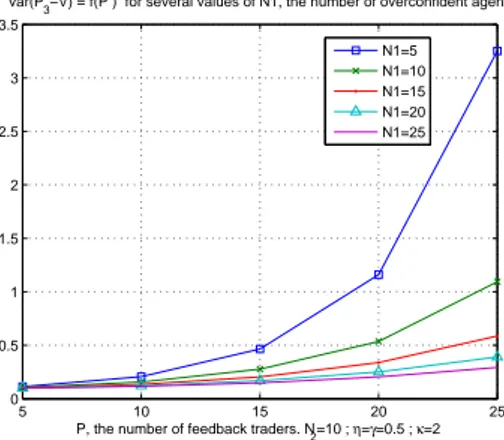
Figures 5 and 6 show that the quality of prices decreases with the number of positive feedback traders. For a fixed number of positive feedback traders, market efficiency increases with the number of overconfident traders and the parameter κ.
5 10 15 20 25 0 0.5 1 1.5 2 2.5 3 3.5
P, the number of feedback traders. N2=10 ; η=γ=0.5 ; κ=2 var(P3−V) = f(P ) for several values of N1, the number of overconfident agents
N1=5 N1=10 N1=15 N1=20 N1=25
Figure 5: The quality of prices at time t = 2 and t = 3 as a function of the number of feedback traders
and of the number of overconfident traders.
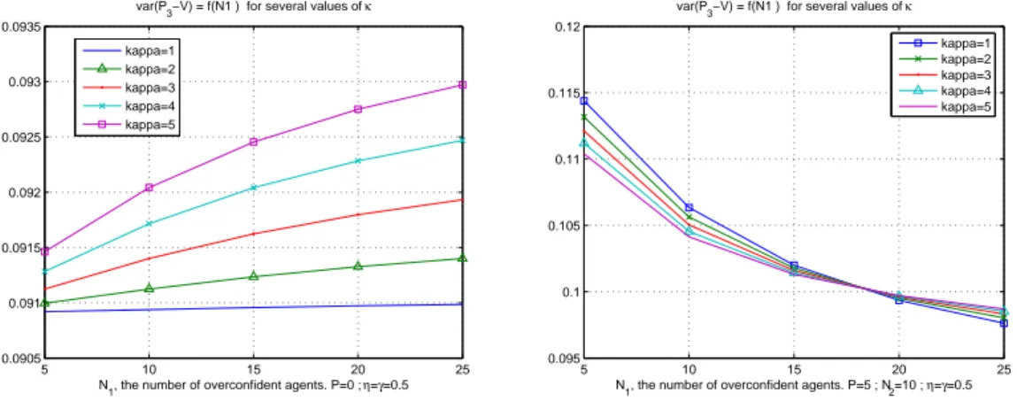
Figure 7, below, shows the ambiguous impact of the number of feedback traders on the quality
of prices. As said before, when P = 0 the quality of prices decreases with both N1 (number
of overconfident traders) and κ (level of overconfidence). When P 6= 0, the quality of prices
increases with N1 and is non-monotonic with κ.
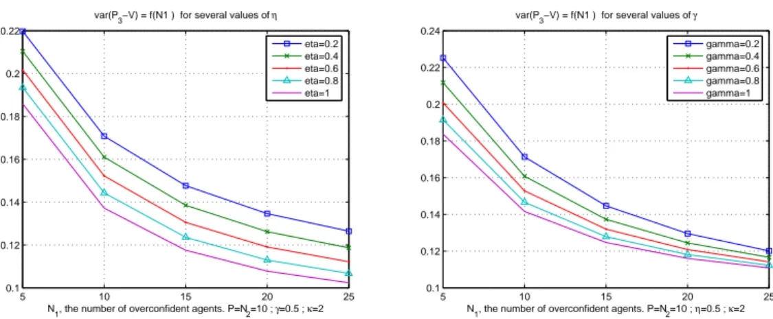
In figure 8, we observe that the quality of prices diminishes when each overconfident trader underestimates the ability of the other ones.
4Ko and Huang (2007) show that arrogance can be a virtue. Indeed, overconfident investors believe that
they can earn extraordinary returns and will consequently invest resources in acquiring information pertaining to financial assets. In our model there is no information-seeking activity which could permit to obtain such a positive externality.
5 10 15 20 25 5 10 15 20 25 0 1 2 3 4
N1, the number of overconfident agents var(P3−V) = f(P ,N1 ). N2=10 ; η=γ=0.5 ; κ=2
P, the number of feedback traders 0.15 10 15 20 25 0.12 0.14 0.16 0.18 0.2 0.22 0.24
N1, the number of overconfident agents. N2=P=10 ; η=γ=0.5 var(P3−V) = f(N1 ) for several values of kappa
kappa=1 kappa=2 kappa=3 kappa=4 kappa=5
Figure 6: The quality of prices at time t = 3 as a function of the number of overconfident traders and
of the parameter κ. 5 10 15 20 25 0.0905 0.091 0.0915 0.092 0.0925 0.093 0.0935
N1, the number of overconfident agents. P=0 ; η=γ=0.5
var(P3−V) = f(N1 ) for several values of κ
kappa=1 kappa=2 kappa=3 kappa=4 kappa=5 5 10 15 20 25 0.095 0.1 0.105 0.11 0.115 0.12
N1, the number of overconfident agents. P=5 ; N2=10 ; η=γ=0.5
var(P3−V) = f(N1 ) for several values of κ
kappa=1 kappa=2 kappa=3 kappa=4 kappa=5
Figure 7: The quality of prices at time t = 3 as a function of the number of overconfident traders and
of the parameter κ, for P = 0 and P = 5.
3.3
Serial Correlation of Prices
Proposition 3.4 The price changes are more important when the number of positive feedback
traders is large.
The serial correlation of prices depends critically on the overconfidence level and on the number of positive feedback traders. In the presence of positive feedback trading, the serial correlation is generally negative. It implies that positive feedback trading destabilizes the price schedule. Informed traders cannot keep price at fundamentals or dampen the fluctuation of prices.
The term cov(P3 − P2, P2 − P1) describes the correction phase in Daniel, Hirshleifer and
Subrahmanyam (1998). They show that overconfident traders begin by overreacting to their private signals. In the second phase, irrational market participants correct their beliefs and
5 10 15 20 25 0.1 0.12 0.14 0.16 0.18 0.2 0.22
N1, the number of overconfident agents. P=N2=10 ; γ=0.5 ; κ=2 var(P3−V) = f(N1 ) for several values of η
eta=0.2 eta=0.4 eta=0.6 eta=0.8 eta=1 5 10 15 20 25 0.1 0.12 0.14 0.16 0.18 0.2 0.22 0.24
N1, the number of overconfident agents. P=N2=10 ; η=0.5 ; κ=2 var(P3−V) = f(N1 ) for several values of γ
gamma=0.2 gamma=0.4 gamma=0.6 gamma=0.8 gamma=1
Figure 8: The quality of prices at time t = 3 as a function of the number of overconfident traders and
of the parameters η and γ.
their order as new public information arrives, this is defined as the “correction phase”. In our model, agents updates their beliefs concerning their private information. The informed market participants know that their earlier trades move prices away from fundamentals as they try to exploit the presence of feedback trading. The size of the departure of prices from fundamentals increases with the number of feedback traders. At date 3, informed participants abruptly correct their demands after observing their last signal. Odean (1998) has found such negative correlation by considering only overconfident agents. We extend his result, as we show that informed rational traders cannot prevent irrational traders (feedback agents as well optimistic traders) to destabilize prices. In our model, the “correction phase” appears as a bubble crash.
In the next two figures we have simulated the price changes as a function of the number of positive feedback traders. Figure 9 shows that the returns reversal increases with the number of feedback traders. This result is reinforced by the level of overconfidence in the market. Figure 10 confirms the previous result, however it shows that the price change is less important when each irrational informed trader underestimates the precision of the other specific market participants’ signals.
3.4
Trading Volume
Proposition 3.5 The trading volume increases with the number of feedback positive traders in
the market.
In the presence of positive feedback trading strategies, informed agents trade more aggressively. They anticipate that the initial price increase will stimulate buying by feedback traders at the subsequent auctions. In doing so, they drive prices up higher than fundamentals. Consequently, feedback positive traders respond by trading even more. We find that the feedback trading as
0 20 40 60 0 10 20 30 −0.03 −0.025 −0.02 −0.015 −0.01 −0.005
N1, the number of ove cov(P3−P2,P2−P1) = f(P ,N1 ). N2=10 ; η=γ=0.5 ; κ=2
P, the number of feedback traders
cov(P 3 −P 2 ,P2 −P 1 ) 5 10 15 20 25 30 −0.045 −0.04 −0.035 −0.03 −0.025 −0.02 −0.015 −0.01 −0.005 0
P, the number of feedback traders. N1=N2=10 ; η=γ=0.5
cov(P 3 −P 2 ,P2 −P 1 )
cov(P3−P2,P2−P1) = f(P ) for several values of kappa kappa=1 kappa=2 kappa=3 kappa=4 kappa=5
Figure 9: The price changes as a function of the number of feedback traders and of the number of
overconfident traders. 5 10 15 20 25 30 −0.07 −0.06 −0.05 −0.04 −0.03 −0.02 −0.01 0 0.01 0.02
P, the number of feedback traders. N1=N2=10 ; γ=0.5 ; κ=2
cov(P 3 −P 2 ,P 2 −P 1 )
cov(P3−P2,P2−P1) = f(P ) for several values of :eta eta=0.2 eta=0.4 eta=0.6 eta=0.8 eta=1 5 10 15 20 25 30 −0.05 −0.045 −0.04 −0.035 −0.03 −0.025 −0.02 −0.015 −0.01 −0.005 0
P, the number of feedback traders. N1=N2=10 ; η=0.5 ; κ=2
cov(P 3 −P 2 ,P 2 −P 1 )
cov(P3−P2,P2−P1) = f(P ) for several values of gamma gamma=0.2 gamma=0.4 gamma=0.6 gamma=0.8 gamma=1
Figure 10: The price changes as a function of the number of feedback traders for different values of η
and γ.
well as the overconfidence enhances the trading volume. Our result is consistent with empirical findings. For instance, Glaser and Weber (2007) (could not find reference) have shown that investors who think that they are above average in terms of investment skills or past performance trade more.
In figure 11, we show that the volume from overconfident traders is a non-monotonic function of κ. For large values of P , this volume decreases with κ.
In figure 12, we show that the volume originating from positive feedback traders increases with the number of feedback agents. It decreases with the level of overconfidence (measured by κ) and it increases with the underestimation the precision of the other overconfident agents’ signal. In figure 13, we compare the volume from overconfident traders and from rational traders with no feedback traders. As expected, we see that overconfident traders trade more aggressively than
5 10 15 20 25 30 0 10 20 30 40 50 60 70 80 90
P, the number of feedback traders. N1=N2=10 ; η=γ=0.5 overconfident trading volume = f(P ) for several values of kappa
kappa=1 kappa=2 kappa=3 kappa=4 kappa=5 5 10 15 20 25 30 0 20 40 60 80 100 120 140 160
P, the number of feedback traders. N1=N2=10. η=γ=0.5 rational trading volume = f(P ) for several values of kappa
kappa=1 kappa=2 kappa=3 kappa=4 kappa=5
Figure 11: The total individual informed orders as a function of the number of feedback traders, for
different values of the parameter κ.
5 10 15 20 25 30 10 20 30 40 50 60 70 80
P, the number of feedback traders. N1=N2=10. η=γ=0.5
feedback trading volume = f(P ) for several values of kappa
kappa=1 kappa=2 kappa=3 kappa=4 kappa=5 5 10 15 20 25 30 0 10 20 30 40 50 60 70 80 90
P, the number of feedback traders. N1=N2=10 ; γ=0.5 ; κ=2
feedback trading volume = f(P ) for several values of eta eta=0.2 eta=0.4 eta=0.6 eta=0.8 eta=1
Figure 12: The total individual feedback trading volume as a function of the number of feedback traders,
for different values of the parameters κ and η.
their rational counterparts. The volume from overconfident investors increases with κ, whereas the volume from rational investor’s order decreases with κ.
4
Profits
We now look at expected profits.
Proposition 4.6 Gains from trade:
• Positive feedback traders always earn negative profits.
• If there are enough positive feedback traders, both overconfident and rational traders can earn positive profits.
5 10 15 20 25 30 3.5 4 4.5 5 5.5 6 6.5 7 7.5 8
N1, the number of overconfident agents. P=0 ; N2=10 ; η=γ=0.5 overconfident trading volume= f(N1 ) for several values of kappa
kappa=1 kappa=2 kappa=3 kappa=4 kappa=5 5 10 15 20 25 30 2.7 2.75 2.8 2.85 2.9 2.95 3 3.05
N1, the number of overconfident agents. P=0 ; N2=10 ; η=γ=0.5 rational trading volume = f(N1 ) for several values of kappa
kappa=1 kappa=2 kappa=3 kappa=4 kappa=5
Figure 13: The total individual overconfident trading volume as a function of the number of overconfident
agents, for different values of the parameter κ.
• When the number of trend chasers is large, overconfident traders earn more than rational speculators. Nevertheless, the profit earned by overconfident decreases with b. When b is large, they realize losses.
Positive feedback traders act as pure noise traders since they are uninformed. Such trading behavior leads these agents to always lose money. Informed agents anticipate their strategy. In doing so, they introduce at the earlier auctions noise which is enhanced by the positive feedback traders themselves at the last rounds.
When there are only rational and overconfident traders in the market, we find that overconfident traders earn less profit than their rational counterparts. This result is consistent with, among others, Odean (1998), and Gervais and Odean (2001). When the 3 types of traders are present (overconfident, rational and positive feedback agents) overconfident agent may outperform ra-tional traders. This result confirms Benos (1998) and Germain et al. (2009). Indeed in Benos (1998) and Germain et al. (2009), pure noise traders trading for liquidity reasons are present. However, in our model, overconfident traders earn more profits than their rational counterparts as they trade less aggressively. They believe that the main reason for prices to be different from fundamentals is the presence of trend-chasers. Moreover, Benos (1998) analyzes a static market and overconfident market participants cannot correct their earlier trades in the last auctions. We now look at the different simulations we have performed regarding the expected profits for the different traders present in the market.
Firstly, we obtain, as anticipated, that positive feedback traders always realize losses, their losses increase with the number of positive feedback traders (see figure 14).
We look now at the influence of the different overconfidence parameters on the positive feedback trader’s profit.
The figure below (figure 15) shows that positive feedback trader’s losses are less important when each overconfident trader treats his own private information as being better than it is, as captured by the parameter κ. It also shows that the higher the overconfidence parameters η and γ, the more severe the positive feedback traders’ losses are. These results stem from the fact that the trend-chasers’ trading volume decreases with κ and increases with η and γ.
5 10 15 20 25 5 10 15 20 25 −400 −300 −200 −100 0
N1, the number of overconfident agents
Total individual feedback trader’s profit f = f(P ,N1 ). η=γ=0.5 ; κ=2
P, the number of feedback traders
5 10 15 20 25 −160 −140 −120 −100 −80 −60 −40 −20 0
P, the number of feedback traders. N1=N2=10 ; η=γ=0.5
total individual feddback trader’s profit f = f(P ) for several values of kappa kappa=1 kappa=2 kappa=3 kappa=4 kappa=5
Figure 14: The total individual positive feedback trader’s profit as a function of the number of
over-confident agents and of the number of positive feedback traders, for different values of the parameter κ. 5 10 15 20 25 −250 −200 −150 −100 −50 0
P, the number of feedback traders. N1=N2=10 ; γ=0.5 ; κ=2
Total individual feedback trader’s profit f = f(P ) for several values of eta eta=0.2 eta=0.4 eta=0.6 eta=0.8 eta=1 5 10 15 20 25 −300 −250 −200 −150 −100 −50 0
P, the number of feedback traders. N1=N2=10 ; η=0.5 ; κ=2
Total individual feedback trader’s profit f = f(P ) for several values of gamma gamma=0.2 gamma=0.4 gamma=0.6 gamma=0.8 gamma=1
Figure 15: The total individual positive feedback trader’s profit as a function of the number of positive
feedback traders, for different values of the parameters η, γ.
In figure 16, we can observe that the individual expected profits of overconfident traders decrease with b. Nevertheless, when the mean bias is not too high, overconfident agents earn positive expected profit when there are enough positive feedback traders. Similarly to Germain et al. (2009), we find that the mean bias affects the investors’ trading volumes and therefore their profits. Indeed, when the mean bias b increases, overconfident agents trade more aggressively in the wrong direction, as a result they incur large losses. These losses may be reduced if a large number of positive feedback traders are present in the market. Finally, in figure 16, we observe
that for an overconfident trader a misinterpretation about the precision of the fundamental value
(hv) is worse than an error of judgment on his specific own private information (hε).
5 10 15 20 25 −150 −100 −50 0 50 100
P, the number of positive feedback traders. N1=N2=10 ; η=γ=0.5 ; κ=2 Total individual overconfident trader’s profit b = f(P ) for several values of b
b=0 b=2 b=4 b=6 b=8 b=10 0.2 0.4 0.6 0.8 1 1 2 3 4 5 −40 −20 0 20 40 60 eta
Total individual overconfident trader’s profit b = f(kappa ,eta ). N1=N2=P=10 ; γ=0.5 ; b=2
kappa
Figure 16: The total individual overconfident trader’s profit as a function of the number of positive
feedback traders, for different values of the mean bias b of the overconfidence. And the total individual overconfident trader’s profit as a function of the parameters κ and η.
5
Discussion
In this part, we are interested in understanding how price bubbles may arise in a financial market. We have shown that positive feedback trading induces an price volatility and worsens market efficiency more than overconfident trading. When positive feedback agents are introduced into the market, overconfident investors may make more profit than rational speculators. However, positive feedback traders can suffer very important losses if they are too many in the market. On the other hand, a financial bubble can be characterized by an important gap between market price and fundamentals. Since overconfident agents receive private signals about fundamentals, they trade on private information and exploit the presence of feedback traders. Only, feed-back trading can trigger a bubble. As a result overconfident traders may worsen the bubble
phenomenon as well as the collapse of the bubble.5
To see the bubble phenomenon, we have simulated prices over the time according to the number of positive feedback traders, the number of overconfident traders and the mean bias of the overconfident agents. Moreover, we also focus on the effect of the risk aversion coefficient a. Figure 17 confirms that the bubble phenomenon depends mainly on the number of feedback traders. Feedback trading is based on the previous prices movement and it may appears as a lagged trading. Abreu and Brunnermeier (2003) have shown that the synchronization problem can be a reason for the persistence of bubbles. In their model, rational arbitrageurs face a lack of synchronization because there are different optimal timing trading strategies. The bubble can grow and last as long as there is a sufficient number of rational traders to sell out. In our model, when the mass of informed traders is very large in comparison with the feedback trading, bubbles cannot exist.
In figure 18, we observe that the volatility of price and the price change increase with the risk aversion coefficient. Informed investors react abruptly to new information and provoke prices to be more volatile. This result emphasizes that the risk aversion of the market participants can explain part of the excess volatility observed in the market.
Figure 19 shows that the price changes is less extreme when the market participants are less risk averse. Moreover, the difference between the overconfident investors ’demand and the rational one is more depend on the strength of the positive feedback trading than the risk aversion of the speculators.
The presence of bubbles and crashes is mainly explained by two factors: the positive feedback trading and the risk aversion of the investors. The overconfidence has an important impact on the volatility of prices, on the trading volume and on the wealth of the informed traders without
5
Feedback trading is often cited as the reason of the bubble (see Zhou and Sornette (2006, 2009), Cajuueiro, Tabak and Werneck (2009), and Johansen, Ledoit, and Sornette (2003).
0 1 2 33 10 12 14 16 18 20 22 24 26 28 t. N1=N2=10 ; η=γ=0.5 ; κ=2 Price = f(t ) for several values of P P=5 P=10 P=15 P=20 P=25 0 0.5 1 1.5 2 2.5 3 10 12 14 16 18 20 22 t. N2=P=10 ; η=γ=0.5 ; κ=2 Price = f(t ) for several values of N1 N1=5
N1=10 N1=15 N1=20 N1=25
Figure 17: Prices over time for different values of P (the number of positive feedback traders) and for
different values of N1 (the number of overconfident agents).
5 10 15 20 25 0.5 1 1.5 2 2.5 3 3.5 4
P, the number of feedback traders. N1=N2=25 ; η=γ=0.5 ; κ=2
var(P3) = f(P ) for several values of a
a=1 a=2 a=3 a=4 a=5 5 10 15 20 25 −0.022 −0.02 −0.018 −0.016 −0.014 −0.012 −0.01
P, the number of feedback traders. N1=N2=25 ; η=γ=0.5 ; κ=2
cov(P3−P2,P2−P1) = f(P ) for several values of a
a=1 a=2 a=3 a=4 a=5
Figure 18: The volatility of prices at date t = 3 and the cov(P3− P2, P2− P1), for different values of the
parameter a.
provoking the growth and the burst of bubbles. Nevertheless, in the presence of feedback trading, risk averse overconfident investors can enhance the volatility of prices and both the bubble and crash phenomenon too.
For the sake of exposition we dedicate the next section to contrarian trading, i.e. feedback traders selling (buying) when prices increase (decrease).
6
On Contrarian Trading
In this section we look at the case of contrarian trading.
First of all, it should be noticed that due to their trading behaviour, the negative feedback traders limit the movement of prices. Informed traders upon receiving some information will
0 1 2 3 10 12 14 16 18 20 22 24 t. N1=N2=25 ; P=15 ; η=γ=0.5 ; κ=2 Price = f(t ) for several values of a a=1 a=2 a=3 a=4 a=5 5 10 15 20 25 1 2 3 4 5 −10 −5 0 5 P
Difference between overconfident and rational trading volume = f(a ,P )
a
Figure 19: Price over time for different values of a and difference of demands between overconfident and
rational investors.
always follow their information and trade larger quantities as they know that due to negative feedback trading subsequent prices will not fully reflect their information (I think! This should be checked with simulations). This alters some of the comparative statics we found earlier for the case of positive feedback trading. The reader can refer to the figures in the Appendix, at the end of the paper, for the different comparative statics.
We find the obvious result that the volatility of prices decreases with the number of negative feedback. This volatility of prices increases with the number of overconfident.
The quality of prices in both periods decreases with the number of negative feedback whereas the quality of prices in the third period increases with the number of overconfident and with κ.
The serial correlation is negative and decreases with the number of negative feedback. The overall volume traded by rational investors increases with the number of negative feed-back and decreases with the level of overconfidence in the market, κ. An interesting result arises, when we look at the overall volume traded by overconfident traders. For a low number of feed-back traders, the volume traded by overconfident decreases with P whereas for a large number of feedback traders it increases with P . The range for which it decreases with P increases as the level of overconfidence, κ, increases.
Finally, we find that the expected profit of the negative feedback traders decreases with the number of negative feedback present in the market and that they can derive positive expected profits for a low number of negative feedback traders. In that case the second round gains com-pensate the third round losses. However, as overconfident traders become more overconfident, measured by an increase of κ, the expected profit decreases.
Conclusion
In this paper, we have analyzed the effects of overconfidence and trend-chasing behavior on financial markets.
According to our model, when there are only overconfident agents in the market, no sig-nificant bubbles arise. However, overconfidence noticeably affects trading volume and profit. Overconfident agents tend to trade very aggressively as they overreact to information. Overre-action to information is the main reason why overconfident agents increase volatility and decrease the quality of prices.
When overconfident agents are competing with rational traders, they tend to have the same behavior as described previously. They trade very aggressively and tend to increase the price volatility and to decrease the quality of the prices in the market. The higher the proportion of overconfident traders, the more these agents trade and as a reaction the less rational participants trade. Rational traders always earn larger expected profit than overconfident traders. In such a market, bubbles do not appear.
Eventually, when overconfident, rational and feedback positive traders participate in the market, the situation tends to be a little different from the two previous ones. Positive feedback
traders increase price volatility. Their trade is based on past prices which are determined
by the informed trading in earlier stages. This causes a temporary miscoordination between traders. This phenomenon is amplified by the fact that both overconfident and rational traders anticipate the behavior of feedback-positive agents. As a result feedback traders never generate profits. When there are few feedback traders in the market, both overconfident and rational traders are unable to earn positive expected profit. When feedback traders are very numerous, both overconfident and rational investors earn positive expected profit. In both situations, overconfident traders are always better off than rational traders.
7
References
Abreu, D., and Brunnermeier, M.K, (2003). Bubbles and Crashes. Econometrica, 71 (1) pp. 173-204.
Andreassen, P., Kraus, S., (1990). Judgmental Extrapolation and the Salience of Change. Journal of Forecasting, 9 pp. 347-372.
Barber, B.M., Odean, T., (2001). Boys Will be Boys: Gender, Overconfidence, and Common Stock Investment. Quarterly Journal of Economics, Vol. 116 (1) pp. 261-292.
Benos, A. V., (1998). Aggressiveness and Survival of Overconfident Traders. Journal of Fi-nancial Markets 1 pp. 353-383.
Bernoulli, Daniel, (1954). Exposition of a New Theory.
Biais, B., Hilton, D., Mazurier, K., Pouget, S., (2005). Judgemental Overconfidence, Self-Monitoring and Trading Performance in an Experimental Financial Market. Review of Economic Studies, Vol. 72(2).
Bohl, M.T., Brzeszczynski, J., (2006). Do Institutional Investors Destabilize Stock Prices? Evidence from an Emerging Market. International Financial Markets, Institutions and Money 16, pp. 370-383.
Bohl, M.T., Siklos, P.L., (2005). Trading Behavior During Stock Market Downturns: The Dow, 1915 — 2004. Working Paper.
Caballé, J., Sákovics, J., (2003). Speculating Against an Overconfident Market. Journal of Financial Markets Vol. 6, pp. 199-225.
Campbell, J.Y., Kyle, A.S.,(1988). Smart Money, Noise Trading and Stock Price Behavior. Review of Economic Studies 60(1), pp. 1-34.
Chau, F., Holmes, P., Paudyal, K. (2005). The Impact of Universal Stock Futures on Feedback Trading and Volatility. Journal of Business Finance and Accounting Vol. 35(1-2), pp. 227-249.
Daniel, K., Hirshleifer, D., Subrahmanyam, A., (1998). Investor Psychology and Security Market Under- and Overreactions. Journal of Finance 53(6), pp. 1839-1885.
DeBondt, W.F.M., Thaler, R.H., (1985). Does The Stock Market Overreact? Journal of Finance 40, pp. 793-808.
DeBondt, W.F.M., Thaler, R.H., (1987). Further Evidence on Investor Overreaction and Stock Market Seasonality. Journal of Finance 42, pp. 557-581.
De Bondt, W.F.M, Thaler, R.H., (1990). Do Security Analysts Overreact? American Economic Review 80(2), pp. 52-57.
De Long, J.B., Shleifer, A., Summers, L.H., and Waldmann R.J. (1990). Positive Feedback Investment Strategies and Destabilizing Rational Speculation. Journal of Finance 45. Dennis, P., and Deon Strickland, D., (2002). Who Blinks in Volatile Markets, Individuals or
Institutions? Journal of Finance 57(5), pp. 1923-1949.
Dow, J., Gorton, G., (1997). Noise Trading, Delegated Portfolio Management, and Economic Welfare. Journal of Political Economy 105(5), pp. 1024-1050.
Evans, M., Lyons, R., (2003). How is macro news transmitted to exchange rates? Journal of Financial Economics 88, pp. 26-50.
Fama, E.F., (1965). The Behavior of Stock Market Prices. Journal of Business, pp. 34-105. Fama, E.F., (1970). Efficient Capital Markets : A Review of Theory and Empirical Work.
Journal of Finance 25, pp. 383-417.
Figlewski, S., (1979). Subjective Information and Market Efficiency In a Betting Market. Journal of Political Economy 87, pp. 75-88.
Frankel, J, Froot, K., (1988). Explaining The Demand For Dollars: International Rates of Return and The Expectations of Chartists and Fundamentalists. R. Chambersand P. Paarlberg eds., Agriculture, Macroeconomics, and The Exchange Rate (Westfield Press, Boulder, Co).
Germain, L., Rousseau, F., Vanhems, A., (2009). Irrational Financial Markets, Working Paper. Gervais, S., Odean, T., (2001). Learning to be Confident. Review of Financial Studies 14 (1),
pp. 1-27.
Glaser, M., Nöth, M., and Weber, M., (2004), Behavioral Finance, in Blackwell Handbook of Judgment and Decision Making, ed. by D. J. Koehler, and N. Harvey. Blackwell, Malden, Mass., pp. 527-546.
Grether, D., (1980). Bayes’ rule as a Descriptive Model: The representative Heuristic. Quar-terly Journal of Economics 95, pp. 537-557.
Hirshleifer, D., Subrahmanyam, A., Titman, S., (2006). Feedback and the success of irrational investors. Journal of Financial Economics 81, pp. 311-338.
Kahneman, D., Tversky, A., (1973). On the Psychology of Prediction. Psychological Review 80, pp. 237-251.
Kaizoji, T., (2000). Speculative bubbles and crashes in stock markets: an interacting-agent model of speculative activity. Physica A 287, pp. 493-506.
Kunieda, T., (2007). Asset Bubbles and borrowing constraints. Journal of Mathematical Economics 44, pp. 112-131.
Kyle, A. S. (1985). Continuous Auctions and Insider Trading. Econometrica 53(6), pp. 1315-1336.
Kyle, A. S., Wang., F. A., (1997). Speculation Duopoly with Agreement to Disagree: Can Overconfidence Survive the Market Test. Journal of Finance 52(5), pp. 2073-2090. Lakonishok,J., Shleifer, A., Vishny, R.W., (1994). Contrarian Investment, Extrapolation, and
Risk. Journal of Finance 49(5), pp. 1541-1578.
Mardyla, G., Wada, R., (2009, forthcoming). Individual Investors’ Trading Strategies and Re-sponsiveness to Information - A virtual Stock Market Experiment. Ritsumeikan University. Keiai University.
Odean, T., (1998). Volume, Volatility, Price, and Profit When All Traders Are Above Average. Journal of Finance 53(6), pp. 1887-1934.
Shu, T., (2009). Does Positive-Feedback Trading by Institutions Contribute to Stock Return Momentum? Working Paper University of Georgia.
Sias, R.W., Starks, L.T., (1997). Return autocorrelation and institutional investors. Journal of Financial Economics 46(1), pp. 103-131.
Sias, R.W., Starks, L.T., Titman, S., (2001). The Price Impact of Institutional Trading. Washington State University and University of Texas at Austin.
Sornette, D.,and Zhou, W.X., (2006). Is There a Real Estate Bubble in the US ? Physica A. 361, pp. 297-308.
Sornette, D.,and Zhou, W.X., (2009). A Case Study of Speculative Bubble in the South African Stock Market 2003-2006. School of Business, East China University of Science and Technology, Shanghai 200237, China
Soros, G., (1987). The Alchemy of Finance. Simon and Schuster, New York.
Statman, M., Thorley, S., Vorkink, K., (2006). Investor Overconfidence and Trading Volume. Review of Financial Studies 19(4), pp. 1531-1565.
Appendix
Proof of Proposition 2.1: Equilibrium
This proposition is proved by backward induction, we then start with the last period, i.e. t = 3.
7.0.1 Third round t = 3
At time t = 3, each trader, noted i, has private information Φ3i which has a multivariate
distribution. The information available for trader i is : Φ3i= [y2i, y3i, P2, P3]T.
An overconfident trader infers the mean of this distribution, Eb(Φ3i), and the
variance-covariance matrix, Ψb, as follows:
Eb(Φ3i) = [¯v + b, ¯v + b, α21+ α22(¯v + b), α31+ (α32+ α33)(¯v + b)]T, Ψb= ⎡ ⎢ ⎢ ⎢ ⎣ 1 ηhv + 1 κhε 1 ηhv α22 ηhv + α22 M κhε α32+α33 ηhv + α32 M κhε 1 ηhv 1 ηhv + 1 κhε α22 ηhv α32+α33 ηhv + α33 M κhε α22 ηhv + α22 M κhε α22 ηhv α2 22 ηhv + α2 22(γ+M κ−κ) M2κγh ε C1 α32+α33 ηhv + α32 M κhε α32+α33 ηhv + α33 M κhε C1 C2 ⎤ ⎥ ⎥ ⎥ ⎦, with C1 = α22ηhαv33 + α22α32 ³ 1 ηhv + γ+Mκ−κ M2κκγh ε ´ , and C2 = (α32+α33) 2 ηhv + (α32+ α33) 2³γ+M κ−κ M2κγh ε ´ .
The mean, Er(Φ3i), and the variance-covariance matrix Ψrfor the rational agent are obtained
by setting b = 0, η = κ = γ = 1 in Eb(Φ3i) and Ψb.
By solving the mean-variance problem, we obtain the ith insider’s orders: xb3i= Eb(˜v|Φ3i) − P3 avarb(˜v|Φ3i) , xr3i= Er(˜v|Φ3i) − P3 avarr(˜v|Φ3i) .
On the other hand, we know that each feedback trader i determines her order by considering the trend of prices as follows :
xf3i= β(P2− P1). Using the projection theorem, we obtain the following
Eb(˜v| ˜Φ3i) = (y2i+ y3i)(κ − γ)hε+ ( ¯Y2+ ¯Y3)γhεM + ηhv(¯v + b) ηhv+ 2(κ + γM − γ)hε, varb(˜v|Φ3i) = 1 ηhv+ 2(κ + γM − γ)hε , Er(˜v|Φ3i) = ( ¯Y2+ ¯Y3)hεM + hvv¯ hv+ 2M hε , varr(˜v|Φ3i) = 1 hv+ 2M hε .
Replacing the above into the expressions of the different orders for the different types of traders we obtain
xb
3i = 1a[(y2i+ y3i)(κ − γ)hε+ ( ¯Y2+ ¯Y3)γhεM + ηhv(¯v + b) − P3(ηhv+ 2(κ + γM − γ)hε)],
xr3i = 1a[( ¯Y2+ ¯Y3)hεM + hvv − P¯ 3(hv+ 2M hε)],
xf3i = β(P2− P1).
In equilibrium the total demand must be equal to the exogenous total supply, this is given by N1 X i=1 xb3i+ N2 X i=1 xr3i+ P X i=1 xf3i= (N1+ N2+ P )¯x. (7.3)
From (7.3), the price P3 can be obtained as a function of ¯Y2, ¯Y3, P2 and P1
P3=
1
Λ[((N1γ + N2)M hε+ (κ − γ)N1hε) ( ¯Y2+ ¯Y3) + (N1η + N2)hvv + N¯ 1ηhvb
− a(N1+ N2+ P )¯x + aP β(P2− P1)],
with Λ = (N1η + N2)hv+ 2(N1(κ + γM − γ) + N2M )hε, ¯Y2 = ˜v + εM2i +M1Pj6=iε2j and ¯Y3 =
˜ v + ε3i M + 1 M P j6=iε3j.
α31 = (N1η+N2)hvv+N¯ 1ηhΛvb−a(N1+N2+P )¯x +aP βΛ (α21− P1),
α32 = N1(κ+γM −γ)hΛ ε+N2M hε +aβPΛ α22,
α33 = N1(κ+γM −γ)hΛ ε+N2M hε.
7.0.2 Second round t = 2
Using the third round’s results, we can obtain the second round’s parameters.
Let us introduce the following notations where b stands for the overconfident trader whereas r stands for the rational one:
BbT = covb(P3, Φ2i) = [covb(y2i, P3), covb(P2, P3)],
BrT = covr(P3, Φ2i) = [covr(y2i, P3), covr(P2, P3)]. Using the projection theorem, we get
Ej(P3|Φ2i) = Ej(P3) + BjTvarj(Φ2i)−1(Φ2i− Ej(Φ2i)), varj(Φ2i) = µ varj(y2i) α22covj(y2i, ¯Y2) α22covj(y2i, ¯Y2) α222varj( ¯Y2) ¶ ,
where j = b, r and Ej and varj denote the fact that they are computed following trader j’s
beliefs. We obtain Ej(P3|Φ2i) = (α32+ α33)¯vj + α31+L1j((covj(y2i, P3)Dj1+ covj(P2, P3) Dj3 α22)(y2i− ¯v) +covj(y2i, P3)Dj3+ covj(P2, P3) Dj2 α22( ¯Y2− ¯v)),
varj(P3|Φ2i) = varj(P3) − L1j(Dj1covj(y2i, P3)2+ 2D3j α22covj(y2i, P3)covj(P2, P3) +D j 2 α2 22 covj(P2, P3)2), with ¯ vj = ½ ¯ v if j = r ¯ v + b if j = b , Db1= varb( ¯Y2) = ηh1v + (γ+Mκ−κ)M2γκh ε , Db 2= varb(y2i) = ηh1v +κh1ε, Db3= −covb(y2i, ¯Y2) = − ³ 1 ηhv + 1 M κhε ´ ,
Lb = varb(y2i)varb( ¯Y2) − covb(y2i, ¯Y2)2 = (M−1)[((M−1)γ+κ)hM2ηκγh ε+ηhv] vh2ε ,
D1r, D1r, Dr3, and Lr can be obtained by setting κ = γ = η = 1 in Db1, D1b, Db3, and Lb. At the second round, informed trader i’s order is:
xb2i= Eb(P3|Φ2i) − P2 avarb(P3|Φ2i) , xr2i= Er(P3|Φ2i) − P2 avarr(P3|Φ2i) .
The ith feedback agent’s order is:
xf2i= β(P1− P0). By equalizing exogenous supply and demand, we have:
(N1+ N2+ P )¯x = N1 X i=1 Eb(P3|Φ2i) − P2 avarb(P3|Φ2i) + N2 X i=1 Er(P3|Φ2i) − P2 avarr(P3|Φ2i) + P β(P1− P0). 7.0.3 First round t = 1
At the first round, none of the traders participating to the market are informed. The different agents’ orders are:
xr1i= Er(P2) − P1 avarr(P2) = α21+ α22v − P¯ 1 aα2 22varr( ¯Y2) , xb1i= Eb(P2) − P1 avarb(P2) = α21+ α22(¯v + b) − P1 aα2 22varb( ¯Y2) ,
There are no feedback traders in the first round. However, the agents who will become informed subsequently anticipate the presence of such behavior for the next two rounds.
Again, the no-excess supply equation leads to
(N1+ N2)¯x = N1 X i=1 xb1i+ N2 X i=1 xr1i.
The price P1 can then be derived:
P1= α21+ α22¯v +−aα
2
22x(N¯ 1+ N2)varr( ¯Y2)varb( ¯Y2) + N1α22bvarr( ¯Y2) N1varr( ¯Y2) + N2varb( ¯Y2)
From the above expression the parameters α21 and α22 can be identified.
After some computations, one can show that α22 = caβP +dN where N is independent of P ,
with c = −[Z1(zhε+ ηhv) + Z2(M hε+ hv)], d = ΛηhvM2κγhε2LbLr(N1varr(P3|Φ2i) + N2varb(P3|Φ2i)), N = Z1Z3hε(ηhv+ 2hεj) + Z2Z3hε(hv+ 2M hε), Z1 = N1varr(P3|Φ2i)Lr(M − 1), Z2 = N2varb(P3|Φ2i)Lb(M − 1)ηκγ, Z3 = N1z + N2M, z = κ + γM − γ, varb(P3|Φ2i) = α233hη (κ (M − 1) + γ) hv+ ³ (M − 1) (κ − γ)2+ 2M κγ´hε i M2γκh ε(zhε+ ηhv) , Lb = M2γ + M (κ + η − 2γ) + γ − κ − η ηγκM2h vhε ,
where varr(P3|Φ2i) and Lr can be obtained by setting γ = κ = η = 1 in the expressions of
varb(P3|Φ2i) and Lb.
It can be shown after some tedious computations that c < 0, d > 0 and N > 0.
Once α22 has been determined, the other parameters can be derived.
Proof of Proposition 3.2
We now derive the variance of prices with respect to P .
t= 2
The variance is given by var(P2) = α222var( ¯Y2) with α22 = caβP +dN . After some tedious
computations it can be shown that c < 0, d > 0 and N > 0.
The derivative of var(P2) with respect to P is then equal to
∂var(P2) ∂P = ∂α222 ∂P var( ¯Y2) = 2α22 ∂α22 ∂P var( ¯Y2) = 2α22 µ −c(cP + d)N 2 ¶ var( ¯Y2).
Given that var( ¯Y2) > 0 , α22> 0 and −c(cP +d)N 2 > 0 since c < 0 and N > 0, it can be established
that ∂var(P2)
t= 3
The variance for t = 3 prices is given by
var(P3) = α232var( ¯Y2) + α233var( ¯Y3) + 2α32α33cov
¡¯ Y2, ¯Y3 ¢ , = (α232+ α233)( 1 hv + 1 M hε ) +2α32α33 hv .
Using the fact that α32= α33+aβPΛ α22, we can rewrite the variance of prices as follows
var(P3) = (α33+ aP β Λ α22)[(α33+ aP β Λ α22)( 1 hv + 1 M hε ) +2α33 hv ] + α233( 1 hv + 1 M hε ).
The derivative is then given by the following expression
∂var(P3) ∂P = 2aP βα22 Λ ( α33 hv + (α33+ aP βα22 Λ )( 1 hv + 1 M hε )) > 0.
Proof of Proposition 3.3
We now look at the quality of prices. We first start with t = 2 and then turn to t = 3.
The quality of prices for t = 2 is given by var(P2 − ˜v) which is given by the following
expression var(P2− ˜v) = α222 hv + α 2 22 M hε + 1 hv − 2 α22 hv = (α22− 1) 2 hv + α 2 22. M hε
The derivative with respect to P is positive and given by
∂var(P2− ˜v) ∂P = 2(α22− 1) hv ∂α22 ∂P + 2α22 M hε ∂α22 ∂P = 2 ∂α22 ∂P [ α22− 1 hv + α22 M hε ] >????????0.
For the quality of prices for t = 3, we proceed as for t = 2. The quality of prices is equal to
var(P3− ˜v) = (α32+ α33− 1)2 hv +α 2 32+ α233 M hε .
The derivative is then
∂var(P3− ˜v) ∂P = ∂α32 ∂P µ 2(α32+ α33− 1) hv + 2α32 M hε ¶ >????? 0.
Proof of Proposition 3.4
We have
cov(P3− P2, P2− P1) = cov(P3− P2, P2),
= cov(P3, P2) − cov(P2, P2).
After some manipulations, it can be rewritten as
cov(P3− P2, P2− P1) = α22 ¡ var( ¯Y2) (α32− α22) + α32cov ¡¯ Y2, ¯Y3 ¢¢ .
Using the fact that α32= α33+ aβPΛ α22, cov
¡¯
Y2, ¯Y3 ¢
= h1
v and that var( ¯Y2) =
1 hv+M hε, we obtain cov(P3− P2, P2− P1) = α22 ∙µ α33+ α22 µ aβP Λ − 1 ¶¶ 1 hv+ M hε +α33 hv ¸ .
The derivative with respect to P is then given by
∂cov(P3− P2, P2− P1) ∂P = ∂α22 ∂P α33 µ 2 hv + 1 M hε ¶ + µ aβP Λ − 1 ¶ µ α32 ∂α22 ∂P + α22 ¶ 1 hv+ M hε .
Proof of Proposition 4.6
We now compute the expected profits for all type of traders for each trading round.
Third round profits
The optimistic traders’ expected profit, Πb3i, is given by
Πb3i= E(xb3i(˜v − P3)) = E(xb3iv) − E(x˜ b3iP3),
where the demand, xb3i, is
xb3i= α∗(y2i+ y3i) + β∗(Y2+ Y3) − γ∗P3+ δ∗, with α∗ = (κ−γ)hε a , β∗ = γM hε a , γ∗ = ηhv+2(κ+γ(M −1))hε a and δ∗ = ηhv(v+b) a .
After having computed the two elements of the expected profit and after some simplifications we obtain
Πb3i= (α∗+ β∗)[ 2 hv + 2¯v2− 2α31v − (α¯ 32+ α33)( 2 hv + 2¯v2+ 1 M hε )] (7.4) − γ∗[α31(1 − 2(α32+ α33))¯v − α231+ (α32+ α33)(1 − (α32+ α33))( 1 hv + ¯v2) −(α 2 32+ α233) M hε − α 2 31] + δ∗[¯v(1 − (α32+ α33)) − α31].
We now focus on the rational traders’ expected profit, Πr
3i. In order to compute Πr3i the
same steps as for calculating the expected profit of the optimistic traders can be followed. The
demand for the rational trader, xr
3i, admits the same linear form as the demand for the optimistic
trader. The coefficients are given by α∗= 0, β∗= M hε
a , γ∗ =
hv+2M hε
a and δ∗ =
hv¯v
a .
The rational traders’ expected profit, Πr3i, can be obtained from (7.4) by replacing κ = γ =
η = 1 and b = 0.
The feedback traders’ expected profit Πf3i depends on the first and second round prices P1
and P2 through their demand xf3i= β(P2− P1). It can be computed by computing the following
expression
Πf3i= E(xf3i(˜v − P3)) = E(xf3iv) − E(x˜ f 3iP3). After some computations and simplifications, it is given
Πf3i = β [(α21− P1) (α31+ (1 − (α32+ α33)) ¯v) − α22α31v]¯ + βh(h1 v + ¯v 2)[α 22(1 − α32− α33)] − α22α32M h1ε i .
Second round profit
Similarly to the third round, we have already calculated the price at the second round P2 and
the terms α21 et α22. We can now determine the optimistic traders’ expected profit Πb2i. As
before the expected profit is given by
Πb2i= E(xb2i(˜v − P2)) = E(xb2iv) − E(x˜ b2iP2), where xb2i= Eb[P3/Φ2i]−P2
avarb[P3/Φ2i].
After some computations, we obtain
Πb2i= avar 1 b[P3/Φ2i][(Ab− α21) (−α21+ (1 − α22)¯v) (Sb+ Tb− α22)( 1 hv + ¯v2− α21¯v − α22( 1 hv + ¯v2+ 1 M hε ))],