Damage Detection in Civil Engineering Structure Considering Temperature Effect
Nguyen V.H.
a, Mahowald J.
a, Golinval J.-C.
b, Maas S.
a,
a
University of Luxembourg,
Faculty of Science, Technology and Communication,
Rue Coudenhove – Kalergi, 6; L – 1359 Luxembourg
b
University of Liege,
Department of Aerospace and Mechanical Engineering
1, Chemin des Chevreuils, B 52; B - 4000 Liège 1, Belgium
ABSTRACT: This paper concerns damage identification of a bridge located in Luxembourg. Vibration responses were captured from measurable and adjustable harmonic swept sine excitation and hammer impact. Different analysis methods were applied to the data measured from the structure showing interesting results. However, some difficulties arise, especially due to environmental influences (temperature and soil-behaviour variations) which overlay the structural changes caused by damage. These environmental effects are investigated in detail in this work. First, the modal parameters are identified from the response data. In the next step, they are statistically collected and processed through Principal Component Analysis (PCA) and Kernel PCA. Damage indexes are based on outlier analysis.
Keywords: temperature effect, damage, identification, detection, statistics 1. Introduction
As for mechanical systems, the condition of civil engineering structures such as bridges may be monitored through vibration features identified regularly during their life. Damage detection is often performed by comparison of modal characteristics between current states and an earlier healthy state considered as “reference”. However, detection based on the comparison of modal parameters like natural frequencies, mode shapes etc. is not always obvious, because damage is not the only source that disturbs those parameters. Indeed, environmental factors, i.e. temperature, temperature gradients, traffic etc., show an important influence on modal parameters as well. It was shown through a bridge’s monitoring in HongKong [1] that the normal environmental changes can bring variance error from 0.2% to 1.52% for the first ten eigenfrequencies. Such a high variation may mask the frequency change due to structural damage, which begs the question: how to remove the environmental effects in the damage detection problem.
In face of the last intricate question, several investigations have been carried out on civil engineering structures. Data reduction is often performed from time sequences into modal features. In [2, 3], damage detection was achieved by some derivatives of Principal Component Analysis and factor analysis where numerical data were collected according to a quite large range of temperature. Furthermore experiments in laboratory [4, 5] and on real structures have been examined. In the last decade, the real bridge Z24 in Switzerland was studied in several works [2, 6, 7] with various methods. Damage detection and localization in the I-40 bridge in New Mexico (USA) was also studied in [5, 8]; however, temperature effect was modeled numerically in [5].
The example considered in this paper is the Champangshiel bridge located in Luxembourg. Before it was demolished in 2011, artificial damages were introduced gradually and the bridge was monitored for a short period. Damage detection performed on this bridge is addressed in former works [9, 10, 14]. Damages were well detected, but close examination of eigenfrequency shifts and damage indexes did not allow to clearly identify the levels of damages. It was suspected that it could be due to the variation of ambient conditions. In this context, the present work seeks to remove the temperature effect
in the bridge diagnosis. It consists in Principal Component Analysis (PCA) and its derivative Kernel PCA. The idea is to perform PCA on the identified vibration features in order to separate changes due to environmental variations from changes due to damages. The indication of damage is then based on the prediction error of the model.
2. Detection strategy
Regarding to damage detection, many authors consider eigenfrequencies as good features, although they may be very sensitive to temperature variation. Mode-shapes are less influenced by temperature. In [3], it was shown through a numerical example that damage detection including temperature effect is better when high shapes (modes 6-10) rather mode-shapes at low frequency are considered as features. However, in real-time monitoring of bridges, modes at high frequency can only be identified with more difficulty from vibration measurements. Therefore the features considered in this paper are eigenfrequencies of the bridge. In a first step, eigenfrequencies are identified by applying the Wavelet transform on the recorded signals. Next, they are analyzed using PCA/KPCA in order to differentiate the temperature effect from the damage effect in the feature variations.
2.1. Principal Component Analysis Approach
As described in [2], the technique does not require any measurement of environmental parameters because they are considered as embedded variables. Their effect can be simply observed from the variation of the identified features. The present study exploits the methodology and Novelty Index proposed in Reference [2]. They are briefly presented here for the sake of conciseness.
Let us collect identified vibration features in a matrix XRm N :
X
x1 x2 ... xk ... xN
, xkRm, k1,...,N (1) where is a set of vibration features identified at time step k, m is the number of features and N is the number of samplings. If eigenfrequencies are considered as the features, m is the number of identified modes. PCA provides a linear mapping of data from the original dimension m to a lower dimension p:(2)
where SRp N isthe score matrix which characterizes the environmental-factor space and LRp m is the loading matrix. The dimension p presents the number of combined environmental factors disturbing vibration features.
In practice, PCA is often performed by singular value decomposition (SVD) of matrix X, i.e.
(3)
where U and V are orthonormal matrices, the columns of U defining the principal components (PCs). The number p of the most important components is determined by selecting the first p non-zero singular values in
Σ
which have a significant magnitude (“energy”). If noise is negligible, environmental factors often show strong influence. Practically for civil engineering structures, temperature reveals itself as the only important environmental factor; in that case p is limited to 1. The loading matrix L may be constructed by the first p columns of matrix U. A residual error matrix E is assessed by comparing the original data and the loss of information in the re-mapping of score data S back to the original space:̂; ̂ (4)
For an instant k, the Novelty Index (NI) is defined following the Mahalanobis norm
√ (5)
where is the covariance matrix of the features. Let us note ̅̅̅̅ and σ respectively the mean and standard deviation values of NI in the reference state, an outlier limit may be estimated by the value: OL = ̅̅̅̅ . A state may be identified as a damage state when a considerable percentage of samples exceed the outlier limit and when the ratio ̅̅̅̅ ̅̅̅̅ is high where ̅̅̅̅ is the mean value for the current state.
The key idea of KPCA is first to define a nonlinear map xk
xk which defines a high dimensional feature space F, and then to apply PCA to the data in space F [11].The kernel matrix K of dimensions N N is definedsuch that: T
( ,i j) ij ( )i ( j)
K x x K x x (6)
Different kernel functions may be used such as: polynomial kernel, sigmoid kernel, radial basis function (RBF). It is worth noting that in general, the above kernel functions give similar results if appropriate parameters are chosen. In the present study, the radial basis function is considered so that:
2 2 ( , ) exp 2 i j i j K x x
x x , 2 2 w is the width of the Gaussian kernel (7)
This function presents some advantage thanks to its flexibility in the choice of the associated parameter. For example, the width of the Gaussian kernel in (7) can be very small (<1) or quite large. Contrarily the polynomial function requires a positive integer for the exponent.
The eigenvalues associated to the eigenvectors of K: α α1, 2,...,αN are ordered in descending order 12 ... p
1 ... 0
p p N
where p1,...,Nare negligible with respect to the first p eigenvalues. Normalization of α1,...,αp
results from the normalization of the corresponding vectors in F, i.e. VkTVk 1(k = 1, …, p).
The eigenvectors identified in the feature space F can be considered as kernel principal components (KPCs) which characterize the dynamical system in each working state.
The kernel principal component representation uk are obtained by projecting all the observations on the direction of the k th eigenvector:
T
, 1 ( ) , N k k i k v v i v K
u V x x x (8)where xi indicates a sample feature vector in the data matrix and N is number of all samples.
Let us consider now a set of current test data t1,…, tL. With a set of data tr, one can extract a nonlinear component by:
T , 1 ( ) , N test k k r k v v r v K
u V t x t (r1,..., )L (9)A popular index used for dynamical monitoring is the chart of Hotelling’s T2 statistics and the Q-statistics, also known as the squared prediction error (SPE) which are depicted in Fig. 1. T2 measures the distance in the principal subspace (spanned by the first p PCs), whereas SPE characterizes the distance in the residual subspace (spanned by the remaining PCs, which is orthogonal to the principal subspace).
Fig. 1 - Graphical description of the two monitoring statistics T2 and SPE The following formulation proposed in [12] is used in this work because of its simplicity.
where Λ is the diagonal matrix of the inverse of the eigenvalues associated with p retained PCs. 1
In the KPCA method, the observations are not analyzed in the input space, but in the feature space F. The measure of goodness-of-fit for a sample to the PCA model was suggested through a simple calculation of SPE in the feature space F. First, an input vector x is projected using a nonlinear mapping Φ in a high-dimensional feature space F. Then linear PCA is performed in this feature space and gives score values uk in a lower p-dimensional KPCA space.A feature vector ( )x may
be reconstructed from uk by projecting uk into the feature space via Vk and it results in a reconstruction with p PCs in the
feature space:
1 ˆ ( ) p
p k k k
x
u V . On the other hand ( )x is just identical to1 ˆ ( ) h
h k k k
x
u V where h is the number of nonzero eigenvalues among all the N eigenvalues. The SPE can be deduced from the expression:2 2 2 1 1 ˆ SPE ( ) p( ) h k p k k k x x
u
u(11)
In [12], confidence limits were imposed for T2 and SPE based on the Snedecor's F distribution (F-distribution) and weighted
2
-distribution. However, as shown in [3, 13], F distribution seems not very well suited. Here, in order to be in tune with Novelty Index used in the case of PCA, outlier limit for SPE and T2 is also set through mean value ̅̅̅̅ and standard deviation : OL = ̅̅̅̅ . It will be proved below that the use of these limits is efficient.
3. Application to the Champangshiehl bridge 3.1 Description of the bridge
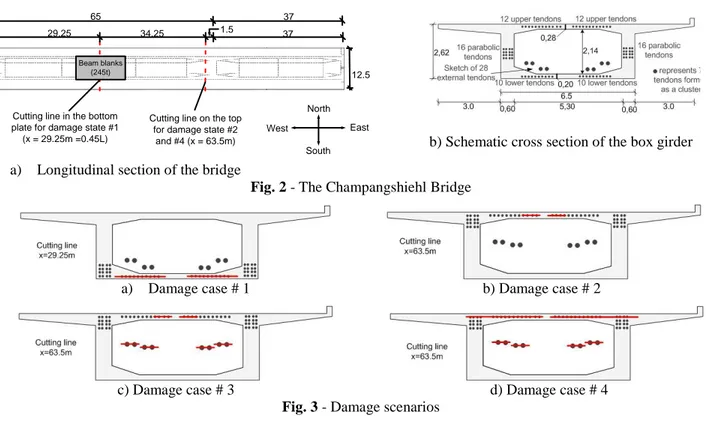
Built in 1966 and located in the centre of Luxembourg, the bridge has a total length of 102 m divided into two spans of 37 m and 65 m (henceforth noted L) respectively (Fig. 2a). It is pre-stressed by 112 steel wires as illustrated in Fig. 2b. Before its complete destruction, the bridge was monitored and a series of damages were artificially introduced as summarized in Table 1. The four damage cases considered are illustrated in Fig. 3a-d.
The measurement setup considered in the present work is given in Fig. 4. Ten sensors were located on each side A and B of the deck (the distance between each sensor is about 10 m). Vibration monitoring under swept sine excitation force and impact excitation were performed on the healthy structure and at each damage state. More detailed descriptions of the bridge can be found in [14].
a) Longitudinal section of the bridge
Fig. 2 - The Champangshiehl Bridge
a) Damage case # 1 b) Damage case # 2
c) Damage case # 3 d) Damage case # 4
Fig. 3 - Damage scenarios 3.2 Feature collection
Vibration responses of the bridge in the healthy state and 4 damaged states were recorded during June 2011. Processing of the data was performed in [9, 14] using the Stochastic Subspace Identification (SSI) method and the Global Polynomial
12.5 Cutting line in the bottom
plate for damage state #1 (x = 29.25m =0.45L)
Cutting line on the top for damage state #2
and #4 (x = 63.5m) 37 29.25 34.25 1.5 65 North South West East 37 Beam blanks (245t)
b) Schematic cross section of the box girder with location of the tendons
Method available in the MEscope Software. For the sake of comparison between different methods and of exploiting statistic damage indexes cited above, features are identified here using the Wavelet Transform. Moreover, in order to broaden false-positive tests that avoid false alarms for undamaged states, data in the healthy condition are enriched and gathered from different days and different excitations. As presented in Figs. 5 and 7, two sections #0 correspond to the impact and then swept sine excitations, respectively, which were performed in two separate days. The damaged states are examined under the swept sine excitations.
Table 1 - Description of the damage scenarios according to the cutting sections shown in Fig. 3
State Damage Percentage cutting (100% equals all
tendons in the defined section cut)
# 0 Undamaged state 0.45L Over the pylon
# 1 Cutting straight lined tendons in the lower part, at 0.45L (20 tendons) 33.7% 0%
# 2 Cutting 8 straight lined tendons in the upper part, over the pylon 33.7% 12.6%
# 3 Cutting external tendons (56 wires) 46.1% 24.2%
# 4 Cutting 16 straight lined tendons in the upper part and 8 parabolic tendons 46.1% 62.12%
Fig. 4 - Location of the sensors on the bridge deck
During the monitoring of the bridge, temperature was also measured outside and inside of the bridge. As all the states were carried out one after the other and so recorded at different days in June, the environmental conditions changed from one measurement set to the other. Fig. 5 displays the ambient temperature (under the bottom plate of the superstructure) as well as temperatures measured at the top and at the bottom of the bridge. For security reason, the temperature monitoring system was removed before the most significant damage #4 so that the temperature was not recorded for the last state.
Fig. 5 – Evolution of the temperature during states #0 ÷ #3 (no data recorded for state #4 )
Modal identification and damage detection were performed in [9, 10, 14] without taking into account temperature variations. It gave the results shown in Table 2 and Fig. 6.
It can be asserted from Table 2 and Fig. 6 that all the damage states are well detected. However, according to these results, state #2 shows a particular behavior: the frequency of mode 1 increases slightly with respect to the healthier states while the frequency of mode 2 exhibits the most important drop. The variation of temperature shown in Fig. 5 may be suspected as responsible for this particular behavior. For damaged state #2, the corresponding ambient temperature does not look unusual
as it is in the same range of the ambient temperature recorded for the healthy state #0; however the temperature at the top of the bridge during state #2 is the highest. This observation is probably the reason why state #2 has a non-conventional behavior compared to the other states. In the following, it will be shown that the proposed methods allow to answer this problem.
Table 2 - Change in the eigenfrequencies (identified by the SSI method)
Healthy D1 f D2 f D3 f D4 f
f1 (Hz) 1.92 1.87 -2.6% 1.95 1.6% 1.82 -5.21% 1.75 -8.85%
f2 (Hz) 5.54 5.45 -1.62% 5.24 -5.42% 5.39 -2.71% 5.3 -4.33%
a) Based on the Enhanced PCA method b) Based on diagonal elements of the flexibility matrix Fig. 6 – Damage detection results obtained in [9, 14]
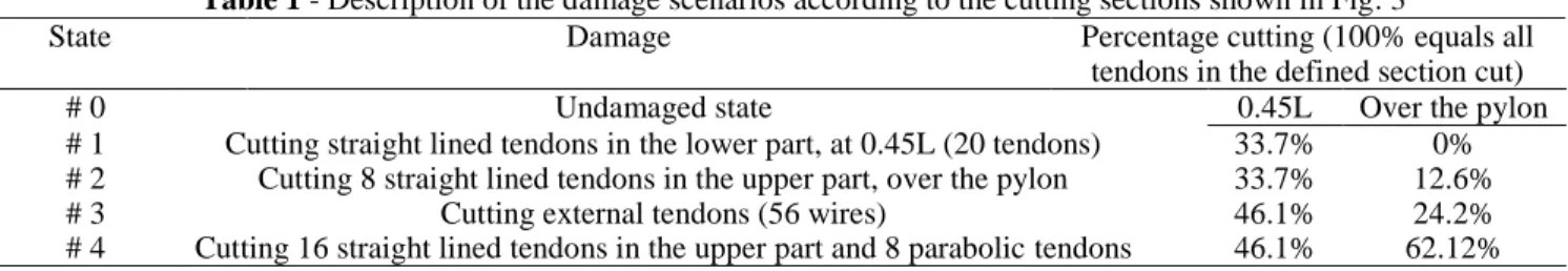
As said before, eigenfrequencies are identified here using the Wavelet Transform (WT) and are chosen as system features. The reason is that the data obtained by WT responses are abundant, so that each eigenfrenquency may be periodically picked up to 300 times for each damaged state, and 2×300 times for the reference state. In total there are 1800 sets of results for all the states. They are plotted in Fig. 7 for the first four modes. The first and the third eigenfrequencies provide a quite clear distinction between different states as the decrease in frequency is monotonous from one state to the others. However, the identification results confirm that the second and fourth eigenfrequencies do not allow to detect damage except in states #3 and #4 for the second mode and only in state #4 for the fourth mode.
Fig. 7 – Eigenfrequencies identified for #0 ÷ #4 3.3 Damage detection using PCA
To maximize useful information for the PCA procedure, all the samples corresponding to the four identified eigenfrequencies are assembled in the feature matrix X according to equation (1). The SVD of X (equation 3) reveals that the first singular
H H H H H H H H D1 D1 D1 D2 D2 D2 D3 D3 D3 D4 D4 D4 0 5 10 15 20 25 30 35 40 45 50 Tests S u b s p a c e a n g le ( °)
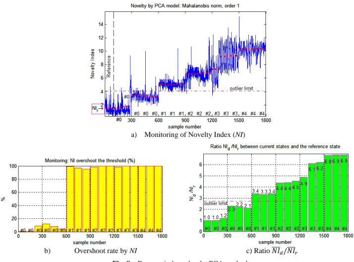
value concentrates about 99% of the energy, which means that only one environmental factor has a significant influence on the four eigenfrequencies. In this case, the environmental factor is the temperature (it is the only one that is noticeable). It means that one principal component is enough to characterize the system dynamics. The other singular values are small and may be attributed to the effect of noise; their influence is so small that they do not affect the diagnostics. Fig. 8 presents the results of the PCA-based detection using the 1 principal component. In this figure, three data sets are considered for each case of damage and six data sets for the reference state. Each data set contains 100 samples. Dotted bold horizontal lines in Fig. 8a give mean values of the Novelty Index (NI) of all the 18 sets of data. The first healthy set is chosen as reference and its mean value is indicated by ̅̅̅̅. The percentage of samples exceeding the outlier limit is given in Fig. 8b and the ratio ̅̅̅̅ ̅̅̅̅ in Fig. 8c.
An overall look at Fig. 8a reveals an interesting result: despite the variation of the NI for the 6 undamaged states #0 (which results from the variation of the eigenfrequencies with the temperature), most of the NI values lies below the outlier limit line. The few samples crossing this line are influenced by other factors (presence of nonlinear effects, noise). Fig. 8a also reveals that all the damage states are detected and well classified in accordance with their levels. Despite the fact that all healthy states are not measured continuously and that their temperature range does not cover every states, consistent results are obtained.
In Fig. 8b, the percentage of NI overpassing the limit is close to 100% for all the damaged states showing that even the smallest damage is clearly detected. In Fig. 8c, the ratio ̅̅̅̅ ̅̅̅̅ is use to exhibit the progression of damage.
a) Monitoring of Novelty Index (NI)
b) Overshoot rate by NI c) Ratio ̅̅̅̅ ̅̅̅̅
Fig. 8 – Damage indexes by the PCA methods 3.4 Detection by KPCA
In this application, the radial basis function is used with the width of Gaussian kernel w = 5. The principal kernel subspace is defined by the first 3 principal components because the first three eigenvalues present above 90% of variance percentage and the next value shows a clear decrease.
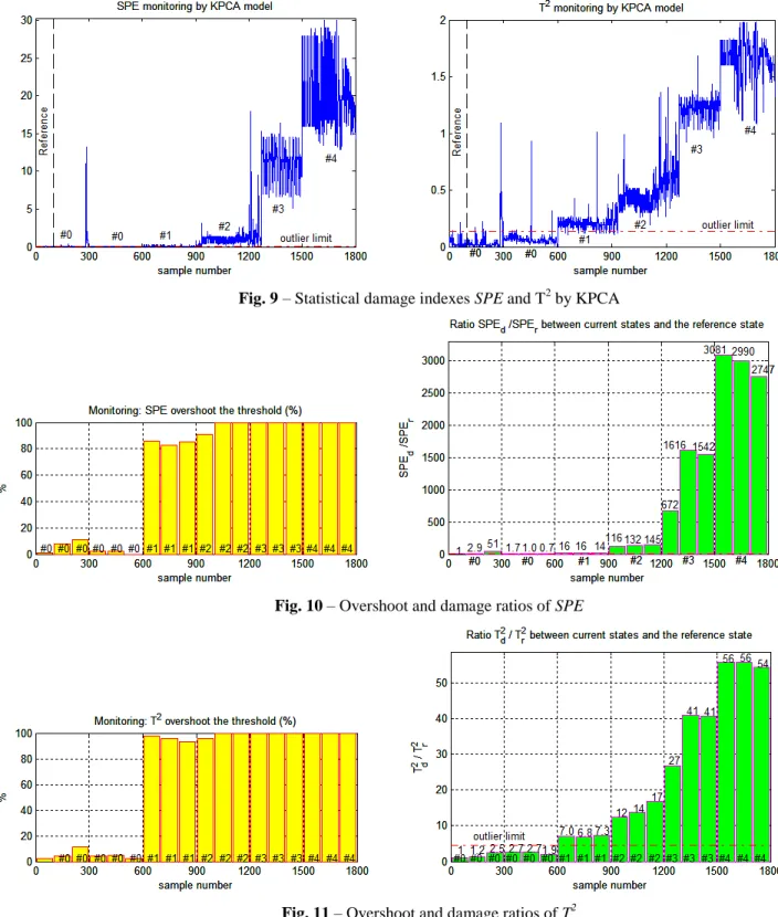
The charts of SPE and T2 indexes are reported in Fig. 9. At first view, the diagnosis is striking by both the charts. By reason of imposing values according to damages #3 and #4, particularly in the SPE chart, more detailed interpretations as presented in Figs. 10 and 11 are necessary.
The comparison between the last two figures reveals that all damages states are completely detected by both SPE and T2 overshoots. As for ratio SPEd/SPEr, it shows two opposed aspects: while state #1 is not detected and alerts occur only from
#2, damages #3 and #4 result in multifold rates. More harmonically, grades perfectly all damaged states, the intact states show regular ratios. There is a clear discrimination between values of intact and damaged states. An explicit improvement with respect to PCA is observed: the values according to the intact states are in the same range for both
̅̅̅̅ ̅̅̅̅ and , however, is much more sensitive to damages as its ratios are weightier. The more damage is important, the more improvement is exclusive.
Fig. 9 – Statistical damage indexes SPE and T2 by KPCA
Fig. 10 – Overshoot and damage ratios of SPE
4. Conclusion
Data recorded from a real concrete bridge are processed by several techniques in this paper. Environmental effects could be removed through PCA and KPCA that eigenfrequencies are considered as features and statistics as damage indexes. Dealt with the same data, this study shows a meaningful improvement with respect to earlier analysis [9, 10, 14] in which damage #2 showed uncommon behaviors (apparent by eigenfrequency, damage index). This uncommonness is cancelled out through the damage indexes used here.
By adopting nonlinear kernel functions, KPCA shows its versatility. Compare to NI (PCA) and SPE, T2 is proven the worthiest damage index in this problem.
The advantage of the detection here is its simplicity. No-environmental measurement is needed. The feature collection is achieved by Wavelet Transform, then PCA or KPCA is used for analysis, they are all very practical and convenient to automation. It is shown that even if reference data is not collected according to a full range of temperature covering other states, the detection is still faithful.
5. Acknowledgment
The author Nguyen V. H. is supported by the National Research Fund, Luxembourg. 6. References
[1]. Ko J. M., Chak K. K., Wang J. Y., Ni Y. Q., Chan T. H. T., Formulation of an uncertainty model relating modal parameters and environmental factors by using long-term monitoring data, Smart Structures and Materials 2003: Smart Systems and Nondestructive Evaluation for Civil Infrastructures, 298, 2003.
[2]. Yan A.-M., Kerschen G., De Boe P., Golinval J.-C., Structural damage diagnosis under varying environmental conditions- Part I, II, Mechanical Systems and Signal Processing 19, pp. 847-880, 2005.
[3]. Deraemaeker, Reynders, De Roeck, Kullaa, Vibration-based structural health monitoring using ouput-only measurements under changing environment, Mechanical Systems and Signal Processing 22, pp. 34-56, 2008.
[4]. Kullaa J., Elimination of environmental influences from damage-sensitive features in a structural health monitoring system, Structural Health Monitoring – the Demands and Challenges, CRC Press, in Fu-Kuo Chang (Ed.), Boca Raton, FL, pp. 742-749, 2001.
[5]. Limongelli M.P., Frequency response function interpolation for damage detection under changing environment, Mechanical Systems and Signal Processing 24, pp. 2898-2913, 2010.
[6]. Kullaa J., Damage detection of the Z24 bridge using control charts, Mechanical Systems and Signal Processing 17(1), pp. 163-170, 2003.
[7]. Reyders E., Wursten G., De Roeck G., Output-only structural health monitoring by vibration measurements under changing weather conditions, Proceedings of the third International Symposium on Life-Cycle Civil Engineering IALCCE, 3-6 October 2012, Vienna, Austria, 2012.
[8]. Nguyen V. H., Golinval J.-C., Damage localization in Linear-Form Structures Based on Sensitivity Investigation for Principal Component Analysis, Journal of Sound and Vibration 329, pp. 4550-4566, 2010.
[9]. Nguyen V.H., Rutten C., Golinval J.-C., Mahowald J., Maas S. & Waldmann D., Damage Detection on the Champangshiehl Bridge using Blind Source Separation, Proceedings of the Third International Symposium on Life-Cycle Civil Engineering, IALCCE’12, pp. 172-176, 2012.
[10]. Mahowald J., Maas S., Scherbaum F., Waldmann D., Zuerbes A., Dynamic damage identification using linear and nonlinear testing methods on a two-span prestressed concrete bridge, Proceedings of the Third International Symposium on Life-Cycle Civil Engineering, IALCCE’12, pp. 157-164, 2012.
[11]. Schölkopf B., Mika S., Burges C.J.C., Knirsch P., Müller K.-R., Smola A., Input space vs feature space in kernel-based methods, IEEE Transaction on Neural Networks 5, pp. 1000-1017, 1999.
[12]. Lee J. M., Yoo C.K., Choi S. W., Vanrolleghem P. A., Lee I.-B., Nonlinear process monitoring using kernel principal component analysis, Chemical Engineering Sciences 59, pp. 223-234, 2004.
[13]. Nguyen V.H., Rutten C., Golinval J.-C., Fault detection in mechanical systems based on subspace features, International Conference on Noise and Vibration Engineering ISMA, Leuven, Belgium, September 2010.
[14]. Mahowald J., Maas S., Waldmann D., Zürbes A., Scherbaum F., Damage Identification and Localisation Using Changes in Modal Parameters for Civil Engineering Structures, Proceedings of the International Conference on Noise and Vibration Engineering, Leuven, Belgium, pp. 1103–1117, 2012.