1
Quantitative temperature monitoring of a heat tracing experiment using
cross-borehole ERT
Hermans Thomas1,2, Wildemeersch Samuel3, Jamin Pierre3, Orban Philippe3, Brouyère
Serge3, Dassargues Alain3, Nguyen Frédéric1.
1
University of Liege, Applied Geophysics, Department ArGEnCo, Engineering Faculty, B52, 4000 Liege, Belgium.
2
F.R.S.-FNRS Research Fellow.
3
University of Liege, Hydrogeology and Environmental Geology, Aquapole, Departement ArGEnCo, Engineering Faculty, B52, 4000 Liege, Belgium.
Corresponding author
Hermans Thomas, University of Liege, Applied Geophysics, Department ArGEnCo,
Engineering Faculty, B52, Chemin des Chevreuils 1, 4000 Liege, Belgium. Tel : +3243669263, Fax : +3243669520, [email protected]
NOTICE: this is the author’s version of a work that was accepted for publication in
Geothermics (53), 14-26. Changes resulting from the publishing process, such as peer review, editing, corrections, structural formatting, and other quality control mechanisms may not be reflected in this document. Changes may have been made to this work since it was submitted for publication. Please cite as
:Hermans T., S. Wildemeersch., P. Jamin, P. Orban, S. Brouyère, A. Dassargues and F. Nguyen. 2015. Quantitative temperature monitoring of a heat tracing experiment using cross-borehole ERT. Geothermics, 53, 14-26. doi:
2 Abstract
The growing demand for renewable energy leads to an increase in the development of
1
geothermal energy projects and heat has become a common tracer in hydrology and
2
hydrogeology. Designing geothermal systems requires a multidisciplinary approach including
3
geological and hydrogeological aspects. In this context, electrical resistivity tomography
4
(ERT) can bring relevant, qualitative and quantitative information on the temperature
5
distribution in operating shallow geothermal systems or during heat tracing experiments. We
6
followed a heat tracing experiment in an alluvial aquifer using cross-borehole time-lapse
7
ERT. Heated water was injected in a well while water of the aquifer was extracted at another
8
well. An ERT section was set up across the main flow direction. The results of ERT were
9
transformed into temperature using calibrated petrophysical relationships. These ERT-derived
10
temperatures were then compared to direct temperature measurements in control piezometers
11
collected with distributed temperature sensing (DTS) and groundwater temperature loggers.
12
Spatially, it enabled to map the horizontal and vertical extent of the heated water plume, as
13
well as the zones where maximum temperatures occurred. Quantitatively, the temperatures
14
and breakthrough curves estimated from ERT were in good agreement with the ones observed
15
directly during the rise and maximum of the curve. An overestimation, likely related to 3D
16
effects, was observed for the tail of the heat breakthrough curve. The error made on
17
temperature can be estimated to be between 10 to 20 %, which is a fair value for indirect
18
measurements. From our data, we estimated a quantification threshold for temperature
19
variation of 1.2°C. These results suggest that ERT should be considered when designing heat
20
tracing experiments or geothermal systems. It could help also to assess the geometrical
21
complexity of the concerned reservoirs. It also appears that ERT could be a useful tool to
22
monitor and control geothermal systems once they are in operation.
3
Keywords: Heat tracing, geothermal system, time-lapse, cross-borehole electrical resistivity 24
tomography, temperature monitoring
25
4 27
1. Introduction 28
Shallow alluvial aquifers constitute potential shallow geothermal energy reservoirs, relatively
29
abundant and easily accessible. In these low temperature systems, groundwater has an average
30
temperature ranging from 5 to 30°C and may be used for domestic or industrial cooling and
31
heating (Allen and Milenic, 2003; Haehnlein et al., 2010).
32
The two main techniques to exploit shallow geothermal energy systems are ground source
33
heat pump (GSHP), which are closed systems with a vertical or horizontal heat exchanger,
34
and groundwater heat pump (GWHP), which are open systems circulating groundwater
35
between production and injection wells. Designing such systems requires a multidisciplinary
36
approach including geological and hydrogeological aspects. The most common approach is to
37
model the system using a coupled groundwater and heat flow simulator. However, such
38
models require estimating parameters governing heat transport such as heat capacity, thermal
39
conductivity and density. Due to a lack of data, authors often have to rely on standard
40
calculation charts, values found in the literature or default values implemented in softwares
41
(e.g. Busby et al., 2009; Lo Russo and Civita, 2009; Liang et al., 2011; de Paly et al., 2012).
42
In-situ tests, such as thermal response tests (Raymond et al., 2011; Mattsson et al., 2008), or
43
laboratory measurements (e.g. Haffen et al., 2013) are sometimes possible but the deduced
44
values may deliver only well-centered information or may not always be representative of
in-45
situ conditions.
46
Thermal tracing experiments are performed for decades in hydrogeology (Anderson, 2005;
47
Saar, 2011). Such experiments are used to improve the characterization of hydrogeological
48
parameters (e.g. hydraulic conductivity or dispersivity), but the same methodologies may be
49
used to study the thermal properties of shallow geothermal systems (e.g. Vandenbohede et al.,
50
2009, 2011; Giambastiani et al. 2012). However, the heterogeneity of geothermal and
5
hydrogeological systems may be too complex to be fully caught by thermal or solute tracer
52
experiments alone (e.g. Brouyère, 2001).
53
In this context, electrical resistivity tomography (ERT) can bring relevant and spatially
54
distributed information both on the heterogeneity of aquifers and on the temporal behavior of
55
tracers. Indeed, ERT has proven its efficiency to image and/or monitor spatial phenomena
56
(Vereecken et al., 2006) such as salt water intrusions (Nguyen et al., 2009; Hermans et al.,
57
2012c), variations in moisture content (Binley et al., 2002), biodegradation of hydrocarbons
58
(Atekwana et al., 2000), salt tracer experiments (Kemna et al., 2002 ; Robert et al., 2012) and
59
heat injection experiments (Hermans et al., 2012b). It was also used in the characterization of
60
geological structures, for example in the exploration of geothermal systems, where
61
hydrothermal fluids may generate high contrasts of resistivity (Pérez-Flores and Gomez
62
Trevino, 1997; Bruno et al., 2000; Garg et al., 2007; Arango-Galván et al., 2011).
63
Besides the characterization of shallow geothermal systems themselves, their impact on the
64
groundwater temperatures in the aquifer may be important since their exploitation yields cold
65
and heat plumes (Molson et al., 1992; Palmer et al., 1992 ; Warner and Algan, 1984) which
66
may influence aquifer properties and groundwater chemistry (e.g. Jesuβek et al., 2013) and
67
microbiology (Brielmann et al., 2009). Haehnlein et al. (2010) pointed out that, if laws and
68
rules exist in some countries to limit the temperature difference caused by the use of
69
geothermal systems, the development of anomalies is rarely monitored. With the growth of
70
the demand for renewable energy, we can expect that regulations will become stricter and
71
controls of installations more common. New monitoring technologies will be needed and ERT
72
may play an important role to monitor spatially, i.e. not only in wells, the variations of
73
temperature in the aquifer. For example, the temperature changes observed on operating
74
GWHP systems (e.g. Vanhoudt et al., 2011) are typically in the range of temperature that
75
could be detected by ERT.
6
ERT aims at imaging the electrical resistivity distribution of the subsurface. Using
77
petrophysical relationships such as Archie’s law, one may recover indirect parameters such as
78
saturation, water electrical conductivity or total dissolved solid content. Bulk electrical
79
resistivity also decreases with temperature (e.g. Revil et al., 1998). In most studies,
80
temperature effects are undesirable and may create artifacts in the interpretation, a correction
81
term is applied to remove the influence of temperature variations (Hayley et al., 2007;
82
Sherrod et al., 2012). Few studies used time-lapse ERT to monitor directly temperature
83
changes (Ramirez et al., 1993 ; Labrecque et al., 1996b), generally in a context quite different
84
from GWHP or GSHP systems.
85
Hermans et al. (2012b) monitored with time-lapse surface ERT a heat injection experiment at
86
a relatively small scale (45 m) and at shallow depth (2 to 4.5 m). Their results show that ERT
87
is a reliable tool to monitor temperature changes and may be a method of choice for the
88
design and the monitoring of geothermal systems. However, the results need to be extended to
89
deeper and more complex, heterogeneous reservoirs, as it will be considered in this paper.
90
ERT-derived temperatures were very close to temperatures modeled using a calibrated
91
coupled groundwater and heat flow and transport model bringing additional constraints on the
92
thermal properties of the aquifer.
93
For deeper reservoirs, the rapid decrease in resolution and sensitivity of surface ERT becomes
94
a major drawback (Caterina et al., 2013). It is then necessary to consider borehole ERT to
95
improve resolution (Perri et al., 2012). For example, Prevedel et al. (2009) installed deep (600
96
to 750 m) borehole electrodes to monitor the migration of CO2 within a storage reservoir
97
(Bergmann et al., 2012). For cross-hole ERT, the results obtained for a specific study are
98
more easily extendable than for surface ERT because resolution patterns are not depth
99
dependent.
7
In borehole ERT, electrodes are located under the ground surface, either fixed at the
outer-101
edge of the casing or mounted on cables with the borehole fluid ensuring the electrical contact
102
with the surrounding rock. In the latter case, borehole fluid is generally more conductive than
103
the rock and may influence resistance measurements (Doetsch et al., 2010). Using time-lapse
104
ERT, the relative fluid effect will be almost similar at each time-step and should be
105
insignificant in inversion results (Nimmer et al., 2008).
106
In this paper, we study the ability of ERT to monitor temperature changes in a heterogeneous
107
aquifer and follow thermal tracing experiments. We pumped water from a gravel aquifer,
108
heated it and reinjected it in a second well, similar to a GWHP system operation.
109
The paper is organized as follows: first, the field site is described; second, the methodology is
110
presented; then, the results of the ERT monitoring are compared with direct measurements in
111
wells; finally, conclusions are presented.
112
2. Field Site 113
The study site is located in Hermalle-sous-Argenteau in Belgium near the Belgian-Dutch
114
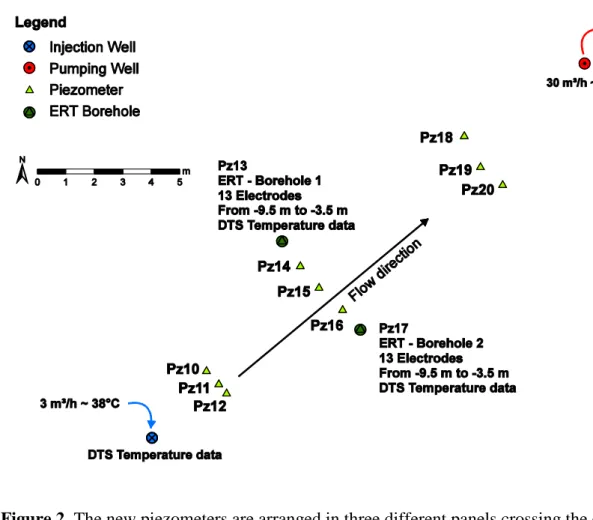
border (Figure 1). It lies on the alluvial aquifer of the Meuse River. A pumping well and 8
115
piezometers were already present on the site since the 1980’s and 11 new piezometers were
116
drilled in June 2012 together with an injection well. They were arranged in three different
117
panels crossing the main flow direction between the injection well and the pumping well in
118
order to study the spatial variability during tracing experiments (Pz10 to 20, Figure 2).
119
Borehole logs enabled to divide the deposits in four different units. The first layer consists of
120
loam and clay with a thickness between 1 and 1.5m. The second layer is composed of gravel
121
in a clayey matrix. The bottom of this layer is found at depth between 2 and 3.2m. These two
122
first layers have little importance in this study because they are located in the unsaturated
123
zone. The water table lies at approximately 3.2m depth, with a very small gradient towards
8
the northeast which is the main direction of flow (Figure 2). The third unit is composed of
125
gravel and pebbles in a sandy matrix. The quantity of sand decreases with depth, whereas the
126
size of the pebbles increases with depth, a vertical variability is thus present. Lateral
127
variability in the grain size distribution of the deposits is also expected in this heterogeneous
128
aquifer, leading to variable hydrogeological parameters. Between 9.7 and 10.1 m, the
129
Carboniferous bedrock composed of folded shales and sandstones is found.
130
In the middle panel, the outer piezometers are screened on the whole thickness of the alluvial
131
aquifer. This is also the case for the injection and pumping wells. Except for the latter, they
132
were equipped with a distributed temperature sensing (DTS) system to monitor the
133
temperature during the experiment (Leaf et al., 2012 and references therein) with a spatial
134
resolution of 0.5m. Pz14 and Pz16 were screened at two different levels, with a 2m long
135
screen between 4 and 6m depth and 1m screen between 8.5 and 9.5m. All other piezometers
136
were screened at two different levels, with a 1m screen between 4.5 and 5.5m depth and a 2m
137
screen between 8 and 10m depth. In the middle of each screened zone, a groundwater
138
temperature logger was placed to monitor the temperature and the pressure during all the
139
experiment.
140
Previous studies have shown that the gravel aquifer is very permeable. Calibrated hydraulic
141
conductivity values were found previously between 1.2 10-1 and 2 10-3 m/s (Dassargues,
142
1997; Derouane & Dassargues, 1998; Brouyère, 2001). With such values, it is possible to
143
inject at a rate much higher than Hermans et al. (2012b) who were limited by the low
144
hydraulic conductivity of fine sands and the small thickness of the aquifer.
145
3. Methodology 146
3.1. Heating and injection procedure 147
9
The experiment consists of an injection and pumping test. The groundwater is pumped from
148
the pumping well, located in the northeastern part of the site, downstream from the injection
149
well. We used a pumping rate of 30 m³/h. Given the high hydraulic conductivity values of the
150
aquifer, the corresponding drawdown is only 5 cm in the pumping well and 4 cm in Pz19 (5 m
151
upgradient from the well). The pumping process ensures that the main direction of flow will
152
cross the three intermediate panels. Pumping was started one day before the beginning of the
153
injection of heated water, far early enough to reach a steady-state flow, and continued after
154
the end of injection.
155
We used a mobile water heater (AQUAMOBIL DH6 system) to heat the water injected in the
156
aquifer. It can work at a maximum rate of 3 m³/h with a difference in temperature of about
157
30°C. Given the high hydraulic conductivity of the aquifer, we decided to inject at this
158
maximal rate. During the injection phase, 3 m³/h of the pumped water were derived in a
159
stocking tank, passed through the water heater and injected in the injection well. The mean
160
temperature of the extracted water at the time of the experiment (October-November 2012)
161
was 13°C. With the maximum injection rate, the temperature of the injected water reached a
162
stabilized mean value of 38°C.
163
Injection started on October 30th and lasted for 1 day, resulting in the injection of 72 m³ of
164
heated water. Using groundwater also for injection, the transformation of ERT results into
165
temperatures will be direct and only require a unique petrophysical relationship. However, the
166
heterogeneity of the aquifer and the advection component make the experimental set-up quite
167
complex.
168
3.2. Petrophysical relationship linking temperature and conductivity 169
The aim of the petrophysical relationships is to quantify the link between bulk electrical
170
conductivity and temperature. Bulk electrical conductivity is generally expressed as a function
10
of porosity, grain size and tortuosity (often joined in a term called formation factor),
172
saturation, fluid electrical conductivity and surface conductivity. In this case, we are
173
interested in the saturated zone (saturation = 1) where the grain size distribution is dominated
174
by gravel with very few fine elements. We can thus neglect the surface conductivity which is
175
very low for coarse grains (Revil and Linde, 2006). With this assumption, the link between
176
bulk electrical conductivity σb and fluid electrical conductivity σf is
177 f b F (1) 178
where F is the formation factor (Archie, 1942). The latter is variable spatially, depending on
179
the lithology. In the case of a monitoring study, we measure bulk electrical resistivity at
180
different time steps and compare it to a reference state, called the background. If we take the
181
ratio of equation 1 between a specific time-step, representing state 2, and the reference
182
background, representing state 1, we have
183 b 2 f 2 b 1 f 1 (2) 184
and the relation is not dependent on the formation factor anymore. In equation 2, σb1 and σb2
185
are determined with ERT after inversion of resistance data and σf1 is either measured on the
186
field directly or deduced from the temperature of the formation water in the aquifer. The only
187
unknown in equation 2 is the fluid electrical conductivity at state 2, which can be expressed as
188 b 2 f 2 f 1 b 1 (3) 189
Through equations 1 to 3, we see that the variation in bulk electrical conductivity in the
190
saturated zone is related to a variation of the fluid electrical conductivity only. The latter can
191
be caused by a change in fluid salinity or by a change in temperature. If we assume that the
11
salinity of the fluid remains constant during the experiment, the water electrical conductivity
193
depends only on temperature.
194
Hermans et al. (2012a) have shown that for long term experiments (storage phase) at
195
relatively high temperature, the link between temperature and electrical resistivity may be
196
more complex, due to precipitation/dissolution effects related to temperature changes, as
197
shown by Robert et al. (2013). However, in this case, the temperature difference is about
198
25°C and should rapidly decrease due to dispersion effects. The variation of salinity with
199
changing chemical equilibrium should be relatively small. If this effect is not negligible, an
200
additional term in equation 5 should be added and calibrated to derive temperatures.
201
In the temperature interval considered in this experiment (10 to 40°C globally, and 10 to 20°C
202
for the panel monitored with ERT), a linear dependence can be assumed between temperature
203
and fluid electrical conductivity (e.g. Sen and Goode 1992 and Hayley et al. 2007 or Hermans
204
et al. 2012b for applications). This relation can be expressed as
205 f , T f f , 2 5 m ( T 2 5 ) 1 (4) 206
where σf,T is water electrical conductivity at temperature T in °C, σf,25 is the conductivity at
207
25°C, considered as the reference temperature (another reference could be chosen as well) and
208
mf is the fractional change in electrical conductivity per degree Celsius at the reference
209
temperature.
210
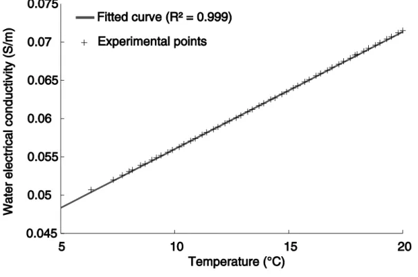
A water sample was taken on the site and relation 4 was verified experimentally in the
211
laboratory (Figure 3). Figure 3 shows the results up to 20°C (temperature encountered in the
212
middle panel), but the trends remains the same until 40°C. Fitting a linear curve to the
213
experimental points, we found mf equal to 0.0194 and the conductivity at the reference
12
temperature (25°C) is equal to 0.0791 S/m. The value for the fractional change per degree
215
Celsius is in the same range as observed by Hayley et al. (2007) and Hermans et al. (2012b).
216
Introducing equation 4 into equation 3, we can express the temperature T (in °C) according to
217
bulk electrical conductivity, water electrical conductivity at the temperature of reference and
218
at the temperature of the background and the fractional change per degree Celsius
219 b 2 , T f 1 f b 1 f , 2 5 1 T 1 2 5 m (5) 220
where σb2,T represents the bulk electrical conductivity at the time-step for which we try to
221
determine the temperature.
222
3.3. Electrical resistivity measurements 223
The two outer piezometers of the middle panel (Pz13 and Pz17 on Figure 2) were equipped
224
with borehole electrode cables with 0.5m spacing. Each borehole has thus 13 electrodes made
225
of stainless steel located from 3.5 to 9.5 m depth. The first electrode is located just below the
226
water table whereas the last electrode is located just above the bedrock.
227
The two boreholes are separated horizontally by 4.5 m. The thickness covered by the
228
electrodes is 6 m. The aspect ratio, i.e. the ratio of the separation between boreholes and the
229
length of the equipped borehole is thus equal to 0.75. This value is often considered as the
230
maximum acceptable value to obtain a sufficient resolution. Optimal resolution is generally
231
achieved with an aspect ratio of 0.5 (LaBrecque et al., 1996b).
232
We used a combination of bipole-bipole (also called AM-BN) and dipole-dipole (AB-MN)
233
configurations as measuring sequence. The first one has a better signal-to-noise, but a lower
234
resolution (Zhou and Greenhalgh, 2000). For bipole-bipole measurements, we measured
235
every possible configuration. For the dipole-dipole, we kept only the cross-borehole
13
measurements, using a dipole spacing ranging from 0.5 to 5m and measuring dipoles sharing
237
one electrode. The complete data set contains 969 possible measurements.
238
We used an ABEM Terrameter LS to acquire the data with an acquisition delay of 0.5s and an
239
acquisition time of 1s. We used a standard deviation limit of 1% on the repeatability error
240
after 3 stacks to filter the data. For almost each time step, we collected both normal and
241
reciprocal measurements to assess the error level on the data. The latter are obtained by
242
swapping current and potential electrodes (LaBrecque et al., 1996a). Acquiring a complete
243
data set took about 45 minutes (normal and reciprocal measurements).
244
The error level was estimated using both the methods of Slater et al. (2000) and Koestel et al.
245
(2008). They both used the reciprocal error to derive a linear relationship between the mean
246
measured resistance Rm (mean between normal and reciprocal resistance, in Ohm) and error e
247
(in Ohm) defined as the difference between normal and reciprocal measurements
248
m e a b R (6)
249
where a is an absolute error (Ohm) and b is a relative error. Slater et al. (2000) considered the
250
envelope curve as error model, which can be considered as conservative, since the mean error
251
is overestimated. Koestel et al. (2008) worked with standard deviation of logarithmic bins to
252
determine the coefficients. This method may result in a mean error model, less conservative.
253
Nguyen et al. (2011) have shown that the noise level characterization is of great importance in
254
time-lapse studies and should always be investigated carefully. If the noise levels are too
255
different between time-steps, it may prevent a quantitative interpretation of monitoring data.
256
If noise levels are almost similar, one should choose a common error model to invert all data
257
sets. We calculated error models for both methods and each time-step. We chose a common
258
error model with an absolute error of 0.002Ohm and a relative error of 0.5%. We tested
14
different error level around these values, with few differences in the final images, both
260
qualitatively and quantitatively.
261
The aim of cross-hole electrical resistivity was to detect the first arrival of the tracer, the
262
maximum temperature reached in the middle panel and, to image vertical and lateral
263
variations in the temperature distribution. Data sets were collected about every six hours
264
during the injection and the day after. For the next days, we increased the time-steps to about
265
18h, with one or two sections per day. The total monitoring time was 6 days, time at which
266
the resistivity distribution had almost returned to the background distribution. For
267
comparison, a DTS system was set in both boreholes to control the temperature directly and
268
assess the ability of ERT to derive reliable temperatures.
269
3.4. Inversion procedure 270
In electrical resistivity tomography, the solution of the inverse problem is non-unique. A
271
common way to solve such inverse problems is to add a regularization constraint to the
least-272
square problem (Tikhonov and Arsenin, 1977). The problem is then to minimize, through an
273
iterative process an objective function of the form
274
2 2
( ) ( f ( ) )
m Wd d m Wmm (7)
275
where λ balances between the data misfit (first term of the right hand side of equation 7) and
276
the model a priori characteristic (second term), d represents the vector containing the data,
277
expressed as the logarithm of measured impedance, m is the model of the logarithm of
278
subsurface electrical conductivity, f(m) is the forward operator, Wd is the data weighting 279
matrix using the reciprocal error as estimate (equation 6) and Wm is a matrix describing an a 280
priori characteristic of the conductivity model. Several forms are possible for Wm, for 281
example to include prior information (e.g. Hermans et al. 2014). The most common method,
15
used in this study, is to penalize roughness to describe smooth model variations
(deGroot-283
Hedlin and Constable, 1990).
284
With time-lapse data sets, we are more interested in the change in electrical conductivity than
285
in the absolute value of conductivity. Generally, the process of inversion is adapted in order to
286
improve inversion results. In this paper, we do not consider coupled inversion of time-lapse
287
ERT data and hydrogeological models (e.g. Irving and Singha 2010). Three main procedures,
288
with several variants, exist to invert for time-lapse ERT data (e.g. Miller et al. 2008), namely
289
independent inversion, time-constrained or reference model inversion and difference
290
inversion. In the first one, inversion results obtained separately are simply substracted, which
291
should eliminate systematic errors but amplify uncertainties in the data. For temporally
292
constrained schemes, a regularization operator is added in the time dimension in addition to
293
the space dimensions, to minimize changes between successive sections (e.g. Karaoulis et al.,
294
2011, 2014). This enables 4D inversions of ERT time-lapse data sets and has already shown
295
to be efficient in tracer tests (Revil et al., 2013). In this study, we used the difference
296
inversion scheme (Kemna et al., 2002) where the problem is formulated in terms of variations
297
for both data and model. Equation 7 becomes
298 2 2 0 0 0 ( ) ( f ( ) f ( ) ) ( ) m Wd dd m m Wm m m (8) 299
where d0 and m0 are respectively the data set and the model corresponding to the background
300
state. The results obtained for the background are thus used as reference for subsequent
301
inversions. This method should reduce the systematic error and provide a faster convergence.
302
(LaBrecque and Yang, 2000).
303
To compare the successive models in the monitoring study, it is important that all data sets are
304
inverted with the same level of data misfit corresponding to the expected noise level. Indeed,
305
over-fitting the data may create artifacts of inversion in the corresponding image, whereas the
16
contrary would results in an over-smoothed inverted section (LaBrecque et al., 1996a). To
307
achieve this, the iteration process is stopped when the root-mean-square (RMS) value of
308
error-weighted data misfit
309 2 R M S ( f ( )) N Wd d m (9) 310
with N representing the number of data, reaches the value 1 for a maximum possible value of
311
λ, corresponding to data fitted to its error level. At each iteration, λ is optimized to obtain the 312
minimum value of εRMS. When, εRMS is inferior to 1, we looked for the unique value of λ that
313
satisfies the data misfit criterion (εRMS = 1).
314
We used the code CRTomo (Kemna, 2000) to invert our data. This code is a 2.5D inversion
315
code; it means that the electrical conductivity distribution is assumed to be constant in the
316
direction perpendicular to the section and that the effect of boreholes themselves cannot be
317
taken into account (Nimmer et al., 2008; Doetsch et al., 2010). Effects caused by boreholes
318
are of more concern when the investigated site is located in high resistive rocks. They may
319
also be, at least partly, avoided with time-lapse inversion. Indeed, we can expect that, if
320
present, 3D artifacts will be compensated because present in both background and monitoring
321
states (Nimmer et al., 2008). However, a possible 3D effect when imaging a contrasting
322
plume, also called shadow effect, is that the plume is imaged even if it is outside the image
323
plane, because the 3D heterogeneity caused by the moving tracer is not taken into account in
324
the 2.5D inversion scheme (Nimmer et al., 2008). This may result in bias in the breakthrough
325
curve, leading to an apparent more diffuse behavior of tracers (Vandenborght et al., 2005).
326
We used a grid with square elements of 0.25 m x 0.25 m, to have two elements between
327
electrodes, extended laterally and in depth for inversion. ERT-borehole 1 is located at
328
abscissa 1 m and ERT-borehole 2 at abscissa 5.5 m on the grid.
17
To assess the quality of the ERT image, we used the error weighted cumulative sensitivity
330
matrix (Kemna, 2000; Caterina et al., 2013). The cumulative sensitivity S is defined as
331 T T d d d i a g ( ) S J W W J (10) 332
where J is the Jacobian matrix and T denotes the transpose operator. S depends on both the
333
distribution of resistivity in the model parameters and the data weighting matrix which
334
depends on the error assessment. A high value of sensitivity for a parameter signifies that a
335
change of its resistivity would strongly influence the data. In contrast, a low value of
336
sensitivity is characteristic of a parameter having less influence on the predicted data. Such a
337
low sensitivity zone will most likely be badly resolved in the inverted section. However, it has
338
to be noted that high sensitivity does not necessarily mean high resolution.
339
4. Results and discussion 340
4.1. Cross-borehole ERT background 341
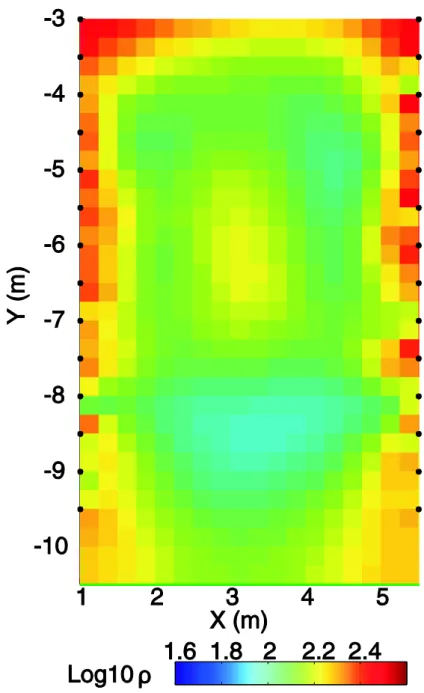
The background image was obtained using equation 7, corresponding to the
smoothness-342
constrained solution (Figure 4). In the zone between the boreholes, we see that the resistivity
343
lies between 100 and 200 Ohm-m, with lower resistivities at the bottom of the section. These
344
resistivity values are characteristic of saturated sand and gravel. The lower resistivity
345
observed at the bottom of the aquifer corresponds with coarser gravel and a lower sand
346
content.
347
The resistivity tends to increase towards the unsaturated zone (above – 3.5m), but there was
348
no electrode in this part of the section (the electrode at – 3 m was modeled but not used for
349
any configuration). However, we do not expect these absolute values to be accurate due to
350
borehole and 3D effects in the inversion (Nimmer et al., 2008).
351
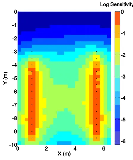
The sensitivity pattern is typical of cross-borehole measurements (Figure 5). The sensitivity is
352
high in the neighborhood of the boreholes and decreases towards the middle part of the
18
section. The sensitivity is lower in two opposite triangles in the upper and bottom part of the
354
saturated zone, due to a smaller coverage of data points in this zone. The lowest sensitivity
355
values are found in the unsaturated zone. The electrical contact through borehole electrodes
356
was not possible because the borehole is not filled with water in this part; no surface
357
electrodes were used to improve the resolution, because the aim is to image temperature
358
changes in the saturated zone. Given the sensitivity values and the aspect ratio, we assume
359
that the chosen configuration is sufficient to monitor temperature changes within the section.
360
4.2. Cross-borehole ERT monitoring results 361
Before looking at inverted data, it is important to qualitatively check if the acquired data
362
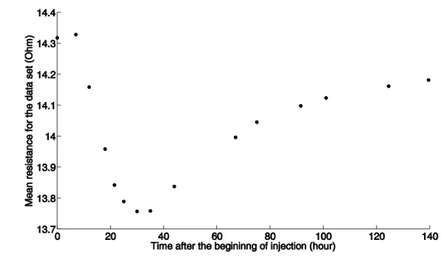
contains some information about the monitored process. We calculated the mean resistance of
363
each data set after removing data with repeatability error higher than 1% (870 points
364
remaining). The mean resistance for the background data set is 14.31 Ohm. The first
365
monitoring set was taken after 7h of injection, the mean resistance slightly increases, but not
366
significantly (Figure 6). This is likely an effect of noise on the data. We can state that
367
temperature changes are too small to influence the measured resistance. The same effect can
368
be observed on individual measurements. The mean resistance then decreases with time to
369
reach a minimum value of 13.76 Ohm after 30 to 35 hours after the beginning of injection,
370
which corresponds to 6 to 11 hours after the end of injection. After the minimum, the mean
371
resistance starts to increase and slightly tends to its initial state, even if it is not totally reached
372
at the end of the monitoring process.
373
Figure 6 can be seen as a qualitative mean breakthrough curve of the heat tracing experiment.
374
It enables to derive two important parameters: the first detected arrival of heat, which occurs
375
between 7 and 12 hours, and the maximum changes, which occurs between 30 and 35 hours.
376
The time-lapse data sets were inverted using equation 8, i.e. the results of Figure 4 are used as
377
a reference and we inverted data differences to derive model perturbations. We kept the same
19
error model for all inversions and we reached a value of εRMS equal to 1 for all inversions,
379
ensuring that all models are fitted to the same level of noise. The results are presented as
380
percentage change of resistivity
381 i B G B G 1 0 0 (11) 382
where ρi is the resistivity of the time-lapse section and ρBG is the resistivity of the background
383
section. A negative value corresponds to a decrease in resistivity (or increase of conductivity)
384
and a positive value corresponds to an increase in resistivity.
385
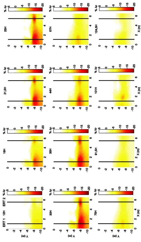
Given the process that is monitored, only negative changes related to an increase in
386
temperature are expected. However, in the inverted time-lapse sections (Figure 7) positive
387
changes of resistivity appear. They are limited in absolute value to +5% in the unsaturated
388
zone which suffers from a very poor resolution, and +3% in the saturated zone. We relate
389
these positive changes to the propagation of data noise in the inversion process (Robert et al.
390
2012). Consequently, we consider that variations in the range -3% to +3% cannot be directly
391
related to temperature variations. They are whitened in the figure. If -3% is the minimum
392
change in resistivity that can be correctly imaged, the limit of detection of ERT for
393
temperature at 13°C for temperature is about 1.2°C (equation 5).
394
The inverted time-lapse sections (Figure 7) show a general behavior of the plume similar to
395
the one observed from the mean resistance. After 7h (not shown), changes in resistance are
396
low and under the level of noise, yielding a section with no changes, i.e. the background
397
model is sufficient to explain the data. After 12h, changes of resistivity about - 5% appear.
398
Then, the decrease in resistivity becomes stronger and reaches a maximum between 25 and 35
399
h. Afterwards, the contrast becomes less strong and after 90 h, almost all changes are below
400
5%. It signifies that their level becomes low to be interpreted quantitatively (close to the limit
401
of detection). However, their spatial distribution is coherent with previous time steps, so it
20
means that the aquifer has not returned to its initial state yet, which is confirmed by the mean
403
resistance.
404
The apparent decrease in resistivity observed in the 101 h section is likely due to an artifact of
405
inversion since it is not physically plausible and does not appear in any other sections. The
406
fact that all other anomalies observed in the sections are recurrent for all time steps and that
407
their amplitude variation follows the trend of classical breakthrough curves validate
408
qualitatively the results of inversion. If some anomalies were related to artifacts of inversion,
409
they would be more randomly distributed for the different time-steps.
410
The advantage of crosshole ERT compared to direct measurements is to provide a spatial
411
distribution of the changes occurring in the aquifer. Figure 7 clearly shows that the changes in
412
resistivity are not homogeneously distributed in the aquifer. Most important changes are
413
observed below -7.5 m depth. This part of the alluvial aquifer is dominated by very coarse
414
gravel with pebbles and a limited amount of sandy matrix, as was observed during drilling.
415
The hydraulic conductivity of the bottom part is higher and the flux is greater, so a major part
416
of heat is flowing in this zone of the aquifer. In the upper part, the convection velocity is slow
417
and the maximum change in temperature is much lower, below the minimum change that
418
ERT can detect. Laterally, we also see variations. The maximum change does not occur in the
419
middle of the section, along the supposed main flow direction. It is located closer to
ERT-420
borehole 1. The resistivity changes are smaller in the middle part, whereas there are a little bit
421
higher in the neighborhood of ERT-borehole 2. Since sensitivity is smaller in the middle
422
section, there is more uncertainty related to those parameters. However, this trend will be
423
confirmed by direct measurements in boreholes (section 4.4).
424
The lateral variations observed in the ERT sections suggest a degree of heterogeneity that was
425
not clearly distinguishable on borehole logs. Zones of preferential flows modify the expected
21
flow direction and result in sections showing a complex spatial behavior. We will see later
427
that these observations are confirmed by direct measurements in borehole.
428
4.3. ERT-derived temperatures 429
For simplicity, we decided to use a constant value of σf1 (equation 5) to transform the ERT
430
images into temperature sections.
431
Equation 4 proposes a linear relationship between water electrical conductivity and
432
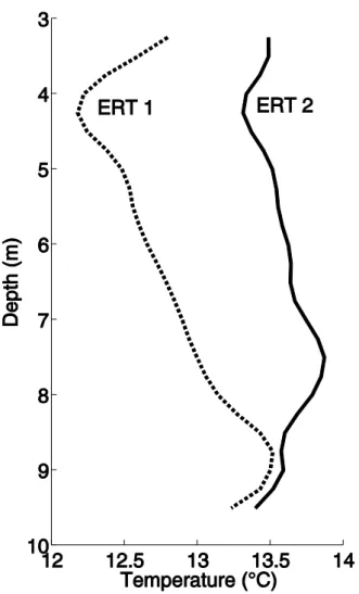
temperature. We thus deduce σf1 based on our direct measurements of temperature. Theyshow
433
that the temperature profile is not constant everywhere in the aquifer and in the ERT section
434
(Figure 8). In ERT-borehole 1, a maximum temperature difference of 1.3°C is observed
435
between the top and the bottom of the aquifer. It is slightly less in ERT-borehole 2. The mean
436
temperature in the two boreholes is also different: 12.8 °C in ERT-borehole 1 (Pz13) and
437
13.6°C in ERT-borehole 2 (Pz17). We took the mean temperature of both ERT-boreholes
438
(13.2°C) and derived with equation 4 a water electrical conductivity of 0.061 S/m. Another
439
solution would have been to interpolate temperatures between boreholes, but it would have
440
made the process more complex without ensuring an improvement of the results.
441
This process has two additional assumptions. First, the specific electrical conductivity of
442
water is constant with time. This was controlled using water samples collected in Pz15 during
443
the test. The changes in the specific conductivity of water are smaller than 1%. The increase
444
in temperature does not seem to favor precipitation or dissolution of minerals. The second
445
assumption is that, at a given temperature, the ratio σf1/ σf,25 (equation 5) is constant in space,
446
or similarly that mf is constant in the whole section. Indeed, if the specific conductivity of
447
water varies in the section, the conductivity at a given temperature varies in the same
448
proportion and the influence on the calculation of temperature is limited. Given the values
449
generally observed in the literature, this assumption is not too severe.
22
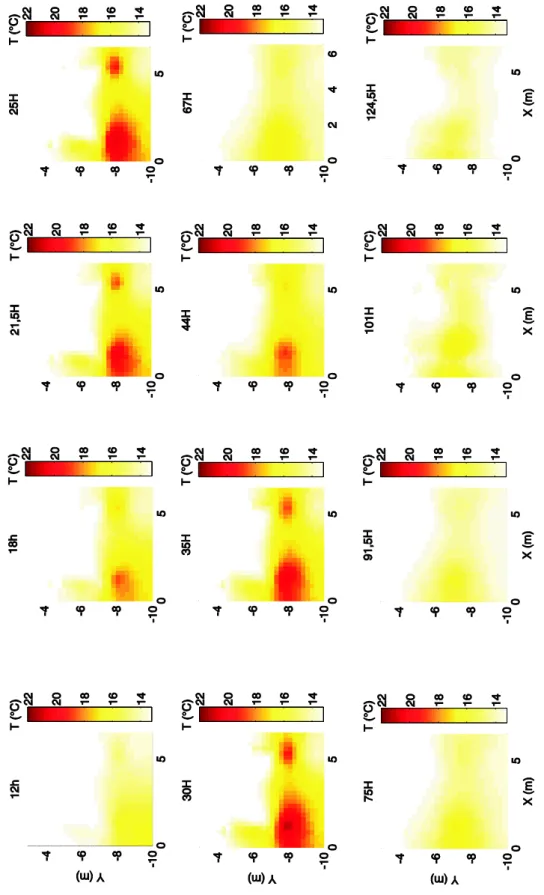
The spatial distribution of temperature (Figure 9) is similar to electrical resistivity changes
451
(Figure 7). Maximum changes of temperature are observed in the neighborhood of
ERT-452
borehole 1, with a maximum temperature of 21°C, which corresponds to an increase around
453
8°C. However, we know that the background temperature in ERT-borehole 1 is slightly below
454
the mean value chosen to draw these sections. Considering the limit of detection of 1.2°C at
455
13°C, temperatures in the range 13.2-14.4°C are only indicative of a small raise in
456
temperature, but the exact value cannot be derived. In addition, we have an error related to the
457
mean water electrical conductivity used in equation 5.
458
4.4. Comparison with direct measurements 459
The layout of the study site enabled to make a lot of direct measurements in piezometers, at
460
different levels in the aquifer. To compare with ERT results, we have DTS measurements in
461
ERT-boreholes 1 and 2, and groundwater temperature loggers at two levels in the three
462
intermediate piezometers Pz14 to Pz16.
463
The quicker arrival of heat in the bottom part of the aquifer (figures 7 and 9) is confirmed in
464
intermediate piezometers (Figure 10 for Pz15). In the upper part, the arrival is very slow and a
465
clear increase in temperature is only visible after 2 days. The oscillations in the signal are
466
disturbances due to sampling of water by pumping from the piezometer. The amplitude of the
467
signal remains very small, below 1°C at the end of the test. Actually, the peak would only be
468
observed after 10 days with an amplitude of about 1.15°C. The same is observed in Pz16 (1°C
469
after 10 days). In Pz14, the change is slightly higher (2°C after 4 days). In the bottom part, the
470
arrival of heat is quicker, after a few hours, with a range of temperature slightly above the
471
limit of detection of ERT. This is totally in agreement with the ERT sections. Spatially, the
472
temperatures observed with ERT are also coherent with direct measurements. The
473
temperatures observed in the bottom part of Pz14 to 16 have a decreasing trend from Pz14 to
474
Pz16, which is also evident from ERT sections where the zone near ERT-borehole 1 is hotter
23
than the middle of the section. As an example, the maximum ΔT in Pz14 is 4.2°C, whereas it
476
is only 2.9°C in Pz15. We can conclude that the qualitative observations on the spatial and
477
temporal distribution of temperature are confirmed by direct measurements.
478
To verify the ability of ERT measurements to quantify temperature, we rely on two different
479
indicators. First, we can draw breakthrough curves at the locations of groundwater
480
temperature loggers to compare the direct measured curve with the ERT-derived curve. This
481
will give insights on the ability to quantify temporally temperature changes. Secondly, we
482
may compare temperature logs at ERT-borehole 1 and 2, to investigate quantitatively the
483
spatial distribution of temperature.
484
Figure 11 shows the breakthrough curves in the bottom part of Pz14 (A) and Pz15 (B) for
485
both direct measurements and ERT. We used the temperatures measured in the corresponding
486
boreholes to determine σf1 in equation 5. For both piezometers, ERT does not detect directly
487
that heat is arrived, because the changes are small, below the sensitivity of the method.
488
However, the rising part of the curve is well resolved with an ERT-derived temperature
489
almost exactly the same as measured directly. The maximum is overestimated, with an error
490
of about 0.5°C in Pz14. The maximum change being 4°C, it represents an error of about
491
12.5%. In Pz15, the fit is less good, but the maximum change is lower and the spatial
492
smoothing of the inversion process may yield an overestimation of the temperature. For both
493
cases, the tail of the curve is overestimated by ERT-derived temperatures. This effect would
494
lead to an overestimation of the thermal dispersivity of the aquifer if ERT results were used
495
alone. This could be related to a 3D effect (shadow effect), because the maximum of the
496
plume, even if not in the section anymore, is still influencing measurements.
497
It must also be kept in mind that the volume investigated by ERT and direct measurements is
498
not the same. Groundwater temperature loggers give a very local measurement inside the
499
piezometer which is itself a singularity inside the aquifer. ERT inversion results give a mean
24
resistivity over the surface of the corresponding cell (here 0.25 cm x 0.25 cm). Another
501
possibility would be an increase of the specific conductivity of formation water due to
502
dissolution of minerals related to the increase of temperature. However, given the quick
503
decrease of temperature when we move away from the injection well, this effect is negligible.
504
This is confirmed by the samples collected in Pz15 which shows an almost constant specific
505
conductivity.
506
Temporally, the results are very satisfactory because the raising part, the maximum and the
507
tailing of the curve are imaged at correct times. In this specific case, the time resolution of
508
ERT is only of a few hours. It signifies that we cannot expect to detect the first arrival with
509
precision. Given the material used, we could achieve a time resolution of half an hour, by
510
reducing acquisition time and acquisition delay which were chosen conservative.
511
The comparison of derived temperatures with DTS measurement in the two
ERT-512
boreholes yields contrasted results and conclusions (Figure 12). In contrast with figure 9,
513
where we used a constant value of σf1, the temperatures measured with the DTS for the
514
background profile were here used to derive a specific value of σf1 for each depth level. In
515
addition, DTS measurements were averaged on the time interval corresponding to the
516
duration of a complete ERT data acquisition. Consequently, the match would be perfect if we
517
would derive temperatures for the background ERT profile using equation 5.
518
In ERT-borehole 1 (Figure 12A), ERT results show the same behavior as observed in Figure
519
7, with higher temperatures in the bottom part of the aquifer, and smaller in the upper part. In
520
contrast, DTS measurements yield an almost constant temperature on the whole thickness of
521
the aquifer. This is a quite surprising observation, because all direct measurements made on
522
the site have shown a clear contrast in temperature distribution between the bottom and upper
523
parts of the aquifer. We think that DTS measurements are influenced by specific borehole
524
conditions and do not reflect the true formation temperature. A possible explanation is that the
25
water suffers from some mixing in and around the well.. ERT measurements, even if
526
influenced by the borehole fluid, are sensitive to the variations outside the borehole itself.
527
This effect may also explain why temperature near ERT-borehole 1 seems to be higher in
528
Figure 9 in the upper part of the aquifer whereas it is not the case in the middle part of the
529
section.
530
In ERT-borehole 2 (Figure 12 B, C and D), the agreement between ERT-derived temperatures
531
and DTS logs is better. It confirms that the hot spot observed near this borehole in Figure 9 is
532
not an artifact of inversion but is related to an increase in temperature. Globally, DTS
533
measurements show slightly less contrast than ERT, maybe also due to borehole conditions as
534
observed in ERT-borehole 1. Quantitatively, ERT-derived temperatures are close to DTS
535
temperatures for the rising and maximum part of the breakthrough curve (Figure 12 B and C),
536
but suffer from an overestimation for the tail (Figure 12 D), as it was observed in Figure 11.
537
Such an effect would be reduced in a storage experiment with conditions of no flow.
538
The comparison of ERT results with direct measurements and their good agreement confirm
539
that the alluvial aquifer is heterogeneous and complex. Instead of a unique heat plume in the
540
middle part of the section, we observed two separated arrivals with a minimum temperature
541
observed in the middle.
542
5. Conclusion 543
The growing demand for renewable energy leads to an increase in the development of
544
geothermal energy projects. Heat storage has become a common energy storage technology
545
and heat is a common tracer in hydrology and hydrogeology. The variation of electrical
546
resistivity/conductivity of water, soils and rocks is a well-known phenomenon and has been
547
studied for several decades. However, the potential of ERT, a method mapping the electrical
26
resistivity of the subsurface, to monitor and quantify temperature was barely approached in
549
the literature.
550
In this paper, we investigated the ability of crosshole ERT to monitor a heat tracing
551
experiment in a complex heterogeneous alluvial aquifer. The studied section was located
552
perpendicular to the main direction of flow to cross the plume of heated water. The results,
553
corroborated by direct measurements in several control piezometers, highlight the ability of
554
ERT to qualitatively monitor the variations of temperature in the aquifer. Spatially, it enabled
555
to map the horizontal and vertical extent of the plume, as well as the zones of maximum
556
temperatures, what would not be feasible with costly and limited direct measurements.
557
If information on the initial fluid conductivity is available, ERT results may be interpreted
558
quantitatively in terms of temperature. The temperatures estimated from ERT were relatively
559
close the ones observed directly during the rise and maximum part of the curve. An
560
overestimation, likely related to 3D effects, was observed for the tail of the breakthrough
561
curve. The error made can be estimated to be between 10 to 20 %, which is a fair value for
562
indirect measurements. The precision of the method may be better in more favorable cases,
563
for example in no or low flow conditions. 3D imaging procedure using more than two wells
564
should also improve the reliability of electrical resistivity monitoring results, yielding a better
565
characterization of temperature distribution.
566
The limit of quantification of temperature changes depends on the noise level observed on the
567
site. ERT requires for an error assessment in order to avoid artifacts in the inverted sections.
568
The higher the noise level, the lower the resolution of ERT to derive temperature changes. In
569
this case, we observed after inversion positive changes of electrical resistivity up to 3% in the
570
saturated zone. Those changes were not physically related to the tracing experiments and
27
enabled us to estimate a limit of quantification for ERT around 1.2°C for temperature
572
changes.
573
In contrast with surface ERT, the resolution of crosshole ERT is not depth-dependent but
574
depends mostly on the aspect ratio, the electrode spacing and the distance to the boreholes. In
575
this case, we achieve an aspect ratio of 0.75 with 13 electrodes. A greater distance between
576
boreholes would require a greater electrode spacing or the use of more electrodes. Standard
577
measurement devices generally accept 24 to 32 electrodes per borehole. Considering an
578
electrode spacing a=0.5 m, we successfully imaged a heterogeneous heat plume with a
579
thickness about 5a and a width of about 4a. The results obtained in this study could be easily
580
extended to other experiment keeping similar parameters. The resolution could even be
581
refined using better aspect ratio or more electrodes. The scale of this experiment could be
582
applied for the control of aquifer thermal energy storage (ATES) located in alluvial plains.
583
For deeper and larger systems, it would require larger distances between electrodes and
584
boreholes or the use of set-up with more than two boreholes.
585
In this experiment, we only achieve a time resolution of a few hours. Our measuring
586
procedure takes about 45 minutes. However, it is possible to reduce acquisition delay and
587
acquisition time of each measurement. It would allow to achieve a time resolution of less than
588
30 minutes. Avoiding the complete collection of reciprocal at each time step would further
589
divide the time to collect the data by two.
590
The results presented in this paper suggest that ERT should be considered when designing
591
heat tracing experiments to derive the parameters governing heat flow and transport in the
592
subsurface or geothermal systems. It should also be used to assess the complexity of the
593
concerned reservoirs. It also appears that ERT could be a useful tool to monitor and control
594
geothermal systems once they are in operation. A proper configuration of ERT wells,
28
depending on the installed configuration, should enable to control the temperature distribution
596
in the reservoir. This may be of crucial importance to better describe the thermal affected
597
zone or assess the possible influence of the system on groundwater chemistry or
598
microbiology.
599
Acknowledgement 600
We would like to thank the associate editor and two anonymous reviewers for their pertinent
601
comments and suggestions which have helped to improve the manuscript. We also thank the
602
F.R.S.-FNRS and the « Fondation Roi Baudouin – Ernest Dubois Award » for their financial
603
support during the PhD of Thomas Hermans.
604
29 606
References 607
Allen, A., Milenic, D., 2003. Low-enthalpy geothermal energy resources from
608
groundwater in fluvioglacial gravels of buried valleys. Applied Energy, 74, 9-19.
609
Arango-Galván, C., Prol-Ledesma, R.M. , Flores-Márquez, E.L., Canet, C.,
610
Villanueva Estrada, R.E., 2011. Shallow submarine and subaerial, low-enthalpy
611
hydrothermal manifestations on Punta Banda, Baja California, Mexico: geophysical and
612
geochemical characterization. Geothermics, 40, 102-111.
613
Archie, G. E., 1942. The electrical resistivity log as an aid in determining some
614
reservoir characteristics. Transactions AIME, 146, 54-62.
615
Atekwana, E.A., Sauck, W.A., Werkema, D.D., 2000, Investigations of
616
geoelectrical signatures at a hydrocarbon contaminated site, Journal of applied
617
geophysics, 44, 167-180.
618
Anderson, M.P., 2005. Heat as a ground water tracer. Ground Water, 43, 951-968.
619
Bergmann, P., Schmidt-Hattenberger, C., Kiessling, D., Rücker, C., Labitzke, T.,
620
Henninges, J., Baumann, G., Schütt, H. 2012 Surface-downhole electrical resistivity
621
tomography applied to monitoring of CO2 storage at Ketzin, Germany. Geophysics 77,
622
B253-B267.
623
Binley, A., Winship, P., West, L.J., Pokar, M., Middleton, R., 2002. Seasonal
624
variation of moisture content in unsaturated sandstone inferred from borehole radar and
625
resistivity profiles, Journal of hydrology, 267, 160-172.
626
Brielmann, H., Griebler, C., Schmidt, S.I., Michel, R., Lueders, T., 2009. Effects of
627
thermal energy discharge on shallow groundwater ecosystems. FEMS Microbiology
628
Ecology, 68, 273-286.
30
Brouyère, S., 2001. Etude et modélisation du transport et du piégeage des solutés en
630
milieu souterrain sariablement saturé, PhD Thesis, University of Liege, unpublished.
631
Bruno, P.P.G., Paoletti, V., Grimaldi, M., Rapolla, A., 2000. Geophysical
632
exploration for geothermal low enthalpy resources in Lipari Island, Italy. Journal of
633
volcanology and geothermal research, 98, 173-188.
634
Busby, J., Lewis, M., Reeves, H., Lawley, R., 2009. Initial geological
635
considerations before installing ground source heat pump systems. Quarterly Journal of
636
engineering geology and hydrogeology, 42, 295-306.
637
Caterina, D., Beaujean, J., Robert, T., Nguyen, F., 2013. A comparison study of
638
different image appraisal tools for electrical resistivity tomography, Near Surface
639
Geophysics,11 (6), 639-657, doi: 10.3997/1873-0604.2013022 .
640
Dassargues, A., 1997. Modeling baseflow from an alluvial aquifer using
hydraulic-641
conductivity data obtained from a derived relation with apparent electrical resistivity.
642
Hydrogeology Journal, 5(3), 97-108.
643
de Groot-Hedlin, C., Constable, S., 1990. Occam’s inversion to generate smooth, two
644
dimensional models from magnetotelluric data. Geophysics, 55, 1613-1624.
645
de Paly, M., Hecht-Méndez, J., Beck, M., Blum, P., Zell, A., Bayer, P., 2012.
646
optimization of energy extraction for closed shallow geothermal systems using linear
647
programming. Geothermics, 43, 57-65. doi: 10.1016/j.geothermics.2012.03.001
648
Derouane, J., Dassargues, A., 1998. Delineation of groundwater protection zones
649
based on tracer tests and transport modelling in alluvial sediments. Environmental
650
Geology, 36 (1-2), 27-36.
31
Doetsch, J.A., Coscia, I., Greenhalgh, S., Linde, N., Green, A., Günther, T., 2010.
652
The borehole-fluid effect in electrical resistivity imaging. Geophysics, 75(4), F107-F114.
653
doi: 10.1190/1.3467824
654
Garg, S.K., Pritchett, J.W., Wannamaker, P.E., Combs, J., 2007. Characterization of
655
geothermal reservoirs with electrical surveys: Beowave geothermal field. Geothermics,
656
36, 487-517.
657
Giambastiani, B.M.S., Colombanii, N., Mastrocicco, M., 2012. Limitation of using
658
heat as a groundwater tracer to define aquifer properties: experiment in a large tank
659
model, Environmental Earth Sciences, published online December 2012, doi:
660
10.1007/s12665-012-2157-2
661
Haehnlein, S., Bayer, P., Blum, P., 2010. International legal status of the use of shallow
662
geothermal energy. doi: 10.1016/j.rser.2010.07.069
663
Haffen, S., Geraud, Y., Diraison, M., Dezayes, C., 2013. Determination of fluid-flow
664
zones in a geothermal sandstone reservoir using thermal conductivity and temperature logs.
665
Geothermics, 46, 32-41.
666
Hayley, K., Bentley, L.R., Gharibi, M., Nightingale, M., 2007. Low temperature
667
dependence of electrical resistivity: Implications for near surface geophysical monitoring.
668
Geophysical research letters, 34, L18402, doi: 10.1029/2007GL031124.
669
Hermans, T., Caterina, D., Nguyen, F. 2014. Case studies of prior information in
670
electrical resistivity tomography: comparison of different approaches. Near Surface
671
Geophysics, in press.
672
Hermans T., Daoudi M., Vandenbohede A., Robert T., Caterina D., and Nguyen F.
673
2012a. Comparison of temperature estimates from heat transport model and electrical
674
resistivity tomography during a shallow heat injection and storage experiment, 1st
32
International Workshop on Geoelectrical Monitoring, Vienna, Berichte der Geologischen
676
Bundesanstalt, 93, 43-48.
677
Hermans T., Vandenbohede, A., Lebbe, L., Nguyen, F., 2012b. A shallow geothermal
678
experiment in a sandy aquifer monitored using electric resistivity tomography. Geophysics
679
77(1), B11-B21, doi:10.1190/GEO2011-0199.1.
680
Hermans, T., Vandenbohede, A., Lebbe, L., Martin, R., Kemna, A., Beaujean, J.,
681
Nguyen, F., 2012c. Imaging artificial salt water infiltration using electrical resistivity
682
tomography constrained by geostatistical data. Journal of Hydrology, 438-439, 168-180,
683
doi:10.1016/j.jhydrol.2012.03.021.
684
Irving, J., Singha, K. 2010. Stochastic inversion of tracer test and electrical geophysical
685
data to estimate hydraulic conductivities. Water Resources research, 46, W11514.
686
Jesuβek, A., Grandel, S., Dahmke, A., 2013. Impacts of subsurface heat storage on
687
aquifer hydrogeochemistry. Environmental Earth Sciences, 69 (6), 1999-2012,
688
doi:10.1007/s12665-012-2037-9
689
Karaoulis, M.C., Kim, J.H., Tsourlos, P.I., 2011. 4D active time constrained resistivity
690
inversion. Journal of Applied Geophysics 73, 25-34. doi:10.1016/j.jappgeo.2010.11.002
691
Karaoulis, M., Tsourlos, P., Kim, J.-H., Revil, A. 2014. 4D time-lapse ERT inversion:
692
introducing combined time and space constraints. Near surface geophysics, 12, 25-34.
693
Doi:10.3997/1873-0604.2013004.
694
Kemna, A., 2000. Tomographic inversion of complex resistivity : theory and
695
application. PhD Thesis. University of Bochum.
696
Kemna, A., Vanderborght, J., Kulessa, B., Vereecken, H., 2002. Imaging and
697
characterization of subsurface solute transport using electrical resistivity tomography (ert)
698
and equivalent transport models. Journal of hydrology, 267, 125-146.
33
Koestel, J., Kemna, A., Javaux, M., Binley, A., Vereecken, H., 2008. Quantitative
700
imaging of solute transport in an unsaturated and undisturbed soil monolith with 3-D
701
ERT and TDR. Water Resources Research, 44, W12411, doi:10.1029/2007WR006755.
702
LaBrecque, D.J., Miletto, M., Daily, W., Ramirez, A., Owen, E., 1996a. The effects
703
of noise on Occam’s inversion of resistivity tomography data. Geophysics, 61, 538-548.
704
doi: 10.1190/1.1443980.
705
LaBrecque, D.J., Ramirez, A.L., Daily, W.D., Binley, A.M., Schima, S.A., 1996b. ERT
706
monitoring of environmental remediation processes. Measurement science and technology, 7,
707
375-383. doi: 10.1088/0957-0233/7/3/019.
708
LaBrecque, D.J., Yang, X., 2000. Difference inversion of ERT data: a fast inversion
709
method for 3-D in-situ monitoring. Proc. Symp. Appl. Geophys. Engng Environ. Problems,
710
Environ. Engng Geophys. Soc., 723–732.
711
Leaf, A.T., Hart, D.J., Bahr, J.M., 2012. Active thermal tracer tests for improved
712
hydrostratigraphic characterization. Ground water, 50 (5), 726-735.
713
Liang, J., Yang, Q., Liu, L., Li, X., 2011. Modeling and performance evaluation of
714
shallow ground water heat pumps in Beijing plain, China. Energy and Buildings, 43,
3131-715
3138. doi: 10.106/j.enbuild.2011.08.007
716
Lo Russo, S., Civita, M. V., 2009. Open-loop groundwater heat pumps development for
717
large buildings: a case study. Geothermics, 38, 335-345. doi:
718
10.1016/j.geothermics.2008.12.009
719
Mattsson, N., Steinmann, G., Laloui, L., 2008. Advanced compact device for the in situ
720
determination of geothermal characteristics of soils. Energy and Buildings, 40, 1344-1352.
721
Miller, C., Routh, P., Brosten, T., McNamara, J. 2008. Application of time-lapse ERT
722
imaging to watershed characterization. Geophysics, 73(3), G7-G17.