& Astrophysics manuscript no. SN_v5 July 10, 2015
Critical analysis
and alternative processing of Type Ia supernovae data
Hauret C. and Magain P.
Institut d’Astrophysique et de Géophysique, Université de Liège, Allée du 6 Août, 19c, 4000 Liège, Belgium Received<date> / Accepted <date>
ABSTRACT
Context.Type Ia Supernovae (SNIa) observations in the late 90’s were the first hints for an accelerated expansion of our Universe. Today, hundreds of objects have been observed and seem to confirm the flatΛCDM model as the cosmological model best representing our Universe.
Aims.We study the SNIa observations gathered in the Union 2.1 and in the JLA compilations. By analyzing correlations and different ways of comparing cosmological models to the data, we bring to light some statistical biases, due to the current way of computing SNIa luminosity corrections for light-curve shape, color and host galaxy mass.
Methods.We suggest an alternative, safer and model-independent methodology to calibrate the luminosity corrections, using only nearby SNIa.
Results.With our recalibrated data, biases are strongly reduced. Moreover, open cosmological models are shown to be favoured over flat models (Ωm,0= 0.26 ± 0.08, ΩΛ,0= 0.66 ± 0.12 for the SCP compilation and Ωm,0= 0.20 ± 0.08, ΩΛ,0= 0.56 ± 0.13 for the JLA one).
Conclusions.The usual method to process SNIa data, i.e. simultaneously determining the parameters of the cosmological model and of the luminosity corrections on the full sample, is prone to bias the data in favour of the assumed cosmology, currently a flatΛCDM model, as well as to bias the cosmological parameters of the assumed model.
Key words. Cosmological parameters – Supernovae : general – Methods : data analysis
1. Introduction
The first evidence for the accelerated expansion of our Universe came in the late 90’s from the study of a specific type of super-novae, Type Ia supernovae (SNIa) (Riess et al. 1998;Perlmutter et al. 1999). These objects are extremely important for cosmol-ogy because they are nearly perfect standard candles, observable over large distances. An astrophysical object is a standard candle if its intrinsic luminosity is known. One can thus easily deduce the distance of such an object by a simple measurement of its apparent luminosity. SNIa are believed to arise from thermonu-clear explosions of white dwarfs in a binary system (Hoyle & Fowler 1960). As these white dwarfs accrete matter from their companions, they grow and reach out explosion conditions when their mass approaches the Chandrasekhar limit (Chandrasekhar 1931). If the very details are still subject to debate, it is easy to figure out that, similar causes leading to similar effects, SNIa present roughly the same luminosity and, thus, make good stan-dard candles.
However, in the last decades, small but significant variations of their peak luminosities have been observed, implying that some corrections have to be applied in order to transform SNIa into genuine standard candles. Correlations have been found be-tween the intrinsic brightness of SNIa, the post-maximum de-cline rate of their light curve (Phillips 1993), their color (Tripp 1998;Riess et al. 1996) and their host galaxy (Kelly et al. 2010;
Lampeitl et al. 2010). In fact, the most luminous objects have the most slowly declining light curves, are the bluest and belong to the most massive galaxies.
Thanks to these correlations, SNIa are nowadays considered as one of our best cosmological tools. They thus have been used for the last 20 years to determine cosmological parameters, lead-ing to the quite general acceptance of the flatΛCDM model (e.g.
Suzuki et al. 2012;Betoule et al. 2014, for recent examples) as the most accurate representation of our Universe to date.
In this paper, we analyse the way the light curve decline rate, color and host galaxy corrections (hereafter called luminosity corrections) are determined and applied. We show that the cur-rently widespread processing of SNIa data produces a significant bias in favour of a particular cosmological model, the flatΛCDM model. We show how it introduces undesirable statistical corre-lations in the data and how these can be avoided.
In Sect. 2, we analyse in detail the methodology currently used to process the luminosity corrections while Sect.3presents the results of our diverse analyses. We study the eventual corre-lations in the data in Sect.3.2and our alternative processing of the SNIa observations is developed in Sect.3.3. Furthermore, a statistical point of view is adopted in Sect.3.4with cosmological fits on binned data. We finally quantify the biases on cosmolog-ical models in Sect.3.5.
2. Current correction method
As previously mentioned, in order to transform SNIa in genuine standard candles, luminosity corrections must be applied. Math-ematically, following the works ofPhillips(1993),Tripp(1998) andSuzuki et al.(2012), we can compute the corrected peak
ab-solute magnitude as:
MB,corr = MB−αx1+ βc + δP(Mstellar< 1010M ) (1) MB being the absolute blue magnitude of the SNIa and MB,corr this same magnitude after applying the luminosity corrections, i.e. the ‘standard candle’ value. x1, c and P are measurements of the SNIa light curve decline rate, color and host galaxy mass (see below), while α, β and δ are parameters which describe the correlations of the peak magnitude to the three aforementioned properties.
First, x1is a measurement of the post-maximum decline rate, related to the so-called stretch correction as the differences in decline rate can also be seen as the stretching of the light curve time axis (Perlmutter et al. 1997a,b). Second, c is generally the observed B − V color of the object at its luminosity maximum (Riess et al. 1996;Tripp 1998). Finally, P is the probability that the SNIa host galaxy is less massive than a threshold fixed at 1010M (Kelly et al. 2010;Lampeitl et al. 2010;Conley et al.
2011). Hence, only the lightest galaxies are found to have a sig-nificant influence on the absolute magnitude of their SNIa.
Initially, MBas well as the α, β and δ coefficients were cal-ibrated on nearby SNIa and the relationships were extrapolated to more distant objects (Phillips 1993;Hamuy et al. 1995;Tripp 1997,1998). However, sincePerlmutter et al.(1999), another de-termination of these luminosity corrections was introduced and became by far the most common way to transform SNIa into standard candles. Indeed, nowadays, MB, α, β, and δ are seen as nuisance parameters and are determined together with the cos-mological parameters by fitting the adopted model (i.e. generally the flatΛCDM model) on the whole Hubble diagram, that is, on high- and low-redshift objects (e.g.Suzuki et al. 2012;Betoule et al. 2014, for recent examples).
That way of computing the luminosity corrections has been widely accepted and hardly ever questioned. However, as already pointed out qualitatively byMelia(2012), this simultaneous fit leads to problematic effects on SNIa data. In fact, when fitting simultaneously the cosmology and the luminosity corrections, the cosmological parameters and the MB, α, β and δ coefficients are not independently determined any more. So, the luminosity corrections on the observational data tend to be somewhat com-pliant with the cosmological model used, as the assumption is made that the adopted cosmology is essentially correct and only its parameters have to be determined. Nowadays, the flatΛCDM model is widely accepted and the present studies on SNIa are predominantly developed to refine the density parameters Ωm,0 andΩΛ,0 values (moreover assumingΩm,0+ ΩΛ,0 = 1). Conse-quently, the data corrections favour this particular model at the expense of any other cosmological model. When corrected that way, the SNIa data do not provide a test of the cosmological model any more, but only a (biased) way of determining its pa-rameters.
3. Evidence of data correlations & alternative processing of SNIa data
3.1. Data sets
In this work, we use SNIa data released in recent compilations, i.e. the Union 2.11 (SCP ; Suzuki et al. 2012) and the JLA2 (Betoule et al. 2014) compilations, containing 580 and 740 ob-jects respectively. When fitted simultaneously with a flatΛCDM
1 http://supernova.lbl.gov/Union/
2 http://supernovae.in2p3.fr/sdss_snls_jla/ReadMe.html
Table 1. Best linear regression slope for original and recalibrated SNIa data
Original data Recalibrated data SCP −0.359 ± 0.052 −0.219 ± 0.049 JLA −0.251 ± 0.040 −0.229 ± 0.037
cosmological model, the resulting best model has a present-day Hubble constant of 70 km/s/Mpc and an actual density parame-ter of matparame-terΩm,0of 0.271+0.015−0.014for the SCP compilation (Suzuki et al. 2012) and of 0.295 ± 0.034 for the JLA one (Betoule et al. 2014). These models will hereafter respectively be called SCP and JLA best models.
3.2. Correlation of luminosity corrections with redshift The search for the best cosmological model implies finding which model best reproduces the variation of the SNIa absolute magnitude MB,corr with redshift z. Thus if the luminosity cor-rections themselves are correlated with redshift, a simultaneous determination of these luminosity corrections and of the cosmo-logical model may results in biasing the data towards the adopted cosmological model.
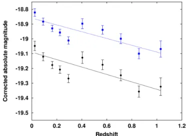
We searched for such correlations by performing linear re-gressions on luminosity corrections (or equivalently absolute magnitudes) versus redshift. A significant slope of the best-fit straight line would imply a significant correlation. The results are shown in the first column of Table1, for the SCP and JLA compilations. The slope is obtained by a fit on the original data, properly taking into account their error bars. The uncertainty on the slope not only includes the contribution from the individual data point errors, but also from their dispersion around a straight line, which is larger than expected based on the individual error bars. These correlations are illustrated by the black plain line on Figs. 1and2 respectively for SCP and JLA data, where SNIa have been grouped in 10 redshift bins for clarity. For both com-pilations, the very significant slopes indicate a clear correlation between SNIa luminosity corrections and redshift.
Part of this correlation is obviously a genuine, physical corre-lation. Indeed, the most luminous SNIa belong to the most mas-sive galaxies (Kelly et al. 2010;Lampeitl et al. 2010) which are more numerous at low redshift. Furthermore, thanks to ultravi-olet and optical photometry observations, it has recently been discovered that SNIa could be separated into two groups with different color properties, low-z SNIa being dominated by one of these groups and high-z ones by the other (Milne et al. 2015). This also probably introduces a correlation between the color of the SNIa and its redshift. This is the very existence of these gen-uine correlations which makes the simultaneous fitting method prone to biasing the data in favour of the adopted cosmological model. Indeed, by forcing the corrected SNIa data to conform to a family of models (namely the flatΛCDM models), the lumi-nosity corrections may be skewed so that the data better fit such models.
3.3. Alternative calibration of SNIa luminosity corrections As we just showed, simultaneous determinations of the cosmo-logical model and luminosity correction are likely to introduce biases. One way to avoid such biases is to return to basics and to use only nearby SNIa to determine the luminosity corrections. We thus determined an alternative and model-independent cali-bration for the luminosity corrections by selecting nearby SNIa
Fig. 1. Linear regressions between absolute magnitude MB,corrand red-shift z of original (black circles and plain line) and recalibrated (blue squares and dotted line) SCP SNIa data. An important variation of MB,corrwith z is particularly observed for original data, sign of an impor-tant correlation between these two SNIa characteristics. When using our recalibrated data, the regression flattens, the difference in slope show-ing the bias introduced by the current methodology to determine SNIa luminosity corrections.
in the Hubble flow (with redshift higher than 0.02 to avoid errors due to peculiar motions of galaxies and lower than 0.09 to stay in this flow where SNIa luminosity distances can still be approx-imated by a linear function of their redshift). Such a calibration is thus independent of any assumed cosmological model.
To face the well-known degeneracy between the MB param-eter and the Hubble constant H0, we fix the latter to the value of Riess et al. (2011), locally determined from a combination of Cepheids and nearby SNIa observations (fitted thanks to the SALT-II light curve fitter (Guy et al. 2007), also used in SCP and JLA compilations) : H0 = 74.8 ± 2.06 km/s/Mpc. In order to safely compare our alternative methodology to the usual one (i.e. simultaneous fit for which the MB, α, β and δ parameters are determined on all SNIa), we determined a different calibra-tion for each compilacalibra-tion, using only nearby objects from the corresponding compilation. Our two best fit calibration parame-ters are summarised in Table2.
With these new luminosity corrections, we perform the same linear regressions (absolute magnitude versus redshift) on the re-calibrated data. The slope values are presented in second column of Table 1 and illustrated (blue dotted line) on Figs. 1 and 2. While the slopes do not significantly differ in the case of the JLA compilation, we observe a significant change when the SCP data are used. The remaining slope is likely due to the genuine physical correlation of SNIa absolute magnitudes with redshift. On the other hand, the change in slope for the SCP data indi-cates the additional bias introduced by the simultaneous deter-mination of the cosmological model and luminosity corrections, a bias which is only marginally detected in the JLA compilation.
3.4. Data correlations evidenced by binning
As we already mentioned, the simultaneous determination of the cosmological model and of the luminosity corrections may force the corrected data to follow the adopted model too closely, thus introducing non-physical correlations between data at different
Fig. 2. Same as in Fig.1with JLA data. Contrary to the analysis made with SCP data, the correlation between MB,corrand z does not signifi-cantly change with recalibrated data.
redshifts. This effect can be emphasised by studying how the data behave when averaged over various redshift bins.
We thus group SNIa in different types and numbers of red-shift bins defined as follows: (i) the N-binning whose every bin gathers the same number N of objects, (ii) the dz-binning whose bins have the same fixed length dz, (iii) the Ndz-binning for which the quantity N ∗ dz is constant for every bin. This latter type of binning was preferred in this study due to its statisti-cal advantages. Indeed, SNIa are not evenly distributed over the redshift range as it is more difficult to observe distant SNIa. The few observed objects at high-redshift are thus statistically less reliable than the numerous low-redshift ones. So with the dz-binning, the high-redshift bins gather much less objects than the low-redshift ones. This could then lead to undesirable statistical bias. On the contrary, the Ndz-binning – as well as the N-binning to a lesser extent – is statistically better suited for an even cov-erage of the full redshift range. It should however be pointed out that our conclusions remain valid, whatever the type of binning. In each of these bins, we compute the weighted mean dis-tance modulus3 ¯µ and its error bar, taking into account both the individual error bars and the dispersion of the data. Then we compare that value to the theoretical distance modulus µthof an hypothetical SNIa whose redshift equals the mean redshift ¯z of SNIa in each bin. The goal of our study being to evaluate the ef-fects of the simultaneous fit of the cosmology and the luminos-ity corrections on the SNIa data, we thus compute the theoretical distance from the cosmological models derived inSuzuki et al.
(2012) and byBetoule et al.(2014), i.e. the SCP and JLA best models defined in Sect.3.1.
Hence, we characterise the fit quality of these latter flat ΛCDM models on the binned data by the calculation of their reduced χ2: χ2 red = 1 ν n X i=1 ¯µ − µth σ¯µ !2 (2)
where ν = n − nparam is the number of degrees of freedom, i.e. the number of bins minus the number of free parameter in the theoretical model (here nparam = 1 because we independently
3 The distance modulus µ is defined as 5 log d
L − 5 where dL is the luminosity distance of the SNIa.
Table 2. Best fit parameters of our two alternative calibrations of SNIa luminosity corrections for each compilation
MB α β δ
SCP −19.111 ± 0.043 0.111 ± 0.027 2.50 ± 0.21 0.063 ± 0.031 JLA −18.8611 ± 0.0078 0.127 ± 0.019 2.79 ± 0.31 0.0141 ± 0.0071
optimise the Hubble constant H0for each binning) and σ¯µis the uncertainty on the mean value of the distance modulus for each bin. The theoretical model provides a statistically satisfactory fit of the data if χ2red' 1. A complementary tool to study a fit quality is the Q probability, defined for a fit with ν degrees of freedom whose χ2has already been evaluated as:
Q ν 2, χ2 2 ! =Γ(ν/2)1 Z ∞ χ2/2 e−ttν/2−1dt (3)
with theΓ function Γ(z) = R0∞e−ttz−1dt(Press et al. 1986). The Q(ν2,χ22) value gives the probability that a χ2 as high as the one measured is compatible with random fluctuations. Hence, mod-els with low Q (typically lower than about 10−3) are excluded by the data while models with Q close to the unity indicate too good to be truemodels (Press et al. 1986).
When we analyse the fit quality of the best SCP model on individual (unbinned) SNIa data of the SCP compilation, we un-surprisingly obtain a good χ2red value of 0.97 associated with a reasonable Q probability of 0.67. This situation is expected be-cause the dispersion component of the SNIa distance modulus uncertainty given by the SCP team is chosen in order to fix the χ2
redvalue to unity (Suzuki et al. 2012). So the fit on non-binned data is (artificially) good.
Statistically, if the errors on the individual data are indepen-dent of each other, the fits of that same cosmological model on these binned data should lead to fits of similar quality (i.e. χ2
red ' 1 and Q ∼ 0.5). The results are shown as black squares on Fig.3, showing the χ2
redand the Q probability values for dif-ferent numbers of Ndz bins4. The SCP best model fits too well the averaged data with χ2
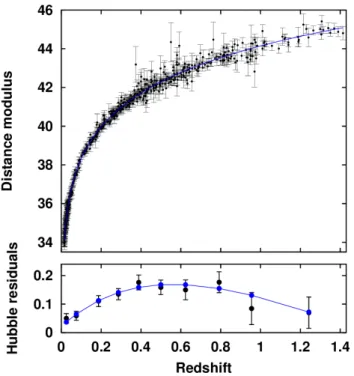
redvalues well under the expected unity and equivalently Q probabilities too close to unity, sign of an obvious overfit of the model to the data. This overfit can easily be visualised on Hubble diagrams of binned data, and is illus-trated on the bottom panel of Fig.4for 10 redshift bins. Indeed, one can notice that, for every redshift bin, the Hubble residuals (and equivalently the luminosity distance) predicted by SCP best model (in blue) invariably stands within the binned one sigma (68.3%) error bars. However, statistically speaking, about one third of these theoretical model points should fall outside the one sigma error bars.
This statistical behaviour indicates that the averaged data do not scatter enough from each other and from the flat ΛCDM model assumed for the calibration. To confirm this hypothesis, we performed the same analysis on our recalibrated data. Its re-sults (χ2
redand Q probability values) are shown as blue triangles on Fig.3which shows much more statistically reasonable values of both χ2
redand Q probabilities. Indeed, the χ 2
red averaged over all trials with 4 to 38 redshift bins amounts to 0.55 ± 0.20 with the original SCP luminosity corrections and 0.84 ± 0.25 with our correction based on low-z SNIa only.
4 As already mentioned, we also analysed the effect of the dz- and N-binnings on the fit quality. The results of the different binning methods being equivalent, we choose to only develop the most statistically sound binning, the Ndz one.
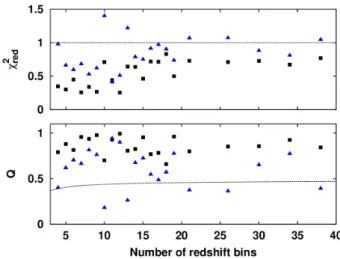
Fig. 3.χ2
red (top) and Q probability (bottom) values for the fit of SCP best model on different Ndz-binnings of the original (black squares) and recalibrated (blue triangles) SCP data. Expected χ2
redand Q values are represented by the dotted lines. For the original data, the χ2
red values are quite under the expected unity while Q stands too close to unity, sign of an overfit, a statistically unusual behaviour of the averaged data. By contrast, when using our alternative calibration of SNIa luminosity corrections, this behaviour is strongly reduced.
Turning now to the JLA compilation, we also found a good fit of JLA best model on unbinned data, with a χ2
red value of 0.98 and an associated Q probability of 0.64. When conduct-ing the same binnconduct-ing analysis as for the SCP compilation, we qualitatively observed the same statistically unusual behaviour of binned JLA data, though to a lower extent, as illustrated on Fig.5. The overfit of JLA best model on original binned data (black squares), while present, is clearly less marked than for the SCP analysis. Nevertheless, when using recalibrated data (blue triangles), one can notice the slightly improved values for both χ2
red and Q probability. The χ 2
red averaged over all trials with 3 to 37 redshift bins amounts to 0.79 ± 0.22 with the original JLA calibration and 0.91 ± 0.28 with our alternative correction.
This analysis shows that the methodology currently used to determine SNIa luminosity corrections introduces correlations between the corrections at different redshifts and biases the data in favour of the assumed cosmology. However, once we calibrate the luminosity corrections on nearby objects only, this undesired behaviour is strongly reduced.
3.5. Impact on cosmological parameters
To quantify the possible biases, we fitted different flat or general ΛCDM cosmological models on the original and recalibrated SNIa data. These genericΛCDM models are described by three parameters, the present-day Hubble constant H0and density pa-rameters for matterΩm,0 and for dark energyΩΛ,0. On Figs.6 and7, we show the one (68.3%), two (95.4%) and three (99.7%) sigma confidence regions in the (Ωm,0, ΩΛ,0) plane that we
ob-Fig. 4. Comparison between the SCP SNIa data and SCP best model (blue line and points), a flatΛCDM model with Ωm,0= 0.271+0.015−0.014and H0= 70 km/s/Mpc. Top : Hubble diagram constructed with all the SNIa data. Bottom : Hubble residuals, i.e. differences between data and an empty cosmological model, averaged over 10 redshift bins (Ndz bin-ning). The binned data do not scatter enough from SCP best model as all the model points invariably stand within the one sigma error bars. This statistically odd behaviour is due to the fact that the cosmological model and luminosity corrections parameters are determined together.
Fig. 5. Same as Fig.3for JLA data. The overfit of JLA best model is present but less marked than for the SCP analysis. Nevertheless, when using recalibrated data, one can notice that the χ2
red and Q probability values are closer to statistical expectations.
tain for the two compilations studied here, using the original (left panels) and recalibrated (right panels) luminosity correc-tions. For each model, the Hubble constant has been optimised in order to provide the best fit of the model to the data.
Naturally, when we use the original SCP data, we recover a model very close to the SCP best model (flat model with Ωm,0 = 0.271+0.015
−0.014 and χ 2
red = 0.971; black square on both
panels of Fig. 6). Indeed, we obtain Ωm,0 = 0.28 ± 0.07 and ΩΛ,0 = 0.73 ± 0.125 (χ2
red = 0.970) shown by the black cross (see left panel of Fig.6). However, when we use our alternative calibration for luminosity corrections, we find a clear discrep-ancy between our best cosmological model (open model with Ωm,0 = 0.26 ± 0.08, ΩΛ,0 = 0.66 ± 0.12 and χ2
red = 0.968; black cross on right panel) and the SCP best model. The latter is excluded at one sigma. The simultaneous fit used bySuzuki et al.(2012) thus obviously tends to bias the SNIa observations in favour of the peculiar cosmology initially assumed, here a flatΛCDM model. Moreover, it introduces a problematic bias in the evaluation of the cosmological parameters. Indeed, even assuming a flat cosmology, our best model obtained after recal-ibration of the luminosity corrections (Ωm,0 = 0.289 ± 0.020 and χ2red = 0.969) differs from the SCP one. In fact, the den-sity parameter for matter from our best flat model is in better agreement with the latest Planck observations (flat Universe with Ωm,0= 0.302 ± 0.012;Planck Collaboration et al. 2015) than the original SCP one.
For the JLA compilation, the situation is slightly different. Indeed, when performing our analysis on original data, our best cosmological model is not a flat one but an open model with Ωm,0 = 0.18 ± 0.09, ΩΛ,0 = 0.54 ± 0.13 (χ2red = 0.977; black cross on the left panel of Fig. 7). Furthermore, the JLA best model (Ωm,0 = 0.295 ± 0.034 and χ2
red = 0.980; black square on both panels), which doesn’t significantly differ from our best flat model (Ωm,0 = 0.292 ± 0.18 and χ2
red = 0.980), is excluded at 1.5 sigma. On the other hand, when using recalibrated data, one can notice that our best model is not significantly modified (Ωm,0= 0.20 ± 0.08, ΩΛ,0 = 0.56 ± 0.13 and χ2red= 1.011; black cross on the right panel), contrary to what happens in the analy-sis of the SCP data.
This difference between the two compilations can be ex-plained by our first analysis and the explanations at the end of Sect. 3.2. Indeed, as already pointed out, the correlation be-tween SNIa corrected absolute magnitudes MB,corr and redshift zis weaker for the JLA compilation than for the SCP one. Thus, while the SCP simultaneous fit produces a strong tendency to bias the SNIa data in favour of the cosmological model assumed (i.e. a flatΛCDM model), this effect is much weaker for the JLA data.
4. Conclusion
Due to the physical correlations between SNIa absolute mag-nitude and redshift, the currently widespread methodology to process the luminosity corrections (i.e. simultaneous fit of lu-minosity corrections and cosmological parameters) is extremely dangerous. Indeed, it can introduce spurious correlations having various impacts over different redshift ranges. The data then tend to become compliant with the assumed cosmology, a flatΛCDM model, making the cosmological test fundamentally untrustwor-thy. This biasing is particularly visible in the SCP compilation, where the additional correlation introduced by the method is es-pecially important, the overfit of SCP best model on binned data is most visible and the modification of the cosmological param-eters is most significant when going from original to recalibrated data analysis.
To avoid these biases, we suggest to go back to a safer model-independent way to process SNIa data, by model-independently cal-ibrating their luminosity corrections parameters on nearby ob-5 The much smaller errors bars in SCP best model are due to them forcing a geometrically flat model.
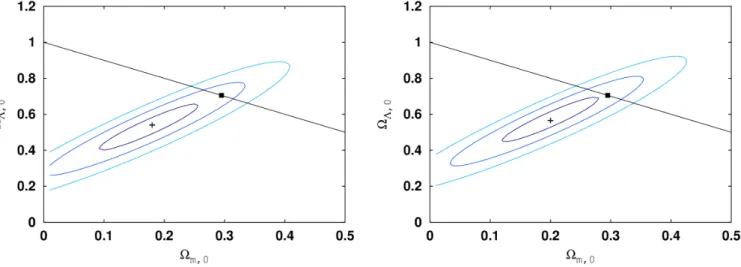
Fig. 6. 68.3%, 95.4% and 99.7% confidence regions in the (Ωm,0, ΩΛ,0) plane of genericΛCDM cosmological models fitted on the original SCP data (left panel) and on data corrected with our alternative calibration of luminosity corrections (right panel). For each cosmological model, the Hubble constant has been optimised in order to obtain the best fit of the data. The best SCP model and our best model are respectively represented by a black square and a black cross, while the full line shows the location of the flat cosmological models, separating the open (below) from the closed ones (above). When using recalibrated data, both the best and the best flat cosmological model significantly differ from the SCP best model.
Fig. 7. Idem as in Fig.6with JLA data. Even with original data, the best cosmological model is an open one, excluding flat models at more than one sigma. When using recalibrated data, no significant discrepancy is observed.
jects. This alternative method allows to more properly evaluate the various cosmological models on the basis of the SNIa ob-servations. These corrected-from-bias data favour an open Uni-verse:Ωm,0= 0.26 ± 0.08, ΩΛ,0 = 0.66 ± 0.12 for the SCP SNIa data and Ωm,0 = 0.20 ± 0.08, ΩΛ,0 = 0.56 ± 0.13 for the JLA ones.
Both ways of calibrating the luminosity corrections assume that the parameters MB, α, β and δ are independent from red-shifts. The traditional way uses all SNIa and has to make prior assumptions onto the cosmological model. Our alternative cali-bration uses only nearby SNIa and avoids any such prior assump-tion. There are more than enough (nearby) SNIa observed to date to calibrate the luminosity corrections independently from the cosmological models and to avoid using methods prone to bias-ing the data.
References
Betoule, M., Kessler, R., Guy, J., et al. 2014, A&A, 568, A22
Chandrasekhar, S. 1931, ApJ, 74, 81
Conley, A., Guy, J., Sullivan, M., et al. 2011, ApJS, 192, 1 Guy, J., Astier, P., Baumont, S., et al. 2007, A&A, 466, 11 Hamuy, M., Phillips, M. M., Maza, J., et al. 1995, AJ, 109, 1 Hoyle, F. & Fowler, W. A. 1960, ApJ, 132, 565
Kelly, P. L., Hicken, M., Burke, D. L., Mandel, K. S., & Kirshner, R. P. 2010, ApJ, 715, 743
Lampeitl, H., Smith, M., Nichol, R. C., et al. 2010, ApJ, 722, 566 Melia, F. 2012, AJ, 144, 110
Milne, P. A., Foley, R. J., Brown, P. J., & Narayan, G. 2015, ApJ, 803, 20 Perlmutter, S., Aldering, G., Goldhaber, G., et al. 1999, ApJ, 517, 565 Perlmutter, S., Gabi, S., Goldhaber, G., et al. 1997a, ApJ, 483, 565
Perlmutter, S. A. et al. 1997b, in NATO Advanced Science Institutes (ASI) Series C, Vol. 486, NATO Advanced Science Institutes (ASI) Series C, ed. P. Ruiz-Lapuente, R. Canal, & J. Isern, 749
Phillips, M. M. 1993, ApJ, 413, L105
Planck Collaboration, Ade, P. A. R., Aghanim, N., et al. 2015, ArXiv e-prints [arXiv:1502.01589]
Press, W. H., Flannery, B. P., Teukolsky, S. A., & Vetterling, W. T. 1986, Numer-ical Recipes. The art of scientific computing.
Riess, A. G., Filippenko, A. V., Challis, P., et al. 1998, AJ, 116, 1009 Riess, A. G., Macri, L., Casertano, S., et al. 2011, ApJ, 730, 119 Riess, A. G., Press, W. H., & Kirshner, R. P. 1996, ApJ, 473, 88 Suzuki, N., Rubin, D., Lidman, C., et al. 2012, ApJ, 746, 85 Tripp, R. 1997, A&A, 325, 871