HAL Id: pastel-00005510
https://pastel.archives-ouvertes.fr/pastel-00005510
Submitted on 20 Oct 2009HAL is a multi-disciplinary open access archive for the deposit and dissemination of sci-entific research documents, whether they are
pub-L’archive ouverte pluridisciplinaire HAL, est destinée au dépôt et à la diffusion de documents scientifiques de niveau recherche, publiés ou non,
Décollement de matériaux viscoélastiques : du liquide
visqueux au solide élastique mou
Julia Nase
To cite this version:
Julia Nase. Décollement de matériaux viscoélastiques : du liquide visqueux au solide élastique mou. Physique [physics]. Université Pierre et Marie Curie - Paris VI, 2009. Français. �pastel-00005510�
UN I VE R S I TA S S A R A V I E NS I S
Th`ese de Doctorat de l’Universit´e Pierre et Marie Curie et de l’Universit¨at des Saarlandes
Sp´ecialit´e : Physique Ecole Doctorale 389
D´
ecollement de mat´
eriaux visco´
elastiques :
du liquide visqueux au solide ´
elastique mou
pr´esent´ee par
Julia NASE
pour obtenir le grade de Docteurde l’Universit´e Pierre et Marie Curie Paris VI -et de l’Universit¨at des Saarlandes
Soutenue le 21 septembre 2009 devant le jury compos´e de
Mme Martine BEN AMAR Pr´esidente du jury
M. Philippe COUSSOT Rapporteur
M. Costantino CRETON Directeur de Th`ese
M. Pascal DAMMAN Rapporteur
Mme Anke LINDNER Directrice de Th`ese
M. Rolf PELSTER Examinateur
M. Ralf STANNARIUS Examinateur
Acknowledgements
I wish to thank first of all Anke Lindner and Costantino Creton who welcomed me as their PhD student and accompanied me during this thesis. Their warm support both personally and scientifically carried me through my time in Paris.
I owe a lot to the interest and inspiration, as well as to the friendship, of my colleagues and co-workers. Besides science, the PMMH and PPMD labs are always a good place to have a coffee!
I thank very much my family and friends and everyone who shared with me all the experiences and adventures Paris offered me.
Debonding of Viscoelastic Materials:
From a Viscous Liquid to a Soft Elastic Solid
In the present experimental study, we investigate the transition in the debonding mechanism when going from a viscous liquid to a soft elastic solid using a probe tack geometry. We have developed a model system consisting of PDMS with differ-ent degrees of crosslinking, ensuring a continuous transition between the material classes. During debonding, a fingering instability with characteristic wavelength evolves. We explain the subsequent coarsening of the pattern for a Newtonian oil by linear stability analysis and identify the influence on the adhesion energy. Over a wide range of properties from liquid to solid, we present a quantitative description of the initially destabilizing wavelength for the observed interfacial and bulk mecha-nisms. We predict the transition between these mechanisms from linear viscoelastic and surface properties. Furthermore, we investigate the debonding quantitatively in terms of adhesion energy and maximum deformation. For interfacial debonding, we are able to explain the speed dependence in the adhesion energy by bulk properties only and confirm thus over two decades in the elastic modulus an existing empiric law. Adapting a recent 3D technique, we visualize for the first time in situ the contact line between viscoelastic material and rigid probe in three dimensions and provide thus direct access to the boundary conditions.
Keywords: adhesion, elastic instabilities, linear viscoelasticity, pattern formation, soft matter, viscous fingering.
D´ecollement de mat´eriaux visco´elastiques : du liquide visqueux au solide ´elastique mou
Dans le cadre de cette th`ese exp´erimentale, nous ´etudions le d´ecollement en g´eom´etrie de probe tack lors de la transition d’un liquide visqueux vers un solide ´elastique mou. Nous avons d´evelopp´e un syst`eme mod`ele (du PDMS `a diff´erents degr´es de r´eticulation), assurant ainsi une transition continue entre ces classes de mat´eriaux. Au d´ebut du d´ecollement, une instabilit´e de digitation avec une longueur d’onde caract´eristique apparaˆıt. Pour une huile newtonienne, nous expliquons le co-arsening des structures lors du d´ecollement par une analyse de stabilit´e lin´eaire, et nous mettons en ´evidence leur influence sur l’´energie d’adh´esion. Pour une large gamme de propri´et´es du liquide jusqu’au solide, nous identifions des m´ecanismes vo-lumiques ou interfaciaux et pr´esentons une analyse quantitative de leur longueur d’onde initiale respective. Nous montrons que le m´ecanisme de d´ecollement est d´etermin´e par la visco´elasticit´e lin´eaire et des propri´et´es de surface. En outre, nous ´etudions le d´ecollement quantitativement par l’´energie d’adh´esion et la d´eformation maximale. Pour le m´ecanisme interfacial, nous arrivons `a expliquer la d´ependance en vitesse de l’´energie d’adh´esion par des propri´et´es volumiques du mat´eriau. Va-riant le module ´elastique sur deux d´ecades, nous confirmons ainsi une loi empirique existante. En adaptant une technique 3D r´ecente, nous visualisons pour la premi`ere fois in situ la ligne de contact entre le mat´eriau visco´elastique et le substrat rigide, offrant ainsi un acc`es direct aux conditions aux limites.
Mots cl´es : adh´esion, digitation visqueuse, formation de structures, instabilit´es ´elastiques, mati`ere molle, visco´elasticit´e lin´eaire.
Abl¨osen viskoelastischer Materialien:
Von der viskosen Fl¨ussigkeit zum weichen elastischen Festk¨orper
Im der vorliegenden experimentellen Studie untersuchen wir den Abl¨oseprozess in einer Probe-Tack-Geometrie w¨ahrend des ¨Ubergangs von einer viskosen Fl¨ussigkeit zum elastischen weichen Festk¨orper. Wir entwickeln ein Modellsystem (PDMS mit verschiedenen Vernetzungsgraden), das einen kontinuierlichen ¨Ubergang zwischen diesen Substanzklassen aufweist. W¨ahrend des Abl¨osens entsteht eine Fingerinstabi-lit¨at mit charakteristischer Wellenl¨ange. F¨ur ein Newtonsches ¨Ol erkl¨aren wir durch lineare Stabilit¨atsanalyse das nachfolgende Coarsening der Strukturen und zeigen ih-ren Einfluss auf die Adh¨asionsenergie auf. ¨Uber einen weiten Bereich der Materialei-genschaften von fl¨ussig zu fest beobachten wir Bulk- oder Grenzfl¨achenmechanismen und pr¨asentieren eine quantitative Analyse der jeweiligen anf¨anglichen Wellenl¨ange. Den ¨Ubergang zwischen diesen Mechanismen sagen wir anhand linearer Viskoelas-tizit¨at und Oberfl¨acheneigenschaften voraus. Ferner untersuchen wir das Abl¨osen quantitativ anhand der Adh¨asionsenergie und der maximalen Verformung. Im Fal-le des Grenzfl¨achenmechanismus erkl¨aren wir die Geschwindigkeitsabh¨angigkeit der Adh¨asionsenergie durch Volumeneigenschaften und best¨atigen damit ein existieren-des empirisches Gesetz. Indem wir eine neue 3D-Technik weiterentwickeln, bilden wir zum ersten Mal in situ die Kontaktlinie zwischen viskoelastischem Material und fes-tem Substrat in drei Dimensionen ab. Damit erm¨oglichen wir einen direkten Zugang zu den Randbedingungen.
Contents
1. General introduction 1
I. Background 7
2. Viscosity, elasticity, and viscoelasticity 9
2.1. Liquids . . . 10
2.2. Elasticity . . . 12
2.3. Viscoelasticity. . . 14
2.3.1. Modeling viscoelastic liquids and solids . . . 14
2.4. Characterization by rheometry . . . 19
3. Theoretical concepts of adhesion 23 3.1. Measuring adhesive properties. . . 23
3.2. Debonding mechanisms . . . 26
3.3. From rheological properties to debonding mechanisms . . . 27
4. Viscous and elastic instabilities in confined geometries 31 4.1. Linear stability analysis . . . 31
4.2. The Saffman–Taylor instability . . . 32
4.2.1. Circular geometry . . . 39
4.2.2. The lifted Hele–Shaw cell . . . 40
4.2.3. Towards non-Newtonian systems . . . 41
4.2.4. Elastic bulk instability . . . 42
4.3. Elastic interfacial instability . . . 43
II. Materials and methods 49 5. Materials 51 5.1. Preparation of the PDMS samples . . . 51
5.2. Characterizing the samples . . . 54
5.2.1. Measurement of the thickness . . . 54
5.2.2. Linear rheological measurements . . . 55
5.2.3. Traction . . . 59
5.2.4. Sol content . . . 59
Contents
5.4. Varying the rheological properties. . . 63
6. Experimental setup and image treatment 67 6.1. The probe tack test . . . 67
6.2. Image treatment . . . 71
III. Debonding of confined viscoelastic materials 73 7. Pattern formation 75 7.1. Introduction. . . 75
7.2. Experimental . . . 75
7.3. Two regimes of debonding . . . 78
7.3.1. Bulk case . . . 79
7.3.2. Interfacial case . . . 82
7.4. Transition . . . 83
7.5. Nonlinear patterns . . . 86
7.6. Conclusion and discussion . . . 88
8. The complete debonding process 91 8.1. Introduction. . . 91
8.2. Experimental protocol . . . 91
8.3. Force-displacement curves . . . 92
8.4. Quantitative analysis of the stress-strain curves . . . 95
8.4.1. Maximum stress . . . 96
8.4.2. Maximum strain . . . 96
8.4.3. Adhesion energy Wadh . . . 97
8.5. Conclusion . . . 102
9. Visualization in three dimensions 105 9.1. Introduction – the need for 3D-visualization . . . 105
9.2. Setup . . . 107
9.3. First results . . . 109
9.4. Conclusion . . . 113
IV. Debonding of Newtonian oils 115 10.The fingering pattern in a Newtonian oil 117 10.1. Introduction. . . 117
10.2. Materials and methods . . . 118
10.2.1. Materials . . . 119
10.2.2. Experimental protocol . . . 120
10.3. The number of fingers in comparison to linear 2D theory. . . 123
10.5. Finger growth . . . 132
10.5.1. Controlled perturbation . . . 137
10.6. Lifting force . . . 139
10.7. A viscoelastic shear thinning liquid . . . 142
10.8. Conclusion . . . 147 Appendix to Chapter 10 . . . 149 V. Conclusions 153 11.Conclusion 155 R´esum´e en Fran¸cais 159 Introduction. . . 159 Mat´eriaux et m´ethodes. . . 160 R´esultats . . . 162 Conclusion . . . 169 Deutsche Zusammenfassung 171
List of Figures
1.1. Surface instabilities in viscoelastic liquids. . . 3
2.1. Different states of a polymer. . . 9
2.2. Shear thinning and shear thickening liquids. . . 11
2.3. Mechanical elements to model viscoelastic materials. . . 15
2.4. σ and γ versus t in Maxwell and Voigt model. . . . 17
2.5. E0 and E00 vs ω for Maxwell and Voigt model . . . . 18
2.6. Schemes of different rheometer measurement geometries. . . 20
3.1. Different techniques to characterize PSA performance . . . 24
3.2. Patterns during the peeling of an adhesive tape . . . 25
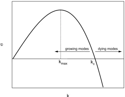
4.1. Schematical view of a Hele–Shaw cell . . . 33
4.2. Sinusoidal deformation of the interface between two liquids . . . 34
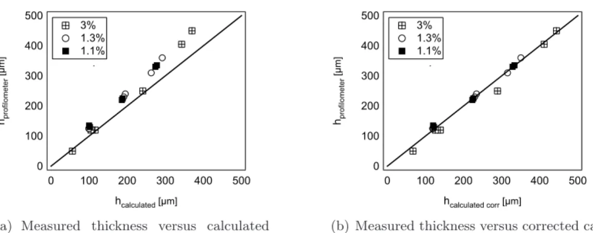
4.3. The growth rate as a function of the wave vector . . . 37
4.4. Destabilization and finger selection in the liner Hele–Shaw cell . . . 39
4.5. Outward fingering in a circular cell. . . 40
4.6. Stress distribution under a rigid punch . . . 43
4.7. Contact instabilities in confined elastic systems. . . 44
4.8. Stability of the contact line in the peeling geometry . . . 46
5.1. Schematical view of the crosslinking process . . . 51
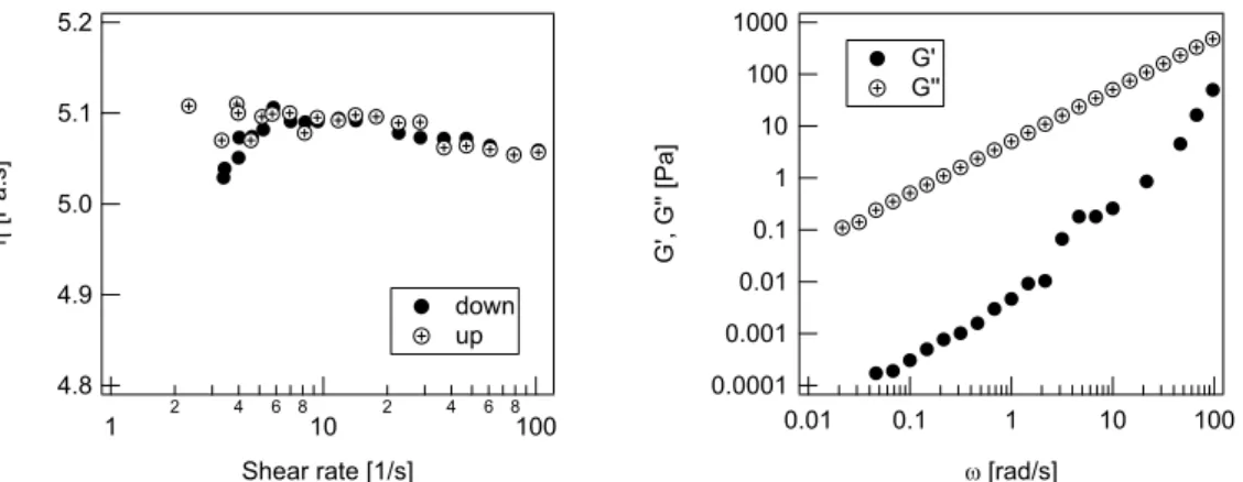
5.2. The sample shape measured in a profilometer . . . 53
5.3. Sample thickness from weighting and from the profilometer. . . 54
5.4. η, G0, G00 for the pure oil . . . . 55
5.5. G0 and G00 versus ω.. . . . 57
5.6. Traction curves . . . 60
5.7. Sol content . . . 61
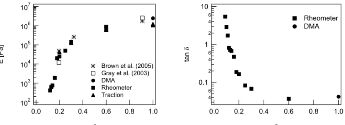
5.8. Moduli and tan δ for some chosen materials. . . . 62
5.9. E and tan δ versus r . . . 63
5.10. G0, G00, tan δ, |η?| versus ω for different T . . . . 64
5.11. G0, G00, tan δ, |G?| versus ω when adding a different oil . . . . 66
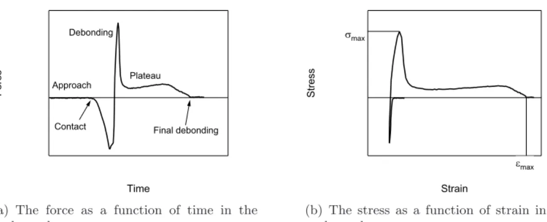
6.1. Typical force-time and stress-strain curves in the probe tack test. . . . 68
6.2. Schematical view of the µ-tack setup. . . 69
6.3. Schematical view of probe polishing . . . 70
List of Figures
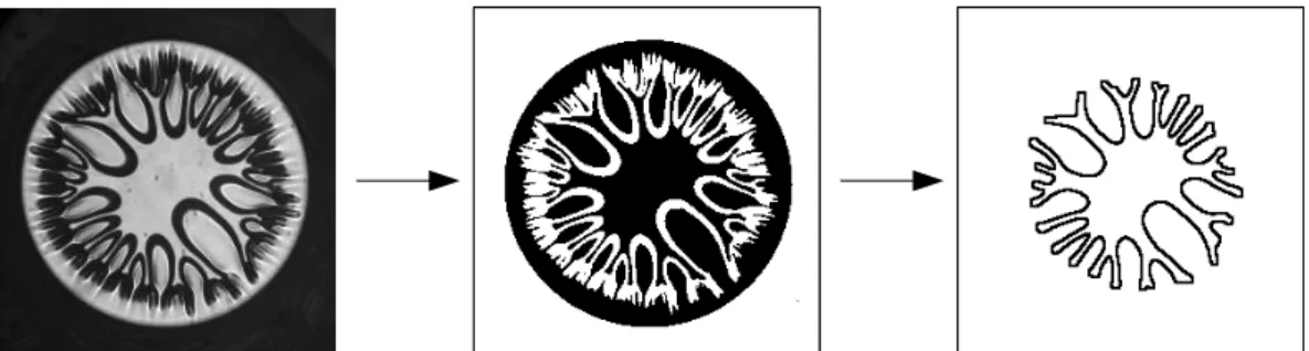
6.5. Image treatment in Igor . . . 72
7.1. Linear destabilization in the bulk case . . . 76
7.2. Linear destabilization in the interfacial case . . . 76
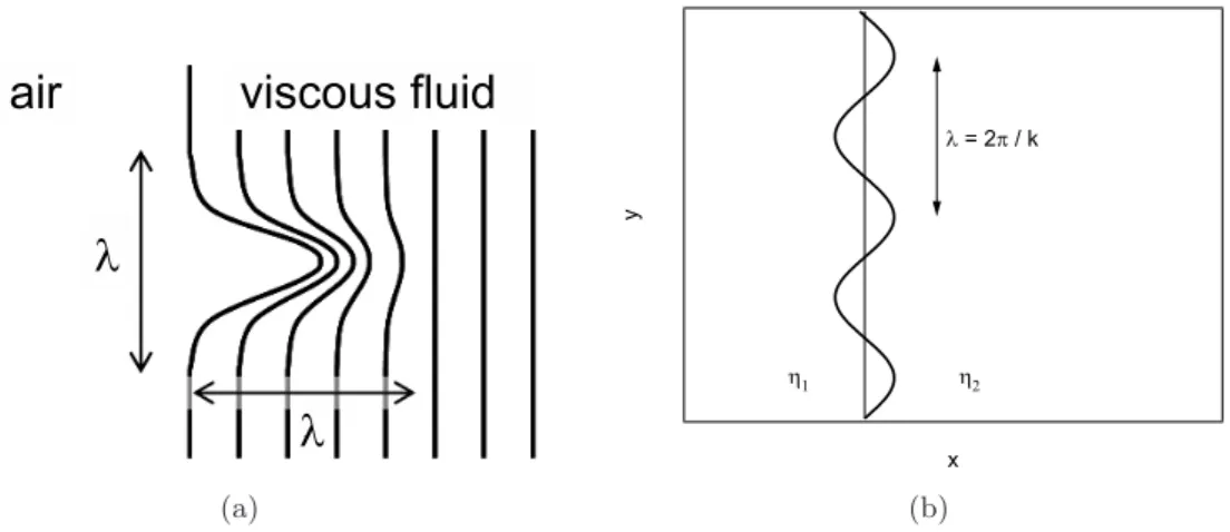
7.3. Schematic view of the wavelength λ. . . . 77
7.4. Side view of fibrillation. . . 78
7.5. Wavelength versus debonding speed. . . 79
7.6. Comparison to the ST theory. . . . 80
7.7. The wavelength for all experiments in comparison to the ST prediction. 82 7.8. Lambda versus film thickness . . . 83
7.9. Mechanism map . . . 85
7.10. λ compared to the ST prediction . . . 86
7.11. Top view images of the cohesive debonding of a pure viscous oil . . . . 86
7.12. Top view images of the debonding of a viscoelastic material . . . 87
7.13. Top view images of the debonding of an elastic material . . . 87
8.1. Typical stress-strain curves of the different materials . . . 93
8.2. Comparison of the stress-displacement curves for different materials . . 94
8.3. Maximum strain versus E . . . 96
8.4. Adhesion energy versus E . . . 97
8.5. Wadh compared to the scaling in the Newtonian case . . . 99
8.6. Wadh versus v for interfacial debonding. . . . 100
8.7. Wadh versus Eb²2max . . . 101
8.8. Wadh/ tan δ versus ω for predominantly elastic materials. . . . 102
9.1. Peeling of a commercial tape from different substrates . . . 105
9.2. Large strain simulations of the debonding of a soft elastomer. . . 106
9.3. Schematic of the 3D-setup of Yamagutchi et al. . . . 107
9.4. The 3D visualization technique, schematical view and setup. . . . 108
9.5. 3D snapshots of interfacial and bulk fingering. . . . 110
9.6. Shape of the contact line for different materials. . . 111
9.7. Estimated contact angle, r = 0.16.. . . 112
10.1. Viscosity versus shear rate . . . 119
10.2. Viscosity versus temperature . . . 120
10.3. Top view of the ST instability in the LHSC . . . 121
10.4. Superposition of the contact lines for different t . . . 122
10.5. N versus t0, comparison to prediction from linear theory . . . . 124
10.6. Growing and dying fingers . . . 125
10.7. Ngrow versus t0, comparison to linear theory . . . 126
10.8. N versus t0, gap width color code . . . . 127
10.9. N versus t0, confinement color code . . . . 128
10.10. Images at τ0= 3.0 × 10⁻⁵ and τ0 = 4.5 × 10⁻⁶ . . . 130
10.11. Nall and Ngrow versus t0 at three different τ0 . . . 131
10.13. Dimensionless perimeter versus dimensionless time . . . 133
10.14. Growth rate and most unstable wave vector at t0 = 0. . . . . 135
10.15. Comparison of the contact line in experiment and simulation. . . 136
10.16. N versus t0 from simulations . . . . 137
10.17. Mask for soft lithography. . . 138
10.18. Images of a cured polyurethane pastille . . . 138
10.19. Force versus strain . . . 140
10.20. F versus t0 from literature . . . . 141
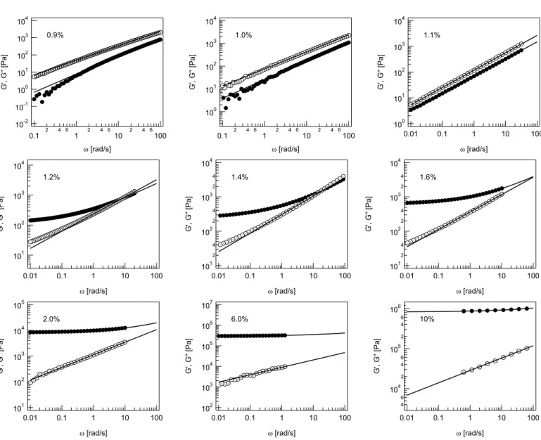
10.21. Viscosity of Carbopol solutions . . . 142
10.22. G0 and G00 versus ω for the 1% Carbopol solution. . . . . 143
10.23. Debonding of 0.1% Carbopol solution . . . 144
10.24. Debonding of 1.0% Carbopol solution, I . . . 144
10.25. Debonding of 1.0% Carbopol solution, II . . . 145
10.26. N versus t for Carbopol . . . 147
10.27. Comparison of experiment, 2D, and 3D theory . . . 151
1. General introduction
The experience of gluing or debonding two bodies is common in everyday life. A large industry is developing and improving the different kinds of glues and adhesives, which are of great importance as well in industrial applications as in workaday life. So-called pressure sensitive adhesives (PSA), are adhering to a substrate upon application of light pressure, and can ideally be detached without leaving traces. The adhesion is generated solely by van der Waals forces, covalent bonds are not involved. Widely spread applications of PSAs are tapes and labels.
PSAs consist of quite complex materials. They have to be liquid enough to form a good contact between two (rough) surfaces one wants to glue together; at the same time, they have to resist strains that occur during debonding. In the last years, much fundamental work was done to understand better the mechanisms of the debonding process. It has been investigated in terms of performance, reflected in quantities such as the adhesion energy or the maximum deformation before complete debonding. Much interest was shown as well to the structures formed during debonding, like cavities or air fingers. These patterns are observed in peel tests as well as in tensile deformation tests.
In the investigation of the patterns as well as in the quantitative analysis of the adhesive performance, the theoretical concepts are well-known for the limiting cases in the material properties. That is, the cases of Newtonian liquids and of elastic solids are well-established, however, the situation is more complex in the crossover region between those limits. To obtain PSAs with good performance, their properties have to be chosen in this crossover region. PSA are thus very complex viscoelastic materials that show simultaneously liquid and solid properties.
Viscoelasticity is a very general property exhibited by many different condensed matter systems, solid or liquid-like. In this work, we are dealing with materials where the elasticity is of entropic origin. Systems such as viscoelastic fluids, more or less crosslinked polymer melts, and polymer networks up to rubber-like materials are typical examples. For these systems the transition from a more liquid-like to a more solid-like behavior can occur very differently depending on the characteristics of the material, as the length of the polymer chains, the number and the nature of crosslink points, or the applied time scale or temperature.
A polymer melt consisting of long polymer chains shows elasticity even in the absence of chemical crosslinks. This elasticity originates from entanglements of the polymer chains that act, at short time scales, as crosslink points. At longer timescales, the polymer chains can slide along each other and the behavior is liquid-like. Therefore, an entangled polymer melt acts like a typical Maxwell fluid: it displays a liquid-like behavior on long time scales and a solid-like behavior on short
Chapter 1. General introduction
time scales. When one starts to crosslink such a melt, the elastic plateau value changes little, as the entanglements are replaced by chemical crosslinks. The re-laxation time of the material increases however strongly and it becomes elastic at larger and larger timescales. Typical PSAs are imperfect polymer networks that are swollen with polymer chains of different length. They are characterized by a wide spectrum of relaxation times, maintaining an almost identical level of viscoelasticity over a wide temperature range. Rubbers or elastomers are characterized by their unique ability to extend to several times their size and recovering their initial shape with (almost) no hysteresis.
When debonding a thin layer of these viscoelastic materials from a substrate, dif-ferent mechanisms are observed. The modification of the debonding mechanism as a function of the viscoelastic properties has been noted by several researchers, but the existing studies have focused on specific, rather narrowly defined systems such as en-tangled polymer melts of linear chains [65,102,63,11,89], polymer melts containing hydrogen bonds [96], Newtonian or lightly viscoelastic fluids [93, 40,113], complex networks resembling commercial PSAs [76, 130,38,32], or well crosslinked rubbers [48, 77, 2]. Many researchers noted the importance of the viscoelastic properties on the adhesive behavior in general [17, 114], and more specifically on the exis-tence and frequency dependence of sharp transitions in mechanisms from cohesive to interfacial failure and from fibrillar deformation to failure by crack propagation [39,49,45,28,69]. Most of the results obtained in these studies have been discussed from the mechanistic point of view [108] or relating the rheology with adhesive be-havior [44]. On the theoretical side, the early work in solid mechanics, which focused on crack propagation in viscoelastic materials [80], has been followed by the insights of de Gennes and coworkers on the modeling of a propagating viscoelastic crack in the bulk or at the interface [34,35,70,101]. Yet a continuous description of adhe-sion from the Newtonian fluids (sticky honey for example) to the adheadhe-sion of elastic rubber has never been investigated within the same material family.
Pattern formation, beside the role it plays in debonding, is also interesting from a more general point of view, as it can be observed in a large variety of systems. It occurs when a so-called homogeneous ground state becomes unstable against small perturbations. The system then passes into a new state, and the formation of pe-riodic patterns ensues. This phenomenon is widely spread in nature; from cloud formation and patterns on animal coats to chemical reactions, pattern formation is a very rich and complex subject. Figure 1.1 reveals the beauty of the resulting structures in two cases. On the left side, we see the instability on a thread of a visco-elastic fluid [100]. The initially straight borders of the jet become unstable towards a sinusoidal deformation whose amplitude is growing in time (Rayleigh–Plateau
in-stability). On complex fluids, droplets on a string are formed at later times. The
instability on a vertically shaken fluid layer (Faraday instability) is shown in figure
1.1(b)(taken from reference [117]). Vertical shaking results in an oscillatory modu-lation of the vertical acceleration. Above a certain shaking frequency and amplitude, the liquid layer develops beautiful periodic patterns of different complexity. Here
(a) Rayleigh–Plateau instability on a viscoelastic thread. The amplitude grows in time (from the left to the right), and then
develops into groups of droplets [100].
(b) Faraday instability: local-ized stationary surface patterns
of harmonic hexagons [117].
Figure 1.1.: Surface instabilities in viscoelastic liquids.
we see stationary hexagons.
Recently, the patterns that are formed during tensile deformation of thin layers in confined geometries have attracted much interest. We consider in this thesis the case of a viscoelastic material confined between two plates which are subsequently separated. Air penetrates from the edges and leads to the formation of bulk or interfacial fingers. The bulk fingering instability is well described by the classical
Saffman–Taylor instability, where a less viscous liquid pushes a more viscous liquid
in a confined geometry [98,104, 87, 40, 93, 75, 10]. Some studies have focused on complex or yield stress fluids [40, 10, 9], ferromagnetic fluids [85], pastes [71], or considered the role of the substrate [110]. However, instabilities are equally known for elastic materials. A surface instability of a thin layer of a purely elastic material with undulating crack front has been observed experimentally and explained theo-retically [1,79,42,47,105,46]. Shull et al. [109] and Webber et al. [118] described a bulk instability for elastic gels.
The transition from the liquid to the solid state is currently a subject of strong interest. The transition between a viscous liquid and a glassy material has been investigated in references [54, 128, 125]. Very recently, Arun et al. performed ex-periments where they approached a flat plate to a thin layer of different viscoelastic materials in an electric field [7]. A change in the wavelength of the resulting surface instability revealed the transition between liquid and solid behavior. However, no systematic study of the pattern formation during tensile deformation of a viscoelas-tic material focusing on the respective role of the liquid and elasviscoelas-tic properties over a wide range of material properties has been undertaken so far.
In this thesis, we investigate here a continuous transition and a large range of prop-erties within one system using a model family of Poly(dimethyl siloxane) (PDMS) with different degrees of crosslinking. We study this transition both in terms of initial pattern formation and in terms of adhesive properties during the highly non-linear
Chapter 1. General introduction
debonding process over the whole range of viscoelastic properties. Such a study contributes to a better understanding of the instabilities observed in viscoelastic materials, which are important for industrial applications. It is also of importance for any theoretical treatment aiming to bridge the gap between the different for-malisms that apply to viscous liquids and elastic solids.
This thesis is divided into four parts. The first part overviews the theoretical background. In Chapter2, we recall the basic principles of viscosity, elasticity, and viscoelasticity, and explain the concepts of rheometry. The focus of Chapter3 lies on adhesion and adhesives. The principles of linear stability analysis are introduced in Chapter 4, and examples for pattern formation in liquids and solids are given.
In the second part, we characterize in detail the PDMS model system, mainly by rheometry, (Chapter5) and we present the “probe tack” setup (Chapter 6).
In the third and forth part, we present the results we obtained in this thesis. Chapter 7 investigates in detail the initial pattern formation during debonding. In the probe tack geometry, we observe an initially circular, smooth contact line be-tween air and viscoelastic material. Soon, the contact line is oscillating and becomes instable. The amplitudes of the oscillations start to grow, and air fingers evolve. We investigate the wavelength of the initial destabilization. Dependent on the mate-rial properties, we identify an interfacial regime, where air fingers propagate at the interface between probe and PDMS, and a bulk regime, where the PDMS bulk is deformed and fingers are formed in the volume. In both cases, we predict quanti-tatively and qualiquanti-tatively the wavelength in agreement with theory. Additionally, we propose an empiric parameter that determines the transition between bulk and interfacial regime. These results have been published in 2008 [81].
In Chapter 8, we investigate the complete debonding process in terms of stress-strain curves. We describe the change in the curve shape as the viscoelastic proper-ties of the material vary and identify clearly three different debonding mechanisms. For very weakly crosslinked materials, we observe a cohesive bulk mechanism, where the complete fingering process takes place in the volume. For intermediate degrees of crosslinking, the debonding is initiated in the bulk and then becomes interfa-cial. For well crosslinked materials, the debonding is purely interfacial without bulk deformation. Quantitatively, the change in the curve shape is reflected in the two quantities adhesion energy and maximum deformation before debonding. For the well crosslinked materials we investigate in greater detail the adhesion energy and explain its speed dependence in terms of viscoelastic bulk properties.
A novel visualization technique is presented in Chapter9. Adapting a recent 3D-technique that is based on the total reflection in a prism [122], we visualize for the first time directly the contact between probe, air, and viscoelastic material in three dimensions. In this way, we estimate the contact angle and are able to determine the boundary conditions of the advancing contact line in situ.
A detailed study of the viscous fingering instability during the debonding of a Newtonian oil completes this work (Chapter 10). We investigate the coarsening of the fingering pattern as the probe is pulled away. We divide the air fingers into
growing fingers, which are moving towards the center of the probe, and dying fingers, which are fixed at their position. We show that the number of growing fingers is very well described by linear stability analysis. Furthermore, we investigate the finger amplitude and the force that is needed to debond the probe, and find that both quantities depend on the confinement.
The last part concludes this thesis. An extended r´esum´e in German and French can be found at the end of this manuscript.
Part I.
2. Viscosity, elasticity, and viscoelasticity
The materials we used in this study are all based on polymers. The term polymer denotes a large class of materials, including such diverse substances as plastics, rub-ber, DNA, and cellulose. Their common feature is that they are macromolecules, made of repetition units (monomers), which are typically connected to each other by covalent chemical bonds. Polymers in general show very complex behavior. One of their most striking properties is that they behave as a brittle solid, an elastomer, or a liquid, depending on the temperature and on the experimental time scale. A distinction is made between viscoelastic liquids and viscoelastic solids. Viscoelastic liquids are polymer melts in which the polymer chains can flow freely. At intermedi-ate times, the elastic character is predominant, but at long times, they behave like liquids. This behavior is in contrast to viscoelastic solids where the polymer chains are linked to each other by chemical crosslinks or by strong physical bonds, forming in this way a network. These materials behave like a liquid on short time scales, but the elastic properties predominate at long times. Thereby a analogy between time and temperature exists: the properties at long timescales correspond to those at high temperatures [119].Figure 2.1.: The elastic modulus as a function of temperature T and frequency ω, respec-tively.
Figure2.1displays the change in the elastic modulus as a function of temperature and inverse timescale (frequency) as a polymer experiences typical phase transitions. At low temperatures or high frequencies, the polymeric material behaves like a glassy, brittle solid with very high elastic modulus. Towards higher temperatures and lower frequencies, the material softens. Around the so-called glass transition temperature
Chapter 2. Viscosity, elasticity, and viscoelasticity
so-called rubber plateau. Towards even higher temperatures, the material either gets softer and starts to flow (non-crosslinked polymers), or the modulus stays constant (crosslinked polymers).
In this Chapter, we first present the basic equations of liquids and solids when a force is applied. Then we turn towards viscoelastic materials, which show properties of both liquids and solids simultaneously, and their characterization.
2.1. Liquids
In this section, we briefly review some important aspects of liquids [86]. A liquid is referred to as Newtonian if under shear it fulfils Newton’s law
σ = η ˙γ . (2.1)
The stress σ is proportional to the shear rate ˙γ, which is a velocity gradient. The proportionality constant is the viscosity η. The viscosity quantifies the liquid’s ability to dissipate energy due to inner friction of the molecules: the higher the inner friction, the less the liquid wants to flow and the higher is the viscosity. Various liquids though do not have constant viscosity.
Shear thinning and shear thickening liquids
If the viscosity in not constant for all shear rates, it can be either shear thinning or shear thickening. The viscosity of shear thinning liquids decreases with increasing shear rate, see figure2.2(a). In contrast, the viscosity of shear thickening liquids in-creases with increasing shear rate, see figure2.2(b). Their behavior can be described by phenomenological models. A shear thinning liquid is typically characterized by two plateau values: η0 is the viscosity at vanishing shear rates, η∞ the viscosity at very high shear rates. Between these two plateaus, the viscosity often follows a simple power law,
η = η0(k ˙γ)n−1= m ˙γn−1, (2.2)
where k and n are adjustable parameters. The liquid is shear thinning if n < 1. Equation 2.2is called Ostwald–de Waehle law.
More sophisticated models, which for example take into account η∞, exist. A
common model is the Carreau model,
η − η∞ η0− η∞ =
1
(1 + (k1˙γ2))m1/2
. (2.3)
However, the simpler Ostwald model (equation 2.2) is in many cases sufficient to describe the liquid’s behavior in the relevant range of shear rates.
Typical examples for liquids with shear thinning behavior are melts of short, rigid, rod-like polymers. Think of a solution of rod-like molecules in a solvent, for example
2.1. Liquids 100 101 102 103 104 h [Pa*s] 10-5 10-3 10-1 101 dg/dt
(a) Viscosity versus strain rate for a shear
thinning liquid (“Carbopol”, see Chapter10)
with plateau at small shear rates.
(b) Viscosity versus strain rate for granu-lar suspensions with different percentages of
grains, taken from [8].
Figure 2.2.: Shear thinning and shear thickening liquids.
in water. The polymer-water mixture has a strongly increased viscosity compared to the pure solvent, as the molecules introduce additional internal friction. If this mixture is sheared, one can easily imagine that the rods align in the direction of shear. The friction between the single molecules decreases since they can slip along each other more easily compared to the non-aligned state. That is why the viscosity drops down with increasing shear rate.
Shear thickening liquids are more rare in nature. An example are some suspensions of hard particles. Their behavior depends on the particle concentration and the shear rate and can switch from shear thinning to shear thickening in an appropriate range of parameters. In figure 2.2(b) taken from reference [8], the suspensions are shear thickening between ˙γc and ˙γm.
Yield stress fluids
Some liquids have an inner structure that is stable at very low stresses. It cannot easily be changed, and as a result, these liquids do not flow as long as the applied stress stays below a critical value σc. Examples are toothpaste or hair gel. Their behavior can be modeled as follows.
The simplest model is the Bingham model, in which the liquid does not flow below the critical stress and behaves as a Newtonian liquid above the critical stress. The corresponding equations are
˙γ = 0 for σ < σc, (2.4)
˙γ = σ − σc
Chapter 2. Viscosity, elasticity, and viscoelasticity
Slightly more complicated, the Herschel–Bulkley model describes liquids that are shear thinning or shear thickening above σc according to the following equations:
˙γ = 0 for σ < σc,
σ = σc+ k ˙γn for σ > σc. (2.6)
Having introduced the general concepts of liquids, we now turn to the basic equa-tions of solids, see for example reference [4].
2.2. Elasticity
Solids
We consider a rigid body under deformation. We limit the discussion to a linear response theory, meaning that the material shows a linear response to small defor-mations. Moreover, we do not consider time dependent phenomena. The initial length of a body shall be l0. The tensile strain ² = ∆l/l0 is its dimensionless de-formation, resulting in a small tensile stress σt (the force per cross section). In the linear regime, the strain is linked to the stress via the tensile modulus
E = σt
² . (2.7)
A second modulus used extensively is the shear modulus G. In analogy to equation
2.7, it is defined as
G = σs
γ , (2.8)
with σsbeing the shear stress and γ the shear strain. The linear relationship between the stress and the strain is known as Hooke’s law. The elastic material behaves as a spring with the elastic spring constant E.
E and G are linked via the compressibility of a material of volume V . It is
expressed in the Poisson’s ratio ν,
ν = 1 2 · 1 − µ 1 V ¶ dV d² ¸ . (2.9)
From elasticity theory it follows for the relation between tensile and shear modulus
E = 2(1 + ν)G . (2.10)
For incompressible materials, ν = 0.5, and equation 2.10simplifies to
2.2. Elasticity Rubbers
Polymers soften above their glass transition temperature and behave as very elastic rubbers, as displayed in figure2.1. They have the unique ability to extend to several times their size. The high extendability and elasticity is of entropic origin: the single polymer chains can coil, stretch, entangle, and are in general very flexible without changing the interatomic distances. A good overview for rubbery states is given for example in references [4] and [97].
A rich variety of different models describe the behavior and the elasticity of poly-meric rubbers under stress. These models describe the single polymer chains in different ways, the simplest being the freely jointed chain model [97]. The collective behavior is derived from the behavior of a single chain. We shall only mention the simplest of these models here: the affine network model. The main assumption is that the deformation is affine: each network strand on the microscopic level is supposed to be deformed in exactly the same way as the macroscopic sample.
Let a network have the undeformed dimensions lx0, ly0, and lz0. Its deformation
along the direction i is then defined as
λi= li/li0. (2.12)
The affine deformation implies that the end points of the polymer strands in the sample undergo the same deformations as the sample itself. The single polymer chain in this model is assumed to follow Gaussian statistics. Additionally, the sample volume V0 shall be conserved. Starting from these assumptions, one can derive from the networks’ entropy and free energy a relation between an uniaxial deformation and the resulting stress,
σT = nkT V0 µ λ2− 1 λ ¶ . (2.13)
σT is the true stress, that is, the force per cross section A of the sample. n is the number of polymer chains in the sample, T the temperature, and k the Boltzman constant. Likewise, an equation for the engineering stress σE, that is, the force per initial cross section A0, can be derived:
σE= nkTV 0 µ λ − 1 λ2 ¶ . (2.14)
A shear modulus G can be determined from equations2.13 and 2.14:
G = nkT /V0= νkT = ρRT
Ms
. (2.15)
ρ is the network density, R the gas constant, and Ms the number-average molar mass of a network strand.
In the affine network model, the end points of the polymer chains are fixed to some elastic background and are not allowed to fluctuate in space. This means that the polymer chains cannot be crosslinked among each other, which is of course not
Chapter 2. Viscosity, elasticity, and viscoelasticity
the case in real networks. The simplest model accounting for these fluctuations is the phantom network model. The same stress-deformation relations2.13and2.14as for the affine network model can be derived, with a slight difference in the definition of G: Ms is replaced by an apparent molar mass [97].
Both of the presented models do not account for chain entanglements or defects like loops and dangling chains. A very good agreement is found though between theory and experimental results for deformations up to 50% [4].
2.3. Viscoelasticity
Viscoelastic materials show the viscous properties of liquids as well as the elastic properties of solids. Upon application of a stress, these materials partially recover their original shape. Some of the energy injected into the system is stored elastically and can be recovered after the stress is released, but some energy is also dissipated by inner friction. This dissipation is responsible for the incomplete shape recovery going along with hysteresis. Viscoelasticity is a complex property and not easy to describe. In the following section, we introduce some simple phenomenological models for the viscoelasticity of polymers.
2.3.1. Modeling viscoelastic liquids and solids
As we mentioned before, an elastic solid is characterized by a linear relationship between tensile stress σ and deformation ², the proportionality constant being the elastic modulus:
σ = E² . (2.16)
The simplest model to represent such a behavior is a spring with spring constant E, see figure2.3(a).
The corresponding equation for a liquid is a linear relationship between the stress
σ and the deformation rate ˙², the proportionality constant being the viscosity η:
σ = η ˙² . (2.17)
Mechanically, equation 2.17 can be represented by a piston moving in a container filled with a liquid of viscosity η. This element is called a dashpot, see figure2.3(b). These two elements, spring and dashpot, can be combined in various ways to construct a large number of models for viscoelastic liquids and solids.
The Maxwell model
The simplest model for a viscoelastic liquid is the Maxwell model, a serial combina-tion of spring and dashpot, see figure 2.3(c). The total tensile strain in this model is simply the sum of the strain in each element:
2.3. Viscoelasticity (a) Spring element. (b) Dashpot element. (c) Maxwell model. (d) Voigt model.
Figure 2.3.: Mechanical elements representing solids, liquids, and viscoelastic materials.
² = ²spring+ ²dashpot . (2.18)
The stress on the other hand has to be the same in each element as they are connected in series:
σ = E ²spring= η ˙²dashpot. (2.19)
From equations2.18and 2.19, one can write down the equation of motion:
d² dt = σ η + 1 E dσ dt . (2.20)
Now we study how the system reacts when a strain ²0 is imposed instantaneously (“stress relaxation” or “step strain” test). The spring in figure 2.3(c) will follow immediately and the stress jumps to σ0. Subsequently, the dashpot relaxes and the stress decreases as a function of time. For times t < 0, the stress is zero. For times
t ≥ 0, equation2.20 reduces to
dσ dt = −
E
η σ(t) , (2.21)
the solution of which is
σ = σ0e−t/τMax (2.22)
with relaxation time τMax= η/E. τMaxdetermines the time scale of the system: for times t < τMax, the systems reacts mainly as an elastic spring and answers with a constant stress σ0. At long times compared to τMax, the system behaves as a liquid and the stress decays to zero, see figure2.4(a).
Chapter 2. Viscosity, elasticity, and viscoelasticity
Instead of imposing a constant strain ²0 at t = 0, one can also apply a stress σ0 and study how the strain evolves. This situation is called “creep test”. Equation
2.20 gives
²(t) = σ0
η t + ²0. (2.23)
At time t = 0 the spring jumps instantaneously at the deformation ²0, then the strain grows steadily as the dashpot relaxes, corresponding to the behavior of a pure liquid with viscosity η, see figure2.4(b).
The Voigt model
The simplest model for a viscoelastic solid is a parallel combination of dashpot and spring, known as the Voigt model, see figure2.3(d).
In this parallel connection, the constraint for the total tensile strain is
² = ²spring= ²dashpot. (2.24)
The total stress in the system is the sum of the stresses of each element, so that
σ(t) = σspring+ σdashpot = E ² + η
d²
dt . (2.25)
We now discuss how the strain follows an instantly applied constant stress σ0. From equation 2.25it follows that
σ0= E ²(t) + η d²dt , (2.26)
the solution of which is
²(t) = σ0 E ³ 1 − e−t/τVoigt ´ . (2.27)
τVoigt is again a relaxation time as defined for the Maxwell model. The strain in-creases slowly in this model and reaches the value γ0after a typical time determined by the viscoelastic relaxation time. Unlike the viscoelastic liquid, the viscoelastic solid behaves like a liquid at times t < τ , where the system is deformed and the dashpot relaxes. On long times t > τ on the other hand, the system has reached its maximum strain γ0 that stays constant as long as the stress σ0 is imposed. This behavior is displayed in figure2.4(c).
Oscillatory experiments
A question of great importance is how the system reacts to dynamic experiments where the imposed stress depends on the time. We assume an oscillating tensile stress of the form
2.3. Viscoelasticity
s
t s0
(a) Stress versus time pre-dicted by the Maxwell model when a step strain is applied at t = 0.
g
t g0
(b) Strain versus time pre-dicted by the Maxwell model when a step stress is applied at
t = 0.
g
t g0
(c) Strain versus time pre-dicted by the Voigt model when a step stress is applied at
t = 0. Figure 2.4.: σ and γ versus t in Maxwell and Voigt model.
with amplitude σ0 and frequency ω.
First we investigate the Maxwell model. Substituting the oscillating stress into the underlying differential equation2.20gives
²(t) dt = σ0 E iωe iωt+σ0 η e iωt . (2.29)
Integrating equation2.29 between t1 and t2 yields an expression for the difference in strain between these two times:
²(t2) − ²(t1) = σ0 E(e iωt2− eiωt1) + σ0 ηiω(e iωt2 − eiωt1) . (2.30)
The complex modulus E? is defined as
E?= E0+ iE00 = σ(t2) − σ(t1)
²(t2) − ²(t1)
. (2.31)
It represents the proportionality constant between the total stress and the total strain in the system. Substituting equations 2.30 and 2.28 into equation 2.31 and dividing into real- and imaginary part leads to the following expressions for E0 and E00:
E0 = Eτ2ω2
1 + ω2τ2 , (2.32)
E00= Eτ ω
1 + ω2τ2 . (2.33)
E0 is called the storage modulus and represents the in-phase part measuring the
elastic response of the material. E00 is called the loss modulus and represents the out-of-phase part, a measure for the dissipation in the material and therefore for
Chapter 2. Viscosity, elasticity, and viscoelasticity E', E'' w E' E'' E 1/t
(a) Maxwell model equations2.32and2.33.
E', E'' w E 1/t E' E''
(b) Voigt model equations2.34and2.35.
Figure 2.5.: Storage modulus E0and loss modulus E00as a function of frequency ω for simple
viscoelastic models.
its viscous properties.1 Figure 2.5(a) shows the storage and the loss modulus as a
function of frequency for the Maxwell model.
In the same manner as for the Maxwell model one can investigate the reaction of the Voigt model to oscillatory elongations and calculate the elongational storage and loss modulus. Assuming a oscillatory stress as in equation2.28, it follows from equation 2.25for E0 and E00, that
E0= E , (2.34)
E00= ωη . (2.35)
The two figures 2.5(a)and 2.5(b) reveal some interesting features. At small fre-quencies, the loss modulus is higher than the storage modulus in the Maxwell model, meaning that the viscous character prevails. At a frequency corresponding to one over the typical relaxation time τ , both moduli are equal. For higher frequencies, the storage modulus increases and reaches a plateau value E, whereas the loss mod-ulus gets smaller and smaller: the system behaves as a solid. These regimes are characteristic for a viscoelastic liquid. A different behavior is found for the Voigt model system. Here, the storage modulus is constant and equal to E. The loss modulus however increases linearly with slope η. The behavior is divided into a regime at frequencies smaller than 1/τ , where the elastic properties predominate, and a regime at frequencies higher than 1/τ , where the viscous properties are more important. Thus the Voigt model represents a simple model for a viscoelastic solid. These two models have in common that they use only two elements, a dashpot with viscosity η and a spring with modulus E. They have one relaxation time τ and can only describe a transition between a liquid-like and a solid-like regime. In reality, polymers can exhibit many different relaxation times and also have more
2.4. Characterization by rheometry than one phase transition (liquid – rubber – glassy). More sophisticated models for polymer viscoelasticity include the superposition of several Maxwell or Voigt elements, with a finite or continuous distribution of relaxation times, or they go down to the molecular size to model the dynamics of melts and networks. We shall not discuss these models here.
2.4. Characterization by rheometry
We will see in this section how to measure the viscosity and the storage and loss modulus in a rheometer. These concepts will be very important for characterizing our materials.
Constant shear measurements
A common method of determining the viscosity of a liquid with high precision is using a rheometer. The principle is either to impose a strain rate and measure the stress necessary to maintain it, or, in the inverse case, to impose a constant stress and measure the resulting deformation. We performed most of our measurements in the strain controlled configuration. We are working exclusively with shear deforma-tions and shear stresses in the following. Figure 2.6schematically displays the two measurement geometries we used to characterize our materials: a plate-plate and a cone-plate geometry [86].
The plate-plate geometry consists of two metal plates of the same radius a at distance b from each other. In some cases, the lower plate has a bigger radius than the upper plate, and a denotes then the radius of the upper plate. The lower plate shall be fixed, whereas the upper plate is allowed to rotate at a controlled angular speed Ω. The gap of variable width b is filled with the measurement substance. To determine the shear viscosity η, one has to establish equations for the shear rate ˙γ and the stress σ.
The shear rate between the two rotating parallel plates is not constant, but an average can be expressed as
˙γ = a Ω
b . (2.36)
The measured torque C can be calculated from the shear stress via
C =
Z a 0
2πσ(r)r2dr (2.37)
with r being the position along the plate radius. Using equations 2.1 and 2.36, it follows from integration that
η = 2 b C
Chapter 2. Viscosity, elasticity, and viscoelasticity
(a) Plate-plate geometry. (b) Cone-plate geometry.
Figure 2.6.: Schemes of different rheometer measurement geometries.
In the cone-plate geometry, a upper cone is situated at distance b from a lower plate of the same radius a. The cone is allowed to rotate with angular speed Ω. The gap b between cone and plate is defined by the cone’s opening angle θ. The local velocity at distance r from the center of the cone is equal to Ω r. Assuming a linear velocity profile between the plate and the cone, the velocity gradient is
˙γ = Ω r
h(r) =
Ω
tan θ , (2.39)
with h(r) the local position in the vertical direction (note that this approximation is only valid for small angles θ). Consequently the shear rate is independent of the position in the radial direction and all fluid elements experience the same shear rate. The relation between the total torque C on the axis and the stress σ is
σ = 3 C
2π a3 . (2.40)
From equations2.39 and 2.40follows for the viscosity
η = σ
˙γ =
3 C tan θ
2π a3Ω . (2.41)
Oscillatory measurements of linear viscoelasticity
For viscoelastic materials with complex properties it can become impossible to per-form constant shear measurements as described above. The structure of a polymeric network is most likely to be destroyed in a steady shear experiment as chemical or physical crosslinks between the polymer chains will break up (or the experiment will be stopped by overload of the instrument). In this case, one still can gain insight into the material properties if one submits the material to oscillatory shear at differ-ent amplitudes and frequencies [86]. We discuss here linear rheological properties, meaning that we stay in a regime of small deformations where the material’s stress response to deformation is linear.
2.4. Characterization by rheometry We consider now an imposed deformation γ of the form
γ = γ0cos ωt , (2.42)
with ω the angular velocity and γ0 the maximum deformation, which has to be chosen small enough to stay in the linear regime. For an elastic material, the stress is proportional to γ and in phase with it. For a liquid, the stress is proportional to the strain rate,
˙γ = −ωγ0sin ωt , (2.43)
and stress and strain are 90◦ out of phase. A material with elastic and viscous properties can consequently experience an arbitrary phase shift δ between strain and stress. Therefore, the measured total torque C exhibits a part C0, which is in
phase with the excitation, and a part C00, which is out of phase with the excitation:
C = C0cos ωt − C00sin ωt . (2.44)
We discuss the plate-plate geometry. Equation2.37stays valid if one introduces the complex notation C = πa4 2 bη ? Ω 0i ωeiωt (2.45) with
η? = G?/iω = (G0cos ωt + i G00sin ωt) . (2.46) Comparing the real part of equation2.45to equation2.44and identifying the terms in sine and cosine yields
G0 = 2 b
πa4Ω0 C
0, G00 = 2 b π a4Ω0 C
00 . (2.47)
In conclusion, one imposes an oscillating strain γ = γ0cos ωt and measures the oscillating response of the stress σ = σ0cos(ωt + δ). The phase difference δ is given by
tan δ = G
00
G0 . (2.48)
One can deduce from the measured phase shift and measured amplitude how elastic or viscous a material is. The following quantities are calculated:
• The storage modulus G0 = σ0
γ0 cos δ measures the in-phase elastic properties of the material.
• The loss modulus G00 = σ0
γ0 sin δ measures the out-of-phase viscous properties of the material.
• The complex modulus G? = σ0 γ0 =
p
G02+ G002 measures the material’s total
resistance to deformation.
3. Theoretical concepts of adhesion
Having introduced the basic concepts of elasticity and viscoelasticity, we now turn to adhesion and the question of how bodies stick together and debond again. We restrict the discussion to so-called pressure sensitive adhesives (PSA), which are common in industry and everyday life applications. The most common application for PSAs are tapes and labels. PSAs are viscoelastic materials that adhere to a substrate after application of a low pressure, and they debond ideally without leaving any residues on the substrate. The adhesion is generated only by van der Waals forces, covalent bonds are not involved. This means that these adhesives do not undergo a transition between liquid and solid during the bonding process like other adhesives do. As an example, two compound epoxy adhesives come as two liquid compounds that start to react chemically upon mixing. After some waiting time, these liquids have transformed into a brittle solid.
Many studies have been dedicated to the investigation of PSAs. Especially the improvement of performance, the investigation of different materials, and the study of different debonding mechanisms have been at the center of interest. A review article of Shull and Creton has recently described the different mechanisms in some detail [108]. In this Chapter, we first present some classical methods of measuring the properties of PSAs, then we describe different debonding mechanisms, and finally we introduce typical adhesive properties and their influence on the debonding behavior. An overview of the properties and the application of PSAs in general can be found, for example, in references [99], [41], and [91].
3.1. Measuring adhesive properties
Soft adhesives can be characterized with various techniques probing different prop-erties. A crucial quantity is the adhesion energy, that is, the energy needed to debond an adhesive from a substrate. It depends on many factors, like the testing geometry, the sample geometry, the material properties of the adhesive, and also the interactions between the adhesive and the probing surface.
The thermodynamic work of adhesion is defined as the minimum energy per unit area required to separate two bodies and to create new free surface. It is calculated adding the two free surface energies from each body and subtracting the interfacial free energy γS12,
Chapter 3. Theoretical concepts of adhesion
(a) Shear test. (b) Peel test. (c) Probe test.
Figure 3.1.: Different techniques to characterize the performance of pressure sensitive adhe-sives, see reference [41].
If two surfaces of the same elastic solid material are put together, the adhesion energy corresponds to two times the surface energy γS,
Wadhthermo = 2γS. (3.2)
In the case of PSAs, the practical adhesion energy is much higher than the thermo-dynamic work of adhesion (equation3.1). As the materials are viscoelastic, they are deformed a lot and much energy is dissipated during the debonding process. The debonding mechanisms are very complex and involve cavitation and fibrillation, see section 3.2.
Now we introduce some experimental techniques to characterize the performance of an adhesive.
Shear test
The demands on a PSA’s performance depend on the application. The load they are supposed to sustain and the period of time over which to sustain this load are very variable. In shear tests, one therefore measures the material’s resistance to a constant moderate shear stress over a certain period in time. Such a “shear holding power test” is depicted in figure3.1(a). A PSA is bonded partially to a rigid vertical substrate in such way that the contact area is known. Then a mass of known weight is fixed to the dangling end and the time between the attachment of the weight and the moment when failure occurs in the PSA and the weight drops is measured. The weight and the time give access to the “shear holding power”. The resistance to shear obtained in this way is commonly used as a measure of the material’s ability to resist to flow.
3.1. Measuring adhesive properties
Figure 3.2.: Typical patterns observed during the peeling of an adhesive tape, from [115].
Peel test
A peel test probes the adhesive’s behavior when it is peeled away from a substrate. The “peel adhesion” is defined as the force required to remove a PSA tape of known width from a standard test surface at a given velocity. Initially, the adhesive, which is bonded to a backing tape, wets a thick, rigid substrate. Then the tape is peeled off at fixed peeling angle and fixed peeling rate. The force is measured during the test. The peeling angle can differ: common tests are performed in a 90◦ or 180◦
geometry. In the 180◦ test, the PSA is folded back over itself, see figure3.1(b), and
then peeled at a fixed rate. In the 90◦ geometry, the substrate with the adhesive is fixed on a trolley that is allowed to move freely perpendicular to the direction of the peeling, so that the angle is kept constant during the test. During a peel test, one observes typically the lateral propagation of interfacial fractures as well as the formation and stretching of bulk fibrils as shown in figure3.2from reference [115].
Tack test
The term “tack” refers to the adhesive’s ability to bond to a substrate upon light contact (that is, upon a pressure not higher than finger pressure) and to resist debonding. The classical way to test it is called “probe tack test”. A probe is brought into contact with an adhesive layer, and after a certain waiting time it is pulled away from the surface at a fixed speed. The probe is usually a cylindrical flat or slightly convex punch. The force and the displacement of the probe are recorded during the whole test, so it is possible to trace characteristic curves for the complete debonding process and to calculate the energy per unit area needed to debond the probe from the adhesive. A schematical view of the setup is given in figure3.1(c). As the deformation is well controlled in this test, it is often used for fundamental studies. The probe tack setup will be described in further detail in Chapter6.
We shall only mention that, aside from the probe tack test, a family of other tests to determine a material’s tack exist, such as the the rolling ball test or the loop tack
Chapter 3. Theoretical concepts of adhesion
3.2. Debonding mechanisms
It has been observed in many studies that confined soft adhesive materials debond in different ways under an applied tensile stress, as carried out in the probe tack test geometry for example. As a function of the material parameters and the probe surface, the debonding can be mainly interfacial (at the interface between the probe and the polymeric layer), or in the material’s bulk. The complex deformation mech-anisms involve the formation of short or long fibrils, air fingers that penetrate at the edge of the adhesive layer, and the formation of cavities. In fact, the nucleation of cavities breaking the confinement of the layer is crucial for the performance of pressure sensitive adhesives, since it allows the large deformations of the layer that are necessary to dissipate much energy during debonding. It is desirable for most of the applications that the PSA eventually debonds adhesively, which means without leaving residues on the substrate. This requires a mechanism of strain hardening of the highly stretched layer. We now describe in more detail the mechanisms of debonding as they typically occur during a probe test.
Fracture – interfacial failure
In the case of fracture, the debonding is very fast and does not involve large de-formations of the layer. Cavities nucleate at the probe/polymer interface and grow with a disk shape during debonding. Finally, they merge and the failure is complete at very small strains. As no residues are left on the probe, the debonding is called adhesive.
Fibrillation – adhesive failure
A second mechanism frequently observed is an adhesive mechanism that involves a large deformation of the polymeric layer. The mechanism starts by the nucleation of cavities or fingers. Subsequently, the material is stretched to several times the initial layer thickness. The final failure occurs by detachment of the fibrils from the probe surface. In this case, the cavities or fingers do not necessarily merge before failure occurs. Although the debonding mechanism is adhesive, an important bulk deformation is involved. A condition for the stretched fibrils to detach from the probe surface is that the material displays so-called strain hardening, meaning that the material becomes stiffer with increasing strain.
Fibrillation – cohesive failure
In the case of cohesive failure, the cavities or air fingers are initiated in the bulk of the confined layer. No direct contact between air and probe surface occurs. Subsequently, long fibrils are formed and stretched until they break up in the middle. The material undergoes deformations of several times its initial thickness. The failure in this case is called cohesive: the fibrils break up in the middle and residues are left on the probe at the end of the test.
3.3. From rheological properties to debonding mechanisms
3.3. From rheological properties to debonding mechanisms
Some criterions have to be fulfilled to obtain a pressure sensitive adhesive with good performance. The first one established was the so-called Dahlquist criterion [33], stipulating that the elastic shear modulus at the bonding frequency must be lower than 0.1 MPa. Otherwise the layer is not able to form a good contact with the substrate within the contact time. Even if this criterion is not always correct, it is clear that G0 must not be too high to be able to wet the substrate and form a good
molecular contact over a rough surface [30]. An empiric “viscoelastic window of performance” determining the material properties for which the PSA’s performance is optimal has been proposed by Chang [17, 18]. If G0 lies in the right range,
the debonding mechanism is determined by an interplay of different factors. The interfacial energy plays a role as well as the deformability of the layer. We present first some concepts for elastomers (a good overview is given in reference [88]), before we approach the more complicated situation of viscoelastic adhesives.
Interfacial crack propagation explained by an energy balance
Based on thermodynamic considerations, Kendall [60] and Johnson [56] applied the concepts of energy balance and energy minimization to gain a better understanding of adhesion between elastic bodies. We consider two elastic bodies in contact. A is the contact area, P an applied force, and d an applied displacement. The system’s total energy U = U (S, d, A) depends on the independent parameters entropy, dis-placement, and contact area. It can be separated into an elastic energy UE and a surface energy US. The surface energy is
US= −(γ1+ γ2− γ12) = −G0A , (3.3) where G0 is the thermodynamic work of adhesion per unit area that arises from van der Waals forces and is also known as the Dupr´e work w.
We write down the total derivative of the system’s energy, dU = µ ∂U ∂S ¶ d, A dS + µ ∂U ∂d ¶ S, A dd + µ ∂U ∂A ¶ S, d dA . (3.4)
Using thermodynamical relationships and neglecting thermic effects, one obtains the following equations for the thermodynamic potentials. The derivative of Helmholtz’
free energy is given by
dF = P dd + (G − G0) dA = d(UE+ US) , (3.5) and the derivative of Gibb’s free energy by
dG = −d dP + (G − G0) dA = d(UE+ US+ UP) , (3.6) with the system’s potential energy UP = −P d. G =
³
∂UE ∂A
´
d is the energy release rate. It denotes the variation in the elastic energy with varying contact area for
![Figure 3.1.: Different techniques to characterize the performance of pressure sensitive adhe- adhe-sives, see reference [ 41 ].](https://thumb-eu.123doks.com/thumbv2/123doknet/2904298.75095/45.892.170.765.126.355/figure-different-techniques-characterize-performance-pressure-sensitive-reference.webp)