Annually resolved Atlantic sea surface temperature
variability over the past 2,900 y
Francois Lapointea,b,1, Raymond S. Bradleya, Pierre Francusb,c, Nicholas L. Balasciod, Mark B. Abbotte, Joseph S. Stonerf, Guillaume St-Ongeg, Arnaud De Coninckb, and Thibault Labarreb
aClimate System Research Center, Department of Geosciences, University of Massachusetts, Amherst, MA 01003;bCentre-Eau Terre Environnement, Institut
National de la Recherche Scientifique, Université du Québec, Québec, QC G1K 9A9, Canada;cCentre de Recherche sur la Dynamique du Système Terre
(GEOTOP), Montreal, QC H3C 3P8, Canada;dDepartment of Geology, College of William and Mary, Williamsburg, VA 23187;eDepartment of Geology and
Environmental Science, University of Pittsburgh, Pittsburgh, PA 15260;fCollege of Earth, Ocean, and Atmospheric Sciences, Oregon State University,
Corvallis, OR 97331; andgInstitut des sciences de la mer de Rimouski (ISMER), Université du Québec à Rimouski, Rimouski, QC G5L 3A1, Canada
Edited by Bernd Zolitschka, University of Bremen, Bremen, Germany, and accepted by Editorial Board Member Jean Jouzel September 11, 2020 (received for review July 6, 2020)
Global warming due to anthropogenic factors can be amplified or dampened by natural climate oscillations, especially those involving sea surface temperatures (SSTs) in the North Atlantic which vary on a multidecadal scale (Atlantic multidecadal variability, AMV). Be-cause the instrumental record of AMV is short, long-term behavior of AMV is unknown, but climatic teleconnections to regions beyond the North Atlantic offer the prospect of reconstructing AMV from high-resolution records elsewhere. Annually resolved titanium from an annually laminated sedimentary record from Ellesmere Island, Canada, shows that the record is strongly influenced by AMV via atmospheric circulation anomalies. Significant correlations between this High-Arctic proxy and other highly resolved Atlantic SST proxies demonstrate that it shares the multidecadal variability seen in the Atlantic. Our record provides a reconstruction of AMV for the past ∼3 millennia at an unprecedented time resolution, indicating North Atlantic SSTs were coldest from∼1400–1800 CE, while current SSTs are the warmest in the past∼2,900 y.
Atlantic multidecadal variability
|
Arctic climate|
global warmingT
he Atlantic multidecadal oscillation (AMO) involveslarge-scale variations in sea surface temperature (SST) in the North Atlantic region; during its positive phase, SST anomalies are warmer in the North Atlantic, while during its negative phase, colder SST conditions are observed. Although there ap-pears to be a 40- to 80-y variation in North Atlantic SSTs, this is based on the short instrumental record (∼160 y, barely capturing two AMO cycles), and it is unknown whether the AMO is a persistent climate phenomenon beyond the period of instru-mental records. The term Atlantic multidecadal variability (AMV) is considered more appropriate because the observed multidecadal variability in the Atlantic may not be the result of a single frequency but may reflect broader low-frequency signals (1, 2). Within the instrumental period (1856 to present), the
AMV was in a negative phase from∼1860–1880, ∼1900–1925,
and from∼1965–1995, and in a positive phase at other times. Observational evidence indicates that the AMV has a substantial impact on air temperature, with climatic teleconnections to re-gions far beyond the North Atlantic (Fig. 1A) (3). Among the climate impacts of the AMV are droughts in the Sahel (4–8), precipitation anomalies in South America (9), and hurricane frequency in the Atlantic (6, 7, 10, 11). In this regard, knowledge of AMV fluctuations in the past is a valuable tool to understand its future behavior and its potential global impacts. Currently, no reconstructed AMV exists before∼500 CE, and the proxy net-works used to derive reconstructed SSTs are mainly terrestrial archives with no direct confirmation from paleoceanographic data (12–14). This is because most marine records have low temporal resolution (>40 y), making it challenging to calibrate any marine records with the instrumental SST record. Here, we show that Atlantic SSTs strongly influence the summer atmo-spheric circulation over the Canadian High Arctic, with direct
effects on air temperature and snow cover. This in turn affects runoff and the sediment flux to lakes. Taking advantage of these links, we use a 2,900-y annually resolved laminated sediment record from Ellesmere Island, Canada, to reconstruct Atlantic SSTs. We show that this reconstruction is strongly correlated with several proxy records of North Atlantic SSTs and thus can be confidently used as a proxy for AMV.
Study Site
South Sawtooth Lake (hereafter SSL; Fig. 1A), located on the Fosheim Peninsula, Ellesmere Island, is an 80-m-deep lake (16, 18) which became ice-free between 8,000 and 6,000 y cal B.P. (19). Previous studies have shown that the sedimentary record contains clastic varves (annual laminations) and that the main sediment fluxes to the lake are primarily driven by snowmelt and occasional summer rainfall events (16, 20). The presence of several river channels that converge into one main inlet on the east side of the catchment makes it an ideal lake to study the hydroclimate of this region (SI Appendix, Fig. S1). Furthermore, the lake’s bathymetry is characterized by a sill between the two basins preventing coarse-grained sediments to reach the cor-ing site (20). Computerized tomography scans (which provide
Significance
Atlantic multidecadal sea surface temperature variability (AMV) strongly influences the Northern Hemisphere’s climate, including the Arctic. Here using a well-dated annually laminated lake sediment core, we show that the AMV exerts a strong influ-ence on High-Arctic climate during the instrumental period
(past∼150 y) through atmospheric teleconnection. This highly
resolved climate archive is then used to produce the first AMV
reconstruction spanning the last ∼3 millennia at
unprece-dented temporal resolution. Our terrestrial record is signifi-cantly correlated to several sea surface temperature proxies in the Atlantic, highlighting the reliability of this record as an annual tracer of the AMV. The results show that the current warmth in sea surface temperature is unseen in the context of
the past∼3 millennia.
Author contributions: F.L., R.S.B., and P.F. designed research; F.L., P.F., N.L.B., M.B.A., J.S.S., A.D.C., and T.L. performed research; F.L. contributed new reagents/analytic tools; F.L. analyzed data; and F.L., R.S.B., P.F., N.L.B., M.B.A., J.S.S., and G.S.-O. wrote the paper. The authors declare no competing interest.
This article is a PNAS Direct Submission. B.Z. is a guest editor invited by the Editorial Board.
This open access article is distributed underCreative Commons Attribution-NonCommercial-NoDerivatives License 4.0 (CC BY-NC-ND).
1To whom correspondence may be addressed. Email: [email protected].
This article contains supporting information online athttps://www.pnas.org/lookup/suppl/ doi:10.1073/pnas.2014166117/-/DCSupplemental. EARTH, ATMOS PHERIC, AND PLANETARY SCIENC ES
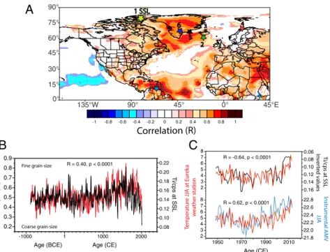
three-dimensional density data) and sediment accumulation rates indicate that the input of clastic sediment was very constant and uniform throughout the past 2,900 y (16). The varve chronology is based on multiple varve counts made on scanning electron microscope (SEM) images of 100 overlapping thin sections and is confirmed by several independent dating techniques (16). In modern times (past 120 y), radiometric dating shows excellent agreement with the varve chronology (16). Previous analysis showed that grain size is closely linked to summer temperature such that cool summers are characterized by sediments with a finer grain size (16). Furthermore, the finer grain-size fraction has a high level of titanium (Ti), and so Ti measured by high-resolution micro X-ray fluorescence (μ-XRF) scanning can be used as a proxy for summer temperature (Fig. 1 B and C). Results
Large-Scale Teleconnection. Changes in the geopotential height anomalies at 500 hPa across the North American High Arctic and Greenland are strongly correlated with Atlantic SSTs; this means that low pressure dominates the region during negative phases of the AMV when SSTs are below average (and vice versa). Low pressure in the High Arctic results in higher amounts of snow and a longer period of summer snowmelt; at SSL, this leads to higher levels of fine-grain sediments, containing a high level of Ti, being transported to the lake. These relationships are clearly shown in local weather records as well as in regional maps. The temperature record from Eureka, the nearest weather station to SSL (60 km northeast), shows good agreement with
both summer (June to August, JJA) AMV and Ti at SSL (r =
0.62, P < 0.0001, and r = −0.64, P < 0.0001, respectively), meaning cooler conditions occur during the negative phase of the AMV (AMV−), and this leads to higher Ti input in the lake (Fig. 1C). From May to August, higher snowfall is observed during times of cooler temperatures associated with lower
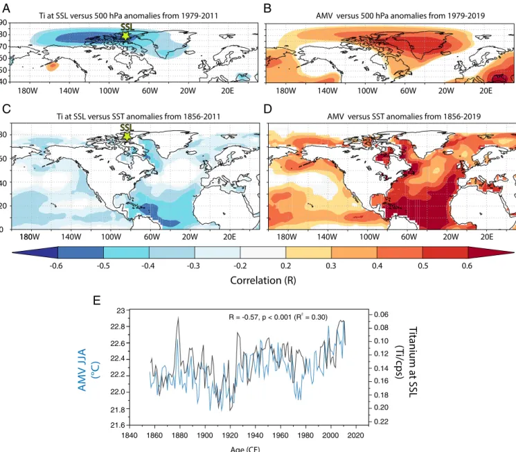
atmospheric pressure and increased cloud cover (21). This is coherent with the spatial correlation between 500 hPa geo-potential height and Ti at SSL which indicates a higher flux of Ti during times of lower atmospheric pressure (Fig. 2A). This pat-tern is essentially the same, but reversed in sign compared to the relationship between 500 hPa and AMV (Fig. 2B). Greater summer anticyclonic activity, linked with AMV+, leads to higher arctic temperatures and stronger sea ice loss, and less snowpack in arctic watersheds (21–27). Map correlations between instru-mental Atlantic SSTs (28) and Ti at SSL, and AMV versus SSTs show practically the same spatial patterns, but inversely corre-lated (Fig. 2 C and D). As sediments are mainly delivered to SSL by snowmelt (16, 20), anticyclonic conditions during AMV+ lead to decreased sedimentary input and correspondingly low levels of Ti (Fig. 2E). This is also revealed in spatial correlation where higher atmospheric pressure over most parts of North America in times of AMV+ promotes a depleted snow depth year-round (SI Appendix, Figs. S2 and S3).
Collectively, these relationships indicate that the SSL Ti re-cord can be reliably used to reconstruct AMV variability. Ti at SSL is strongly and negatively correlated to the instrumental AMV (r= −0.57, P < 0.0001, Fig. 2E) using the unsmoothed and unaltered version of the AMV (the detrended version also yielded a strong negative correlation; r= −0.46, P < 0.001, not shown). The maximum Ti concentration coincides with the coldest SSTs in the North Atlantic from∼1900–1925 CE, while lowest Ti values were found when SSTs were warmest, after ∼2005 CE.
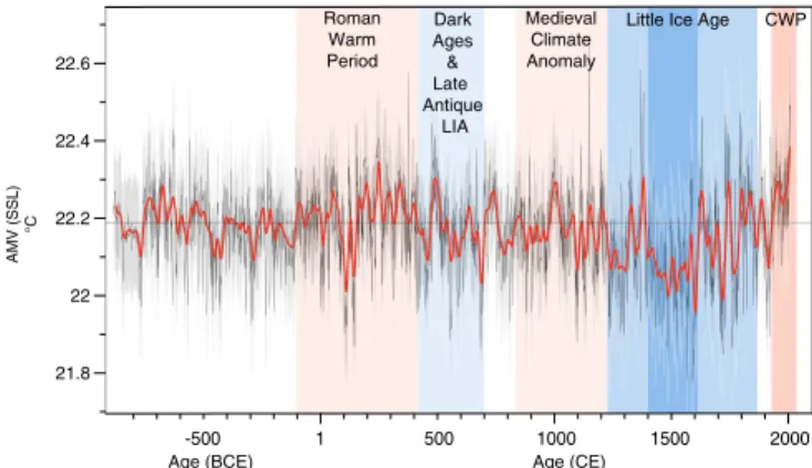
We use the strong correlation between the annual Ti record and the instrumental AMV to reconstruct past AMV (JJA) variability by regressing the Ti record onto the AMV (see Methods) to pro-duce a 2,900-y reconstruction of the AMV (hereafter AMVSSL) (Fig. 3). This shows multicentury and multidecadal variability in the AMV, with relatively warm conditions from ∼100 BCE to 1 SSL 6 4 2 5 3 Correlation (R) 7 0.06 0.08 0.10 0.12 0.14 0.16 R = -0.64, p < 0.0001 21.8 22.0 22.2 22.4 22.6 22.8 1950 1970 1990 2010 R = 0.62, p < 0.0001 2 3 4 5 6 7 8 2 3 4 5 6 7 8 Temperatur e JJA at E u re k a w e ather station T i/cps at SSL In ve rt ed values In strumental AMV JJA
A
C
90° 75° 60° 45° 30° 15° 0° 135°W 90° 45° 0° 45°E <16 µm (%) at SSL 0.2 0.3 0.4 0.5 0.6 0.7 0.8 0.9 T i/cps at SSL 0.08 0.10 0.12 0.14 0.16 0.18 0.20 0.22 -1000 1 1000 2000 Fine grain-size Coarse grain-sizeB
Age (CE) Age (CE) Age (BCE) R = 0.40, p < 0.0001Fig. 1. AMV during summer in the North Atlantic. (A) Spatial correlation between instrumental AMV and 2-m temperature from ERA-Interim (15) from 1979 to 2019. The numbering 1–7 corresponds to sites referred to in the text: SSL (1), Rapid-17–5P (2), A. islandica from bivalve shells (3), BWTs at Malagen (4), SIC in southeast Greenland (5), DYE-3 ice record (6), and G. bulloides abundance at Cariaco Basin (7). Map created using University of Maine Climate Reanalyzer,
https://climatereanalyzer.org/. (B) Annually fine grain size (%<16 μm) (16) compared to Ti at SSL (cps: counts per second) over the past 2,900 y. Data are
filtered by an 11-y Gaussian filter. (C, Upper) Comparison between SSL Ti (inverted values) and instrumental temperature (JJA, 3-y running mean) at Eureka weather station located 60 km northeast of SSL. (C, Lower) Same as Upper, but using the unsmoothed (and unaltered) instrumental AMV from Kaplan SST (17). Note that a turbidite dated to 1990 eroded 9 varves (16).
∼420 CE (the “Roman Warm Period”), followed by generally cooler conditions until the early 800s CE. This roughly corre-sponds to the“Dark Ages Cold Period” [∼410–775 CE (29)], al-though there were short multidecadal warm intervals within that period. The so-called“Late Antique Little Ice Age” (536–660 CE) was also a period of cooler SSTs (30). However, the longest and most persistent period of low SSTs was during the Little Ice Age (LIA:13th–18th centuries CE). Temperatures have steadily in-creased since the 15th century minimum; the rate and magnitude of warming over the last few centuries are unprecedented in the entire record, leading to the last decade which was the warmest of the past∼2,900 y.
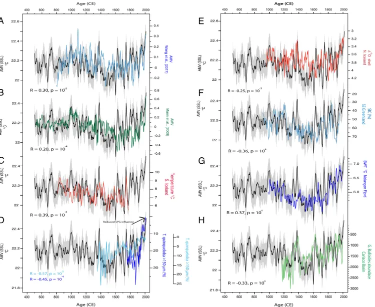
Our reconstructed AMVSSLis compared to other recent AMV reconstructions spanning the last 12–15 centuries in Fig. 4 A and B. In order to highlight the multidecadal variability of these re-cords, a 21-y Gaussian filter has been applied to both series. The
filtered time series denote periods of high covariability for the past 12 centuries suggesting that the AMVSSLprovides a robust long-term reconstruction, but additional confirmation is pro-vided by comparison with more direct paleoceanographic proxies (Fig. 4 C–H andSI Appendix, Tables S1 and S2).
High Temporal Resolution of Atlantic SST. To provide further evi-dence that the SSL record is linked to Atlantic SST, we compare the AMVSSLwith several highly resolved subdecadal marine re-cords from across the North Atlantic (Fig. 4 and SI Appendix, Tables S1 and S2). The Rapid-17–5P marine core, characterized
by extremely high temporal resolution (∼6 y), has been used to reconstruct thermocline temperature conditions south of Iceland using paired Mg/Ca-δ18O signals in the shells of the planktonic foraminifer Globorotalia inflata over the past∼1,200 y (31). As the first 600 m of the water column at this core site are dominated by
1840 1860 1880 1900 1920 1940 1960 1980 2000 2020 0.08 0.10 0.12 0.14 0.16 0.18 0.20 0.22
T
itanium at SSL
(T
i/cps)
21.6 21.8 22.0 22.2 22.4 22.6
AMV JJA
(°C
)
R = -0.57, p < 0.001 (R = 0.30) 2 Ti at SSL versus 500 hPa anomalies from 1979-2011A
B
Correlation (R)
180 140W 180W 100W 60W 20W 20E 180W 140W 100W 60W 20W 20E 20 40 60 80 0D
22.8 23 0.06 80 60 70 50 40 90 140W 180W 100W 60W 20W 20E 180W 140W 100W 60W 20W 20EAMV versus 500 hPa anomalies from 1979-2019
Ti at SSL versus SST anomalies from 1856-2011 AMV versus SST anomalies from 1856-2019
C
0.6 0.5 0.4 0.3 0.2 -0.2 -0.3 -0.4 -0.5 -0.6 Age (CE) SSL SSLE
Fig. 2. Ti variability at SSL and its relationship with instrumental AMV. (A) Map correlation between Ti variability and atmospheric pressure at 500 hPa from ERA-Interim (15) during summer (JJA) from 1979 to 2011. (B) Same as A but for the instrumental AMV (17) during summer (JJA) from 1979 to 2019. (C and D) Same as A and B but Ti at SSL (1856–2011) and instrumental AMV (1856–2019) correlated to SST anomalies from the Extended Reconstructed Sea Surface Temperature, version 5 (28). (E) Comparison between Ti at SSL (inverted values) and the instrumental summer (JJA) AMV over the instrumental period 1856–2011 (17). Yellow star (A and C) denotes the location of SSL record.
EARTH, ATMOS PHERIC, AND PLANETARY SCIENC ES
the northward flow of the North Atlantic Current, this area is well suited to record variability in North Atlantic SST (31). Comparing the records, there is a strong correlation between the AMVSSLand the Rapid-17–5P SST, suggesting that our record captures well the past SST variability in the vicinity of Iceland (Fig. 4C). Although the marine record Rapid-17–5P has an impressive sample reso-lution, its latest age is ∼1793 CE. New cores from this location have been collected and now extend the chronology to the present day (32). These new data show a drastic shift from sub-polar waters to warmer subtropical waters off southern Iceland during the 20th century (32). Turborotalita quinqueloba, a fora-minifer species that prefers cool and productive waters, has been declining at an accelerating pace during the past century and reached unprecedented low values in the last decade, in line with the unprecedented increase in the AMVSSL(Fig. 4D). This sug-gests a reduced influence of the subpolar gyre in recent decades compared to the past several millennia (32). Similarly, off the northern coast of Iceland, an annual record based onδ18O from shells of the long-lived marine bivalve Arctic islandica is also cor-related to AMVSSL(Fig. 4E). Spatial correlation analysis in in-strumental times (33) indicates that this δ18O-shell record correlates significantly with SST over much of Greenland, Iceland, and the Norwegian Sea.
A high-resolution (subdecadal) reconstruction of sea ice con-centration (SIC) for the coast of southeast (SE) Greenland highlights increased values from∼1400–1750 CE (34). This pe-riod coincides with the coldest SST anomalies in the North At-lantic (Fig. 4F) during the LIA. The overall covariability between the AMVSSLand the sea ice proxy is good at the resolution of the marine core. However, we note the existence of a lag of ∼45 y (sea ice leads) that is within the age uncertainties of the SIC record from Miettinen et al. (34), who reported a similar lag between the reconstructed SIC with reconstructed surface tem-perature. Finally, a comparison between the highly resolved bot-tom water temperature (BWT) at Malangen Fjord in Norway (Fig. 1) and our record also shows compelling covariability (Fig. 4G). This record, located∼2,800 km east of SSL, is a proxy for Atlantic heat flux at this latitude and the strength of the North Atlantic Current (37).
We also explored the AMVSSL with high-resolution records from tropical North Atlantic sites. A statistically significant negative correlation was found with the high-resolution (∼1.46 y) planktic foraminifer (Globigerina bulloides) abundance in the Cariaco Basin, Venezuela (Fig. 1). This anticorrelated relation-ship (Fig. 4H) is consistent with the spatial correlation between the G. bulloides abundance and historical SSTs showing the
highest negative anomaly in the North Atlantic (36). The G. bulloides abundance reflects cooler, more nutrient-rich waters and is associated with upwelling intensity and thus trade wind strength (36). This provides another line of evidence that our High-Arctic record is reliable as a proxy of multidecadal Atlantic SST and implies the existence of large-scale teleconnections between High-Arctic climate and basin-wide Atlantic variability. The significant correlations between our High-Arctic record and these widely distributed marine proxies, calculated from 10,000 bootstrap iterations using optimal block length (Methods andSI Appendix, Tables S1 and S2), point to a common climate signal linked to Atlantic SST variability.
The Past ∼3,000 y. A significant correlation was found between AMVSSLand the DYE-3δ18O record from southern Greenland (38), 2,000 km SE of SSL (Figs. 1A and 5A and SI Appendix, Tables S1 and S2). This ice core record is situated in that part of Greenland where the influence of North Atlantic maritime air masses is strong, and this is reflected in higher snow accumulation rates compared to the northern Greenland ice cores (39); it is thus ideally located to track past high-variability North Atlantic SST (40). The overall strong covariability between the AMVSSL and this ice core archive shows that southern Greenland and the Ca-nadian High Arctic shared a common climate pattern over the past∼3 millennia, driven by Atlantic SSTs (Fig. 5A).
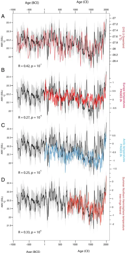
Reconstructed European temperature also show periods of high covariability and a significant correlation with the AMVSSLover the past 2,000 y (Fig. 5B andSI Appendix, Tables S1 and S2) (41). Observational evidence and climate models indicate that AMV+ has a strong influence on European summer temperature (43, 44). We note too that our record is strongly correlated with a summer pan-Arctic temperature reconstruction (41) (Fig. 5C) and with a Northern Hemisphere summer temperature reconstruction based on tree rings over the past ∼1,250 y (Fig. 5D) (42). This adds additional evidence that our High-Arctic lake record is recording large-scale climate teleconnections that can be linked to AMV. Discussion
The annually laminated sediments from SSL, Ellesmere Island, are strongly correlated with the AMV, due to atmospheric tel-econnections that affect summer temperatures and snow condi-tions in the Canadian High Arctic, and thus sediment flux to the lake. This is a robust and persistent relationship that can be seen in multiple terrestrial and marine proxies from the Canadian High Arctic, southern Greenland, Iceland and Norway, and the Cariaco Basin spanning the last 2 millennia. The SSL Ti record thus provides an excellent and unique 2,900-y proxy for AMV (Fig. 3).
Atlantic SST multidecadal variability has been a persistent feature of the climate system throughout the past∼3 millennia. Spectral analysis indicates statistically significant spectral peaks at∼11, 17, 32, 42, 83, and 112 y (SI Appendix, Fig. S4). The 11-y cycle closely matches the 11-y cycle found in the sunspot record. Without having a solid mechanism linking solar activity changes of 0.01% and climate variability, we do not link the 11-y cycle found in our record with solar forcing. However, we note that an 11-y cycle was detected in DYE-3 ice record and also the ∼20-and 43-y cycles (40). There was a strong 40–80 y periodicity during the LIA (13th–19th centuries CE), but this was only statistically significant in the interval during the 14th century and from∼1600 to present, a pattern compatible with another varve record in Iceland (45). The AMVSSLdepicts a long cooling trend from∼990 CE to 1400 CE, leading to the coldest period of the past 2,900 y, which occurred between∼1400–1605 CE. This is in line with in-creased sea ice off SE Greenland, lower δ18O values at DYE-3, and overall cooler SSTs around Iceland and Norway. Starting around the late 16th century, temperatures steadily rose, along with 21.8 22 22.2 22.4 22.6 AMV (SSL) °C 2000 1500 1 -500 500 1000 Age (CE) Age (BCE) Roman Warm Period Dark Ages & Late Antique LIA
Little Ice Age Medieval
Climate Anomaly
CWP
Fig. 3. Annual AMV changes over the past 2,900 y with a 30-y loess first-order low-pass filter (red). The gray horizontal line is the estimated average SST over the past 2,900 y (22.19°C). CWP denotes Current Warm Period. Shaded gray regions represent the 95% confidence intervals on the annual reconstructed AMVSSL, based on uncertainty estimates (Methods).
enhanced multidecadal variability as seen in the wavelet spectrum of AMVSSL(SI Appendix, Fig. S4).
The atmospheric pressure pattern in times of positive AMV (Fig. 2B) is reminiscent of the negative phase of the North At-lantic Oscillation (NAO). This is consistent with the negative correlation seen between the region (reconstructed AMV and Eureka weather station) and summer NAO (SI Appendix, Fig. S5). The DYE-3 ice record and temperature data from many weather stations in Greenland are also negatively correlated to NAO (46). The better covariability observed between AMVSSL
and DYE-3 δ18O in comparison with European temperature
might thus be attributable to the NAO influence on these two distant regions. The NAO involves a dipole pattern whereby the positive phase is characterized by warmth in Europe and cooler temperature in the western North Atlantic region, and vice versa. Of note is the strongest discrepancy between AMVSSLand Eu-ropean temperature occurring during the LIA, a feature not reflected in most of the other proxies (Fig. 4). A persistent positive state of NAO has been proposed to drive the periods of glacier
growth in Western Greenland and Baffin Island starting as early as ∼1200 CE (47), and this atmospheric pattern could explain the onset of the LIA earlier in the western North Atlantic than in Europe (48). Sea salt concentrations from GISP2 (49), a relative proxy for Icelandic Low (IL) and thereby NAO changes, highlight coherence with our record and reveal an abrupt deepening of the IL around 1400 CE, compatible with the strong declining trend in AMVSSL(SI Appendix, Fig. S6). Throughout the past 2,000 y, IL proxies indicate that periods of cooling, such as the Dark Ages Cold Period and the LIA (Roman Warm Period, Current Warm Period), correspond to a strengthening of the IL, and vice versa (50).
The dynamics between AMV and NAO is still not fully un-derstood (2). The impact of SSTs on the NAO has mainly been considered in the context of the NAO forced SST-tripole, the feedback of which is known to be weak (51). When considering the actual basin-scale SST associated with AMV, observational analysis and atmospheric model experiments show SST warming (cooling) leads to more frequent negative (positive) NAO (52–54). We note that the AMV relationship to the NAO is an
10 20 30 R = -0.57, p = 10 T. quinqueloba >150 μm (%) 0 10 20 5 15 25 T. quinqueloba >150 μm (%) R = -0.45, p = 10 22.4 22.2 AMV (SSL) °C 6 7 8 9 10 Temperature °C S. Iceland R = 0.39, p = 10-3 800 1000 1200 1400 1600 1800 2000 400 600 Age (CE) -5 -4 R = 0.30, p = 10-5 AMV Wang et al., (2017) 0.4 0.3 0.2 0.1 -0 -0.2 800 1000 1200 1400 1600 1800 2000 400 600 Age (CE) 6.0 6.5 7.0 BWT °C Malangen Fjord 500 1000 1500 2000 2500 3000 G. Bulloides abundac e Ca riac o Basin R = 0.37, p = 10-5 R = -0.25, p = 10-3 3 3.2 3.4 3.6 3.8 4 4.2 δ O shell N. Iceland 18 R = 0.20, p = 10 0.8 0.6 0.4 0.2 0 -0.2 -0.4 -0.6 AMV Mann et al., (2009) 800 1000 1200 1400 1600 1800 2000 400 600 Age (CE) Age (CE) -4 R = -0.36, p = 10-4 R = -0.33, p = 10-5 20 30 40 50 60 70 SIC (%) SE Gr eenland 800 1000 1200 1400 1600 1800 2000 400 600 Age (CE) 22 22.4 22.2 AMV (SSL) °C 22 22.4 22.2 AMV (SSL) °C 22 22.4 22.2 AMV (SSL) °C 22 22.4 22.2 AMV (SSL) °C 22 22.4 22.2 AMV (SSL) °C 22 22.4 22.2 AMV (SSL) °C 22 22.6 21.8 22.4 22.2 AMV (SSL) °C 22 22.6 21.8
A
C
B
E
F
G
H
D
Fig. 4. SSL record and its relationship with subdecadal Atlantic SST. (A) AMV based on the Ti record from SSL (AMVSSL) compared to reconstructed AMV (12).
(B to H) Same as A but AMVSSLcompared to AMV from Mann et al. (B) (13), ocean temperature south of Iceland from core Rapid-17–5P (C) (31), T.
quin-queloba (light blue) from core EN539-MC14-A and T. quinquin-queloba (dark blue) from core MC16-A (D) (32), theδ18O from shells of the long-lived marine bivalve
A. islandica (E) (33), the SIC off SE Greenland (F) (34), the BWT at Malangen Fjord (G) (35); and G. bulloides abundance from Cariaco Basin (H) (36). In D, SPG stands for subpolar gyre. Shaded gray regions represent the 95% confidence intervals on the reconstructed AMVSSL, based on uncertainty estimates
(Methods). EARTH, ATMOS PHERIC, AND PLANETARY SCIENC ES
emerging area of research, and currently, inconsistencies in dif-ferent reconstructions of the NAO (and AMV) before the in-strumental period make it difficult to come to firm conclusions (2). However, our record provides support for a link between
AMV and IL variability over the past 2,900 y, suggesting a pos-sible link between AMV and long-term NAO in the past (SI Appendix, Fig. S6). In summary, differences in the time series may be related to changes in the NAO, but the overall strong
−1000 −500 1 500 1000 2000 Europe temperatures PAGES 2k 1 0.5 0 -0.5 0.5 0 -0.5 -1 -1.5 Arctic temperatures PAGES 2k −1000 −500 1 500 1000 1500 2000 1500 Age (CE) Age (BCE) Age (CE) Age (BCE) R = 0.27, p = 10 R = 0.42, p = 10 R = 0.25, p = 10 -7 -6 -5 d n al n e er G 3-E Y D O δ -27 -27.2 -27.4 -27.8 -28 -28.2 -28.4 8 1 R = 0.33, p = 10-6 3 2 1 0 -1 -2
Summer Northern Hemnisphere temperature
tree-rings Ntrend 22.4 22.3 22.2 22.1 AMV (SSL) °C 22 21.9 22.4 22.3 22.2 22.1 AMV (SSL) °C 22 22.4 22.3 22.2 22.1 AMV (SSL) °C 22 22.4 22.3 22.2 22.1 AMV (SSL) °C 22 -27.6
A
B
C
D
Fig. 5. Northern Hemisphere high-resolution proxy records spanning the past∼3 millennia. (A) Comparison between DYE-3 Greenland δ18O record (38) and
the AMVSSL(this study). (B and C) same as A, but AMVSSLis compared to European (B) and Arctic (C) temperature reconstructions over the past 2,000 y from
PAGES 2K (41). (D) AMVSSLis compared with reconstructed Northern Hemisphere temperature based on tree rings (42). All time series filtered by a 21-y
coherence between them is associated with the background state of the AMV.
Within the measurement period, the period post 2005 coin-cides with unprecedented anticyclonic conditions in the region, which have been linked to warmer Atlantic SSTs, negative NAO, and increased Greenland Blocking Index (22, 25, 55, 56). These sustained higher-pressure atmospheric anomalies have led to record melting of Arctic Canadian ice caps and also the Greenland ice sheet in the past decade and are associated with decreased snow depth during summer which acts to decrease albedo and further increase warming. Thus, the dynamics be-tween NAO and AMV is a topic of great interest for future melting of arctic ice caps, especially the Greenland ice sheet (25). Importantly, all of the records shown here denote that the warmest interval occurred during the past decade, which also coincides with the retreat of subpolar conditions south of Iceland (Fig. 4D). On a decadal-scale basis, results suggest that the re-cent Atlantic warming is unparalleled in the context of the last ∼2,900 y.
Methods
Geochemicalμ-XRF. μ-XRF data were acquired using an ITRAX core scanner available at Institut National de la Recherche Scientifique–Eau Terre Envi-ronnement in Québec City. High-resolution geochemical variations (57) were measured using a molybdenum tube. The data acquisition was performed at 100μm resolution with an exposure time of 15 s. Voltage and current were 30 kV and 30 mA with counts per second ranging from 26,000–34,000. All elements were normalized by the total of counts for each spectrum. To obtain annually resolvedμ-XRF Ti data, we used the thickness of each layer calculated in thin sections and averaged the values over the corresponding depth year. A code was written to compute annualμ-XRF in R (58). Annual Grain Size. One hundred overlapping thin sections were made to span the annually laminated section of the SSL varve record. Thin sections were digitized using a flatbed scanner at 2,400 dots per inch (1 pixel= 10.6 μm). Annual grain-size data were extracted using the image analysis technique that uses high-resolution images (1,024× 768 pixels, 1 pixel = 1 μm) collected from thin sections at the SEM in backscattered electron (BSE) mode (Zeiss Evo 50 SEM). Approximately eight thousand 8-bit gray-scale SEM images in BSE mode were acquired to collect grain-size data for the past 2,900 y (16). Instrumental AMV and Meteorological Data. The instrumental AMV has been extracted from National Oceanic and Atmospheric Administration (NOAA) (17). The instrumental AMV used in this study is from the Kaplan SST V2. The data are monthly average SST interpolated to a 5× 5 grid over the North Atlantic, 0°–70°N (59). Correlation maps were prepared using the Climate Explorer tool that is managed by the Royal Netherlands Meteorological In-stitute (60). Atmospheric pressure data are from ERA-Interim reanalysis (15).
Meteorological data from Eureka weather station (Ellesmere Island, Canada) were extracted from the historical climate data from the Govern-ment of Canada (61).
AMV Reconstruction. To estimate past summer SST in the North Atlantic (0°–70°N) we use ordinary least squares regression between the Ti data at SSL and instrumental AMV during summer (JJA). The uncertainty in the re-construction (gray-shaded values in Figs. 3–5) was assessed using 95% bootstrap confidence intervals from 2,000 bootstrap samples (62, 63). Bootstrap Confidence Intervals for Correlations. For archives that are not annually resolved, data were first resampled at the lowest time resolution of the corresponding archive using linear interpolation (SI Appendix, Table S1). Then, correlation analysis between reconstructed AMVSSLand several North
Atlantic proxy records was performed. r is the Pearson’s correlation coeffi-cient, and P is the probability that two uncorrelated datasets would exhibit a stronger correlation. The percentile confidence intervals at 95% were cal-culated from 10,000 nonparametric stationary bootstrap iterations (64) us-ing optimal block length followus-ing Patton et al. (65). This analysis was done using R package“tsboot” (66).SI Appendix, Table S1shows the correlation results for the unfiltered data with the 95% confidence intervals.
The annual time series (12, 13, 33, 36, 41, 42) were filtered by a 21-y Gaussian smoothing function (Figs. 4 and 5). For the subdecadal records, i.e., the temperature (31) and the T. quinqueloba (32) records from southern Iceland, the SIC SE Greenland (34) and the DYE-3 ice record (38) were filtered by a 3-point Gaussian function (Fig. 4). The coefficient correlations and P values found in Figs. 4 and 5 are the mean Pearson’s correlation and the mean P values for the filtered data based on the 10,000 nonparametric stationary bootstrap iterations with consideration for autocorrelation (67).
SI Appendix, Table S2shows the same analysis but using a 21-y centered
running mean on the annual series and 3-point centered running mean for subdecadal records, which yielded higher correlation coefficient.
Wavelet and Spectral Analysis. Wavelet analysis was carried out with the R package“biwavelet” (58, 68), and spectral analysis was performed using the software REDFIT (69) (SI Appendix, Fig. S4).
Data Availability. The data are available from the World Data Center for Paleoclimatology (70).
ACKNOWLEDGMENTS. We thank the Polar Continental Shelf Program, Canada Natural Resources, for help with field preparations and logistic inputs. We are grateful to Natural Sciences and Engineering Research Council of Canada discovery and northern supplement grants (Grants RGPIN-2014-05810 and RGPNS-2014-305427 [to P.F.]). We also acknowledge support from NSF Grants OPP-1744515 and PLR-1417667 to the University of Massachusetts. M.B.A. acknowledges support from NSF Grant 1215661. We thank Rong Zhang for helpful comments. F.L. is grateful to the Fonds de Recherche Nature et Technologies du Québec and the Weston Garfield Foundation for external grants. We are grateful to two anonymous referees whose comments helped improve the final manuscript.
1. R. Sutton et al., Atlantic multidecadal variability and the UK ACSIS program. Bull. Am. Meteorol. Soc. 99, 415–425 (2018).
2. R. Zhang et al., A review of the role of the Atlantic meridional overturning circulation in Atlantic multidecadal variability and associated climate impacts. Rev. Geophys. 57, 316–375 (2019).
3. R. T. Sutton, D. L. Hodson, Atlantic Ocean forcing of North American and European summer climate. Science 309, 115–118 (2005).
4. C. K. Folland, T. N. Palmer, D. E. Parker, Sahel rainfall and worldwide sea tempera-tures, 1901–85. Nature 320, 602–607 (1986).
5. A. Giannini, R. Saravanan, P. Chang, Oceanic forcing of Sahel rainfall on interannual to interdecadal time scales. Science 302, 1027–1030 (2003).
6. J. Lu, T. L. Delworth, Oceanic forcing of the late 20th century Sahel drought. Geophys. Res. Lett. 32, L22706 (2005).
7. R. Zhang, T. L. Delworth, Impact of Atlantic multidecadal oscillations on India/Sahel rainfall and Atlantic hurricanes. Geophys. Res. Lett. 33, L17712 (2006).
8. M. Ting, Y. Kushnir, R. Seager, C. Li, Robust features of Atlantic multi‐decadal vari-ability and its climate impacts. Geophys. Res. Lett. 38, L17705 (2011).
9. R. Seager et al., Tropical oceanic causes of interannual to multidecadal precipitation variability in southeast South America over the past century. J. Clim. 23, 5517–5539 (2010).
10. S. B. Goldenberg, C. W. Landsea, A. M. Mestas-Nuñez, W. M. Gray, The recent increase in Atlantic hurricane activity: Causes and implications. Science 293, 474–479 (2001). 11. R. T. Sutton, D. L. Hodson, Climate response to basin-scale warming and cooling of the
North Atlantic Ocean. J. Clim. 20, 891–907 (2007).
12. J. Wang et al., Internal and external forcing of multidecadal Atlantic climate vari-ability over the past 1,200 years. Nat. Geosci. 10, 512–517 (2017).
13. M. E. Mann et al., Global-scale signatures and dynamical origins of the Little Ice Age and Medieval Climate Anomaly. Science 326, 1256–1260 (2009).
14. S. T. Gray, L. J. Graumlich, J. L. Betancourt, G. T. Pederson, A tree‐ring based recon-struction of the Atlantic multidecadal oscillation since 1567 AD. Geophys. Res. Lett. 31, L12205 (2004).
15. D. Dee et al., The ERA‐Interim reanalysis: Configuration and performance of the data assimilation system. Q. J. R. Meteorol. Soc. 137, 553–597 (2011).
16. F. Lapointe et al., Chronology and sedimentology of a new 2.9 ka annually laminated record from South Sawtooth Lake, Ellesmere Island. Quat. Sci. Rev. 222, 105875 (2019).
17. D. B. Enfield, A. M. Mestas-Nunez, P. J. Trimble, The Atlantic multidecadal oscillation and its relation to rainfall and river flows in the continental U. S. Geophys. Res. Lett. 28, 2077–2080 (2001).
18. P. Francus, R. S. Bradley, M. B. Abbott, W. Patridge, F. Keimig, Paleoclimate studies of minerogenic sediments using annually resolved textural parameters. Geophys. Res. Lett. 29, 59–1–59–4 (2002).
19. J. England et al., The Innuitian ice sheet: Configuration, dynamics and chronology. Quat. Sci. Rev. 25, 689–703 (2006).
20. P. Francus et al., Limnological and sedimentary processes at Sawtooth Lake, Canadian High Arctic, and their influence on varve formation. J. Paleolimnol. 40, 963–985 (2008). 21. E. M. Knudsen, Y. J. Orsolini, T. Furevik, K. I. Hodges, Observed anomalous atmo-spheric patterns in summers of unusual Arctic sea ice melt. J. Geophys. Res. D At-mospheres 120, 2595–2611 (2015).
22. P. Bezeau, M. Sharp, G. Gascon, Variability in summer anticyclonic circulation over the Canadian Arctic Archipelago and west Greenland in the late 20th/early 21st centuries and its effect on glacier mass balance. Int. J. Climatol. 35, 540–557 (2015).
EARTH, ATMOS PHERIC, AND PLANETARY SCIENC ES
23. H. Wernli, L. Papritz, Role of polar anticyclones and mid-latitude cyclones for Arctic summertime sea-ice melting. Nat. Geosci. 11, 108–113 (2018).
24. H. Tokinaga, S.-P. Xie, H. Mukougawa, Early 20th-century Arctic warming intensified by Pacific and Atlantic multidecadal variability. Proc. Natl. Acad. Sci. U.S.A. 114, 6227–6232 (2017).
25. L. Hahn, C. Ummenhofer, Y. O. Kwon, North Atlantic natural variability modulates emergence of widespread Greenland melt in a warming climate. Geophys. Res. Lett. 45, 9171–9178 (2018).
26. A. Rinke et al., Arctic summer sea ice melt and related atmospheric conditions in coupled regional climate model simulations and observations. J. Geophys. Res. D Atmos. 124, 6027–6039 (2019).
27. J. A. Screen, I. Simmonds, K. Keay, Dramatic interannual changes of perennial Arctic sea ice linked to abnormal summer storm activity. J. Geophys. Res. D Atmos. 116, D15105 (2011).
28. B. Huang et al., Extended reconstructed sea surface temperature, version 5 (ERSSTv5): Upgrades, validations, and intercomparisons. J. Clim. 30, 8179–8205 (2017). 29. S. Helama, P. D. Jones, K. R. Briffa, Dark Ages Cold Period: A literature review and
directions for future research. Holocene 27, 1600–1606 (2017).
30. U. Büntgen et al., Cooling and societal change during the Late Antique Little Ice Age from 536 to around 660 AD. Nat. Geosci. 9, 231–236 (2016).
31. P. Moffa-Sánchez, A. Born, I. R. Hall, D. J. Thornalley, S. Barker, Solar forcing of North Atlantic surface temperature and salinity over the past millennium. Nat. Geosci. 7, 275–278 (2014).
32. P. T. Spooner et al., Exceptional 20th century ocean circulation in the northeast At-lantic. Geophys.Res. Lett. 47, e2020GL087577 (2020).
33. D. J. Reynolds et al., Annually resolved North Atlantic marine climate over the last millennium. Nat. Commun. 7, 13502 (2016).
34. A. Miettinen, D. V. Divine, K. Husum, N. Koç, A. Jennings, Exceptional ocean surface conditions on the SE Greenland shelf during the medieval climate anomaly. Paleo-ceanography 30, 1657–1674 (2015).
35. L. K. Cunningham et al., Reconstructions of surface ocean conditions from the northeast Atlantic and Nordic seas during the last millennium. Holocene 23, 921–935 (2013).
36. D. E. Black et al., Eight centuries of North Atlantic Ocean atmosphere variability. Science 286, 1709–1713 (1999).
37. M. Hald, G. Salomonsen, K. Husum, L. Wilson, A 2000 year record of Atlantic water temperature variability from the Malangen Fjord, northeastern North Atlantic. Ho-locene 21, 1049–1059 (2011).
38. B. M. Vinther et al., Holocene thinning of the Greenland ice sheet. Nature 461, 385–388 (2009).
39. D. Dahl-Jensen et al., Past temperatures directly from the Greenland ice sheet. Science 282, 268–271 (1998).
40. P. Chylek et al., Greenland ice core evidence for spatial and temporal variability of the Atlantic multidecadal oscillation. Geophys. Res. Lett. 39, L09705 (2012).
41. PAGES 2k Consortium, Continental-scale temperature variability during the past two millennia. Nat. Geosci. 6, 339–346 (2013).
42. R. Wilson et al., Last millennium Northern Hemisphere summer temperatures from tree rings: Part I: The long term context. Quat. Sci. Rev. 134, 1–18 (2016). 43. J. R. Knight, C. K. Folland, A. A. Scaife, Climate impacts of the Atlantic multidecadal
oscillation. Geophys. Res. Lett. 33, L17706 (2006).
44. R. T. Sutton, B. Dong, Atlantic Ocean influence on a shift in European climate in the 1990s. Nat. Geosci. 5, 788–792 (2012).
45. K. B. Olafsdottir, Á. Geirsdóttir, G. H. Miller, D. J. Larsen, Evolution of NAO and AMO strength and cyclicity derived from a 3-ka varve-thickness record from Iceland. Quat. Sci. Rev. 69, 142–154 (2013).
46. B. M. Vinther et al., Climatic signals in multiple highly resolved stable isotope records from Greenland. Quat. Sci. Rev. 29, 522–538 (2010).
47. V. Jomelli et al.; ASTER Team, Paradoxical cold conditions during the medieval climate anomaly in the Western Arctic. Sci. Rep. 6, 32984 (2016).
48. N. E. Young, A. D. Schweinsberg, J. P. Briner, J. M. Schaefer, Glacier maxima in Baffin Bay during the Medieval Warm Period coeval with Norse settlement. Sci. Adv. 1, e1500806 (2015).
49. P. A. Mayewski et al., Major features and forcing of high‐latitude Northern Hemi-sphere atmospheric circulation using a 110,000‐year‐long glaciochemical series. J. Geophys. Res. Oceans 102, 26345–26366 (1997).
50. J. D. Auger et al., 2000 years of North Atlantic-Arctic climate. Quat. Sci. Rev. 216, 1–17 (2019).
51. Y. Kushnir et al., Atmospheric GCM response to extratropical SST anomalies: Synthesis and evaluation. J. Clim. 15, 2233–2256 (2002).
52. N.-E. Omrani, N. S. Keenlyside, J. Bader, E. Manzini, Stratosphere key for wintertime atmospheric response to warm Atlantic decadal conditions. Clim. Dyn. 42, 649–663 (2014).
53. Y. Peings, G. Magnusdottir, Forcing of the wintertime atmospheric circulation by the multidecadal fluctuations of the North Atlantic Ocean. Environ. Res. Lett. 9, 034018 (2014).
54. N. Keenlyside, N.-E. Omrani, Has a warm North Atlantic contributed to recent Euro-pean cold winters? Environ. Res. Lett. 9, 061001 (2014).
55. M. Tedesco et al., Arctic cut-off high drives the poleward shift of a new Greenland melting record. Nat. Commun. 7, 11723 (2016).
56. M. Tedesco, X. Fettweis, Unprecedented atmospheric conditions (1948–2019) drive the 2019 exceptional melting season over the Greenland ice sheet. Cryosphere 14, 1209–1223 (2020).
57. I. W. Croudace, A. Rindby, R. G. Rothwell, ITRAX: Description and evaluation of a new multi-function X-ray core scanner. Spec. Publ. Geol. Soc. Lond. 267, 51–63 (2006). 58. R Core Team, R: A Language and Environment for Statistical Computing, Version
3.5.1, (R Foundation for Statistical Computing, Vienna, 2017).
59. NOAA Physical Sciences Laboratory, Climate timeseries: AMO (Atlantic Multidecadal Oscillation) Index. https://psl.noaa.gov/data/timeseries/AMO/. Accessed 29 September 2020.
60. G. J. Van Oldenborgh, G. Burgers, Searching for decadal variations in ENSO precipi-tation teleconnections. Geophys. Res. Lett. 32, L15701 (2005).
61. Government of Canada, Monthly data report for 1948. https://climat.meteo.gc.ca/ climate_data/monthly_data_e.html?hlyRange=1953-01-01%7C2016-02-25&dlyRange=1947-05-01%7C2016-02-24&mlyRange=1947-01-01%7C2016-02-01&StationID=1750&Prov=NU &urlExtension=_e.html&searchType=stnName&optLimit=yearRange&StartYear=1840 &EndYear=2019&selRowPerPage=25&Line=0&searchMethod=contains&txtStationName= Eureka&timeframe=3&Month=10&Day=8&Year=1948#. Accessed 29 September 2020. 62. J. Fox, Nonparametric Simple Regression: Smoothing Scatterplots, (Sage, 2000). 63. J. Fox, S. Weisberg, An R Companion to Applied Regression, (Sage publications, 2018). 64. M. Mudelsee, Climate Time Series Analysis: Classical Statistical and Bootstrap
Meth-ods: Atmospheric and Oceanographic Sciences Library, (2010), Vol. 42.
65. A. Patton, D. N. Politis, H. White, Correction to“Automatic block-length selection for the dependent bootstrap” by D. Politis and H. White. Econom. Rev. 28, 372–375 (2009).
66. A. Canty, M. B. Ripley, Package“boot.” Version 1.3-25. https://cran.r-project.org/web/ packages/boot/boot.pdf. Accessed 22 May 2020.
67. M. Mudelsee, Trend analysis of climate time series: A review of methods. Earth Sci. Rev. 190, 310–322 (2019).
68. T. C. Gouhier, A. Grinsted, V. Simko, R package“biwavelet”: Conduct univariate and bivariate wavelet analyses. Version 0.20.15. https://github.com/tgouhier/biwavelet. Accessed 9 April 2020.
69. M. Schulz, M. Mudelsee, REDFIT: Estimating red-noise spectra directly from unevenly spaced paleoclimatic time series. Comput. Geosci. 28, 421–426 (2002).
70. F. Lapointe, R. S. Bradley, P. Francus, Sawtooth Lake, Ellesmere Island 2,900 year annual titanium data and AMVI reconstruction. National Oceanic and Atmospheric Administration. https://www.ncdc.noaa.gov/paleo/study/31353. Deposited 25 September 2020.