2004 — Modelling of calibration steam flowmeter test bench

THESIS SUBMITTED TO

ÉCOLE DE TECHNOLOGIE SUPÉRIEURE

IN FULFILLMENT OF THE REQUIREMENTS FOR THE DEGREE OF MASTER IN ENGINEERING MECHANICS

M.Eng

BY

NAM TUAN PHUONG LE

MODELLING OF CALIBRATION STEAM FLOWMETER TEST BENCH

MONTREAL, JANUARY 15, 2004

THIS THESIS IS EV ALUATED BY THE JURY COMPOSED OF :

M. Christian Masson, president of jury

Department of Mechanical Engineering, École de technologie supérieure

M. Louis Lamarche, director of thesis

Department ofMechanical Engineering, École de technologie supérieure

M. Stanislaw Kajl, co-director ofthesis

Department of Mechanical Engineering, École de technologie supérieure

M. Gérald Bénard, engineer Preston Phipps Inc

THIS THESIS WAS PRESENTED IN FRONT OF JURY AND PUBLIC ON DECEMBER 17, 2003

Nam Tuan Phuong Le SOMMAIRE

Ce présent projet développe des méthodes de simulation pour le banc d'essai utilisé pour calibrer le débitmètre de vapeur en utilisant la vapeur comme le fluide de travail. Ce banc d'essai est équipé avec un condenseur de vapeur. Le condensât mesuré dans une période de temps donnée en régime permanent est employé pour calibrer le débitmètre. Deux modèles mathématiques sont développés pour étudier le transfert de chaleur dans le condenseur. Il s'agit d'un échangeur thermique de type tube et calandre. Basé sur la théorie du réseau de neurones, le premier modèle est pour prédire la température, la pression et le débit du vapeur et la hauteur du condensât. Les paramètres d'entrée pour ce modèle sont la position d'ouverture des valves de contrôle et la température d'entrée de l'eau de refroidissement.

Le second modèle (modèle physique) est basé sur la conservation de la masse et de 1 'énergie. Pour augmenter la précision, le condenseur est divisé en volumes de contrôle auxquels l'équilibre de la masse et de l'énergie sont appliqué. Le modèle décrit la réponse du système en différentes variables, y compris le niveau du condensât et la pression de la vapeur dans l'échangeur thermique. Les valeurs d'entrée de ce modèle sont la position d'ouverture des valves, le débit et la température d'entrée de l'eau de refroidissement.

Ces deux modèles donnent de bons résultats comparés aux données expérimentales. Cependant, le modèle physique est préféré grâce à sa capacité de construire des relations entre des paramètres physiques du problème. Il est suggéré que dans le futur travail, ce modèle soit employé pour modéliser un système de contrôle à multivariables, qui est pour la régulation du niveau du condensât et la pression de la vapeur.

MODELLING OF CALIBRATION STEAM FLOWMETER TEST BENCH Nam Tuan Phuong Le

ABSTRACT

The present project develops simulation methods for the test hench that serves to calibrate the steam flowmeters by using steam as working fluid. The test hench contains a condenser, the purpose of which is to condense the steam. By maintaining a steady-state regime, the weight of condensate measured during a given period of the time is used to calibrate the steam flowmeter.

Two mathematical models are developed in this project for the heat transfer process within the condenser, which is a shell-and-tube heat exchanger. The first model is based on neural network theory for predicting steam temperature, pressure, flow and the height of condensate. The input parameters to this model include the opened-closed position of the control valves and the inlet temperature of the cooling water.

The second model (physical model) is based on the mass and energy conservation principles. For increasing the accuracy, the condenser is divided into control volumes to which the mass and energy balances are applied. The model describes the dynamic response of the system at different locations including the condensate level and the steam pressure within the heat exchanger. The input values are the opened-closed position of the valves, the flow rate and inlet temperature of cooling water.

Both of these models give satisfactory results compared with experimental data. However, the physical model is preferred by its capability of explaining the relationships between parameters. It is suggested for a future work that physical model is applied to a multivariable control system for the regulation of the level of condensate and the steam pressure.

thermique au Centre de technologie thermique - École de technologie supérieure à Montréal. Le modèle sert à la calibration d'un débitmètre de vapeur. La connaissance du comportement dynamique de cet échangeur est important pour cmmaître la réponse du système au changement de débit, de température ou de pression. Ces informations sont vraiment nécessaires pour concevoir des contrôleurs d'un tel système.

Ce travail va présenter deux approches pour la modélisation de cet échangeur thermique. Le rapport comprend cinq chapitres.

Le premier chapitre fait une revue de la littérature portant sur la modélisation et simulation d'échangeur thermique de type 'shell et tube' et de l'application du réseau de neurones dans la modélisation et la simulation.

Le deuxième chapitre décrit le système de calibration du débitmètre de vapeur et de l'opération du système de calibration suivant : la vapeur est alimentée par source de vapeur extérieure au système de condensateur à la pression 862 kPa. Le débit de vapeur est commandé par une vanne de contrôle. La vapeur après la vam1e de contrôle est dirigée vers l'échangeur du type "shell et tube" et suivant un échange thermique avec l'eau froide à l'intérieur des tuyaux. L'eau qui se forme pendant la condensation est stockée en bas de l'échangeur et est ensuite amenée dans un réservoir et mesurée pour calibrer le débitmètre. La construction de l'échangeur thermique est présentée avec des dimensions géométriques.

La modélisation de notre échangeur thermique a été réalisée en utilisant deux approches différentes: une est basée sur les réseaux de neurones et l'autre sur le principe de conservation de matière et d'énergie.

lV

Le troisième chapitre décrit le développement du modèle en utilisant le réseau de neurones. Ce modèle est capable de prédire le débit, la température et la pression de vapeur ainsi que le niveau d'eau condensée dans l'échangeur thermique. Cette nouvelle approche est largement utilisée dans plusieurs domaines : en finance, en ingénierie ... et elle est maintenant utilisée dans notre travail. La procédure de modélisation passe par les étapes suivantes :

1. Détermination des inputs & outputs 2. Choix des données expérimentales 3. Division des données

4. Normalisation de données

5. Détermination de l'architecture de réseau 6. Application

Pendant la première étape, les paramètres d'entrée et de sortie du réseau de neurones doivent être déterminés.

Les entrées sont :

-Les positions d'ouverture des trois valves VR2-1V; VRl-lV; VRl-lC -La température de l'eau refroidissant CTl-lE

Les sorties sont :

-La pression, la température, le débit de vapeur. -Le niveau de condensât dans l'échangeur thermique.

Les données expérimentales mesurées au laboratoire sont utilisés pour déterminer les entrées et smiies afin de former le réseau de neurones. Les données expérimentales

contiennent toujours du bruit. Par conséquent, les données stables sont choisies pour l'entraînement (training) le réseau de neurones et les données stables sont divisées en sous-groupes.

Selon la pratique courante, les données disponibles sont divisées en deux sous-groupes : un groupe pour l'entraînement (training) et un autre groupe indépendant pour la validation. Mais les données stables (après le filtrage du bruit) sont divisées en trois sous-groupes : un pour 1' entraînement, un autre pour la validation et le troisième pour le test. Le sous-groupe pour le test est utilisé pour vérifier la performance du modèle à différentes étapes du processus d'apprentissage. Les erreurs détectées ici ne sont pas utilisées pendant 1' entraînement mais plutôt pour comparer la performance de différents modèles.

Les données sont divisées en trois sous-groupes mentionnés plus haut de la façon suivante:

1. Un quart est utilisé pour la validation. 2. Un autre quart pour le test.

3. La moitié qui reste est utilisée pour le traitement.

Après la division des données, les inputs et outputs sont normalisées à l'aide des fonctions premnmx, postmnmx disponibles dans Matlab avec les critères Max et Min de telle façon qu'elles se trouvent dans l'intervalle [-1;1].

Dans cinquième étape, il faut déterminer l'architecture du réseau de neurones. C'est une tâche très importante dont le but est de déterminer le nombre de couches dans le réseau de neurones, le nombre de neurones dans chaque couche, la fonction de transfert et 1' algorithme mathématique.

Vl

Pour ce projet, un réseau comportant quatre couches avec une couche pour l'entrée de données (inputs), deux couches cachées et une couche pour la sortie de données (outputs). La première couche cachée contient 16 nœuds et la deuxième en contient 40, donc le rapport des nœuds de ces deux couches cachées est 1 : 2.5. Ce rapport a été obtenu par la méthode "trial and error". Le nombre de nœuds dans la couche outputs est égale au nombre de sorties (4) et le nombre de nœuds dans la couche d'entrée de données (inputs) est aussi égale au nombre des entrées (4). La fonction de transfert: la fonction log-sigmoid pour toutes les couches cachées et la fonction purelin pour la couche de sortie

L'algorithme 'back-propagation' qui utilise la méthode de SCG (scaled conjugate gradient) développée par Mo 11er [ 11] est choisi pour calculer des vecteurs de gradient pour mettre à jour les degrés de liberté.

1. Les degrés de liberté sont initialisés à zéro. 2. La taille d'Epoch (mode Batch) est égale à 75. 3. Le taux d'apprentissage est égal à 0. 5

4. Critère d'arrêt : critère de 'cross-validation' est utilisé.

Finalement, après l'arrêt de processus d'apprentissage, un ensemble de données indépendantes sont utilisés pour valider le modèle comme c'est montré dans le rapport à la page 25 et 26.

Dans la section " Normalisation de données ", les données sont normalisées. De cette façon, pour valider le modèle avec un ensemble de données indépendantes, il faut vérifier que les inputs se trouvent dans 1' intervalle [ -1; 1] avec les critères Max et Min définis plus haut. Cela signifie que les valeurs maximales et minimales de l'ensemble des données indépendantes ne dépassent pas les valeurs maximales et minimales des données d'entraînement.

Maintenant la capacité générale du réseau de neurones est améliorée et les intervalles d'opération suivante du modèle:

- Pour la valve de vapeur : 5% - 100 % (VR2-l V)

-Pour la valve de l'eau condensée: 5.2%-6.5% (VRl-lC)

-Pour la température d'entrée de l'eau froide: 119°F- 131 °F (CTl-lE)

Dans le quatrième chapitre, un modèle physique est développé pour le même système de condensateur de vapeur précédemment décrit. Cette approche est basée sur la conservation de masse et d'énergie. Le modèle physique a même l'objectif comme le modèle de réseau de neurones, qui est de prédire des quantités de sorties (la pression de vapeur et le niveau d'eau condensée) en fonction des entrées. Les entrées du modèle physique comprend les paramètres : La position de l'ouverture de valve, la température d'entrée de l'eau froide et le débit de l'eau froide. De plus, le modèle physique décrit dynamiquement le système d'une condition initiale dans tout régime transitoire jusqu'à ce que la condition du régime permanent soit atteinte, alors que le modèle de réseau de neurones traite juste des états d'état d'équilibre.

L'échangeur thermique est divisé en trois volumes de contrôle (V.C.) où les deux premiers V.C. pour le condensât se trouve en bas et le troisième V.C. pour la vapeur se trouve en haut du shell. Pour le faire, les hypothèses suivantes sont considérées :

-La température de l'eau condensée Tcj dans chaque V.C. est uniforme.

-Les hauteurs de première et deuxième V.C. sont égales à la moitié de niveau du fluide dans l'échangeur (H1 = H2 = H/2).

L'application des bilans de matière et d'énergie est présentée à chacune de ces V.C. Le transfert de chaleur est calculé selon les formules présentées dans [13]. De plus, il y a deux équations caractéristiques pour la valve de vapeur et la valve condensât. Dans ces

Vlll

deux équations, il faut trouver les valeurs Ks, Kc correspondantes aux positions fermée et ouverte de la vanne de contrôle et elles sont déterminées à partir des expériences.

Finalement, un système d'équations algébriques différentielles (EAD) est obtenu, qui serait résolu comme un ensemble des équations différentielles ordinaires (EDO) dans Matlab.

La validation de ce modèle a été réalisée avec les données expérimentales et les résultats sont présentés à la page 42 et 43 de ce rapport.

Dans le cinquième chapitre, la conclusion générale pour cette étude est présentée. Tous les deux modèles donnent des résultats satisfaisants comparés aux données expérimentales. Cependant, le modèle physique est préféré pour ses possibilités d'expliquer les relations entre les paramètres. On suggère pour des travaux futurs que le modèle physique soit appliqué à un système de contrôle multivariable pour la régulation du niveau du condensât et de la pression de vapeur.

Avec les résultats étant obtenus à partir de cette étude, ces modèles semblent maintenant être robustes et simuler qualitativement le phénomène physique.

I would like to express my deeply gratitude to my director of this thesis professor Louis Lamarche for his supervision and guidance. I also thank my co-director of thesis professor Stanislaw Kajl for all the help as well as useful instructions that he brought me. A lot of technical meetings have been held between them and me, where they have provided me with knowledge and book titles making it possible to proceed with the progress. This thesis would not have been possible without their help.

I would also like to thank Mr. Christian Masson, professor of the department of mechanical engineering ÉTS, for his informed advices that were very useful for me.

I would also like to thank Mr. Van Ngan Le, professor of the department of mechanical engineering ÉTS for many good discussions and advice.

I would also like to thank the all Vietnamese overseas students at ÉTS for their help and support throughout my study at ÉTS.

Finally, I am anxious to send warm thanks to my parents, my brother and sister, my relatives and all my friends for their moral support.

CONTENTS Page SOMMAIRE ... i ABSTRACT ... .ii RÉSUMÉ ... iii ACKNOWLEDGMENTS ... .ix CONTENTS ... x

LIST OF TABLES ... xii

LIST OF FIGURES ... xiii

NOMENCLATURE ... xiv

CHAPTER 1 LITERATURE REVIEW ON MODELING AND SIMULATION OF HEAT EXCHANGER ... 1

CHAPTER 2 CALIBRATION SYSTEM OF STEAM FLOWMETERS ... 4

2.1 Description of the system ... .4

2.2 Geometrie parameters of the heat exchanger ... 6

CHAPTER 3 DEVELOPMENT OF NEURAL NETWORK MODEL FOR A CONDENSER SYSTEM ... 7

3.1 Introduction to Neural N etworks ... 7

3.1.1 Basic unit of neural networks ... 7

3.1.2 General structure of artificial neural networks ... 8

3.1.3 Training a neural network ... 9

3.2 Preliminary analyses of the condenser system ... l1 3.2.1 Input and output parameters ... 11

3.2.2 Choice of experimental data ... 12

3.2.3 Data division for testing neural network model.. ... 16

3.2.4 Data normalization ... l6 3.3 Determination of ANN architecture ... l7 3. 3 .1 General approach ... 1 7 3.3.2 Mathematical training algorithm ... 18

3.3.3 Resulting NN for steam condenser system ... 22

3.4 Application ofretained neural network ... 24

3.5 Conclusion ... 27

CHAPTER 4 A PHYSICAL MODEL FOR THE STEAM CONDENSER SYSTEM .. 28

4.2 Modelling ... 29

4.3 Mathematical equations of the model ... 32

4.3.1 Continuity equations ... 32

4.3.2 Energy equations of control volumes on shell side ... 33

4.3.3 Energy equations of control volumes on tube side ... 34

4.3.4 Heat transfer equations across tube walls ... 35

4.3.5 Miscellaneous relationships ... 37

4.4 Equation system solving ... .40

4.5 Model validation ... 41

CHAPTER 5 CONCLUSION ... 45

ANNEXS 1: Values ofthe weight matrices w 1, w2, w3 and bias b1, b2, b3 ... 47

2 : Programs in matlab ... 51

LIST OF TABLES

Page Table I Input parameters of condenser system ... Il Table II Maximum slope coefficient for steady data (Ao) ... 13 Table III Steady state data sample points ... l5 Table IV Valve coefficients (Ks and Kc) corresponding to opening conditions ... .40 Table V Data oftwo numerical examples ... .41

Figure 1 Figure 2 Figure 3 Figure 4 Figure 5 Figure 6 Figure 7 Figure 8 Figure 9 Figure 10

Calibration system of steam flowmeter.. ... 4

Shell and tube heat ex changer. ... 6

Artificial neuron, a unit of neuron networks ... 7

Three basic transfer functions ... 8

Simple structure of a neural network ... 9

A simple dia gram for training a neural network ... 10

Examples of unsteady and steady data ... 13

Steady and unsteady data for steam flow during a 6 hour experiment .... 14

Illustration of optimizing two variables (D1,D2) ... 19

Back-propagation algorithm ... 20

Figure 11 Neural network model of condenser system ... 22

Figure 12(a) Results for steam pressure and temperature ... 25

Figure 12(b) Results for condensate level and steam flow ... 26

Figure 13 Discretion of control volumes of condenser system ... 29

Figure 14 Typical control volume on shell side ... 33

Figure 15 Figure 16 Figure 17 Figure 18 Typical control volume k on tube si de (k = 1, to 5) ... 34

Heat transfer across wall from shell CVj to tube CVk ... 35

Representative results of numerical example ! ... .42

NOMENCLATURE

A Net cross-section area of shell side, m2

Cpi Specifie heat of condensa te water in control volume j ( j = 1,2 ), J/kg.K Cps Specifie heat of steam, J/kg.K

Dh Hydraulic diameter, rn Ds Diameter of shell side, rn Dt Inside diameter of tube, rn D10 Outside diameter of tube, m

hcond Enthalpy of condensate water at control volume 2, J/kg hrg Heat of vaporization J/kg.

hi Convection heat transfer coefficient at tube side, W/m2.K ho Convection heat transfer coefficient at shell si de, W /m2 .K hi Height of control volume i ( i = 1,2,3), m

hs Enthalpy of steam, J/kg

hvalve Enthalpy of condensate water at control volume 1, J/kg K Thermal conductivity W /m.K

Ks Proportionality constant at steam valve, kg/s/Pa112

Kc Proportionality constant at condensate water valve, kg/s/Pa112 L Effective height ofheat exchanger, m

Ltot Totallength of a tube, m

mi Weight ofliquid in control volume i ( i

=

1,2,3), kg mc Mass inflow rate of control volume 1, kg/s

mcond Mass inflow rate of control volume 2, kg/s ms Mass flow rate of steam, kg/s

mvalve Mass outflow rate ofheat exchanger, kg/s N Number of tube

Ps Steam Pressure, kPa

Pw Pressure of condensate water in heat exchanger, kPa qk Heat flux (k = 1,2 ... ,5), W/m

Re Reynolds number

Ti Temperature inside the tube (i = 1,2,3,4,5,6), °K

T ci Temperature of condensate water at control volume ( i = 1,2 ), °K Ts Temperature of steam, °K

UA Overall transfer coefficient

Pi Specifie volume at control volume i ( i = 1,2), kg/m3

Ps Specifie volume of steam, kg/m3

CHAPTERl

LITERATURE REVIEW ON MODELING AND SIMULATION OF HEAT EXCHANGER

The shell and tube heat exchanger has been commonly used in the industry. It is important to know the dynamic behaviour of the heat ex changer in order to predict how the system will res pond to a change in flow rate, temperature, pressure, etc .... Mode ling and simulation of the dynamic behaviour of a shell-and-tube heat exchanger are presented in [1,2,3].

In [1], an experimental data was presented on the transient behaviour of an industrial scale shell and tube heat exchanger condensing a mixture of steam and air under reduced pressure. The system was subjected to step changes in steam flowrate, air flowrate, coolant flow rate and coolant inlet temperature. An understanding of the process is a necessary pre-cursor to modelling and simulation. These data were used to valid the mathematical model developed in [3].

In [2], a horizontal shell and tube heat exchanger was studied with both parallel and counter flow cases. It is assumed that the fluids are incompressible single phase, the temperature variation on both sides is relatively small, the density is constant, and there is no mass storage on either side of the heat exchanger. Energy balance equations at each well-mixed node were used to carry out the modelling. For each node, three energy balance equations are developed with the shell side fluid, the tube metal and the tube side fluid. Heat transfer correlations of shell side and tube side were taken from the paper of Kutbi. The goal of this model is to predict temperature distribution of the cold and hot fluids. The heat exchanger model developed in [2] has enough flexibility to allow both qualitative and quantitative comparisons of different designs for varying design goals. The precision of model is increased with increasing the number of

weil-mixed nodes set by user. The restriction of this model is that we cannot predict the flow rate and the pressure offluids. The model developed in [3] overcomes this problem.

In [3], the studied heat exchanger is also of horizontal shell and tube type but with the use of steam as the hot fluid and water as the cold fluid. In this study, a model has been developed that is able to simulate the steady state and dynamic behaviour of a condenser under conditions that can be found in chemical processes. Modelling was also done based on the conservation principle for each control volume, which is bounded by the baffles in the condenser. Material and energy balance equations are used for each phase in each control volume and the heat and material fluxes between the phases are determined using local transfer coefficients that are calculated for each baffle space. By comparing with the model in [2] which can just predict the temperature distribution of fluids, the model in [3] is able to predict steam and condensate flow rates, pressure drop, and temperature of steam, condensate, wall and coolant. Moreover, it also includes the detennination of the pressure and temperature profile along the heat ex changer.

In this thesis, mass and energy balances are used to develop a mathematical model for a vertical shell-and -tube heat exchanger with one shell pass, two tube passes and no baffle. The hot fluid is steam and the cold fluid is water. The objective of this model is to predict steam and condensate flow rate, steam pressure and temperature, and condensate temperature as in [3]. Moreover, condensate level is also simulated for it is important in a vertical shell and tube heat exchanger.

In addition, another approach, namely artificial neural network is also used to model our system. A review in [ 4] of modelling issues and applications by using neural network was described for prediction and forecasting of water resources variables. The steps that should be followed in the development of such models are outlined, which include the choice of performance criteria, the division and pre-processing of the available data, the determination of appropriate model inputs and neural network, optimization of the

3

connection weights and model validation. These networks are trained using a back-propagation algorithm. Issues in relation to optimal division of the available data, data pre-processing and the choice of appropriate model inputs are considered. Moreover, choosing appropriate stopping criteria, optimal network geometry and internai network parameters are presented. In the present thesis, these same steps are used to develop a model for our system. This neural network model also predicts steam flow rate, pressure and temperatures and condensate level when we know the closed-opened position of control valves and the coolant inlet temperature.

CALIBRATION SYSTEM OF STEAM FLOWMETERS

A test hench has been built in the CTT laboratory (Centre de technologie thermique) of École de technologie supérieure with the purpose of calibrating industrial steam flowmeters.

2.1 Description of the system

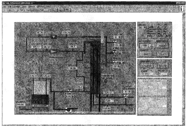
With the aim to calibrate steam flowmeters based on weight measurement of condensate, this system consists of a steam flow circuit and a cooling water circuit linked together by a shell and tube heat exchanger (see figure 1). The main components and operations of the system are as follows.

5

The steam is fed into the system by opening one of three valves shown by VRl-1 V, VMl-1 V and VR2-l V in the figure. This steam is in a saturated state the pressure (or temperature) of which is controlled by the opening position of the valve. The steam passes through the flowmeter to be calibrated shown by the symbol ~ before entering the shell side at the upper end of the heat exchanger, which is a vertical vessel. By transferring heat to the cooling water, the steam condenses in this shell side. The condensate drops to the bottom of heat exchanger and is discharged by the shell side outlet pipe and collected into a reservoir (see bottom left of figure 1).

Cooling water enters the lower end of the heat exchanger from an inlet pipe by opening the valve installed on it. Inside the heat exchanger, the cooling water splits and flows upward into 24 small tubes (not shown in details) then downward into 24 other tubes, connect together and leaves the vessel by the outlet pipe.

A scale is used to measure the weight of collected condensate as a function of time in order to calibrate the condensate flow rate. The height of the condensate within the heat exchanger is indicated by a sight glass (a vertical transparent tube shown on left side of vessel) and is controlled by the opening position of the valve VRl-lC, installed on the condensate outlet pipe. When this height becomes steady, the condensate outflow measured by the scale determines also the steam flow rate.

An integrated data acquisition system allows to record numerical values of selected operating parameters (such as pressure, temperature, condensate level, etc) at regular time interval. In our experiments, this time interval is set to 5 seconds ( see on the right side of figure 1) that give a reasonable number of sample data points linear fitting regression in deciding steady regimes.

2.2 Geometrie parameters of the beat excha:nger

Following parameters are needed for mathernatical development ofheat transfer process for controlling the steam pressure and the condensate level in the system (see figure 2).

~

1./ :;.---~-... ,

;/

.\

\

t

1

L

Conchmso. te wo. ter

c:*-

'

-l

1

Coollng wo. ter lnlet

-Jd-Figure 2 Shell and tube heat exchanger

- Shell diameter Ds = 0.3048m - Diameter oftubes D1 = 0.01905m

-Effective height ofheat exchanger L = 2.5m - Number of tubes N= 48.

CHAPTER3

DEVELOPMENT OF NEURAL NETWORK MO DEL FOR A CONDENSER SYSTEM

3.1 Introduction to Neural Networks

Artificial Neural Networks is a system loosely modeled on the human brain. The field goes by many names, such as connectionism, parallel distributed processing, neuro-computing, natural intelligent systems, machine learning algorithms, and artificial neural networks. It is an attempt to simulate within specialized hardware or sophisticated software, the multiple layers of simple processing elements called neurons. Each neuron is linked to certain of its neighbours with varying coefficients of connectivity that represent the strengths of these connections. Training is accompli shed by adjusting these strengths to cause the overall network to output appropriate results.

3.1.1 Basic unit of neural networks

The basic building block (unit) of neural networks, the artificial neuron, simulates the basic functions of natural neurons. The figure below shows the basics of an artificial

Xn

Figure 3

Y= f(I) 1 = (~wi*xi) + b Transfer

Sum +bias _function Output

Path Y

Each neuron receives various signais Xi coming from other neurons or directly from extemal inputs. These signais are processed within the actual neuron by a weighted summation I = (l.:wixi)

+

b where wi is a connection weight of the signal Xi, b is called the bias constant of the neurons. The weight coefficient Wi and the bias constant b of a neural network are the degree of freedom, to be determined by scaled conjugate gradient algorithm (see section 3.3.2). This sum is fed through a transfer function to generate a result Y = f(l) for the output path.

Three basic transfer functions are (1) all-or-nothing, (2) sigmoid and (3) linear. Only sigmoid and linear transfer functions are used for our heat exchanger process.

Y= f(I) Y= f(I) Y= f(I)

+1 +1

---,P...---0 I

0

-1 -1

( 1) all-or-nothing response (2) sigmoid response (3) linear response

Figure 4 Three basic transfer functions

3.1.2 General structure of artifidal neural networks

The developer must go through a period of trial and error in the design decisions be fore coming up with a satisfactory structure of artificial neural network for a particular system.

In a biological brain, each neuron can connect with up to 200 000 other neurons and the total number of connection is almost infinite. In an artificial neural network however, the connection structure is much simpler by grouping neurons into one input layer, one

9

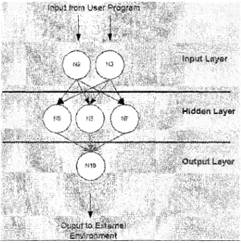
or several hidden layers and one output layer. The figure 5 shows a simple structure of a neural network.

Figure 5 Simple structure of a neural network

The input layer consists of neurons that receive input form the extemal environment. The output layer consists of neurons that communicate the output of the system to the user or extemal environment. There are usually a number of hidden layers between the input and output layers; the figure above shows a simple structure with only one hidden layer.

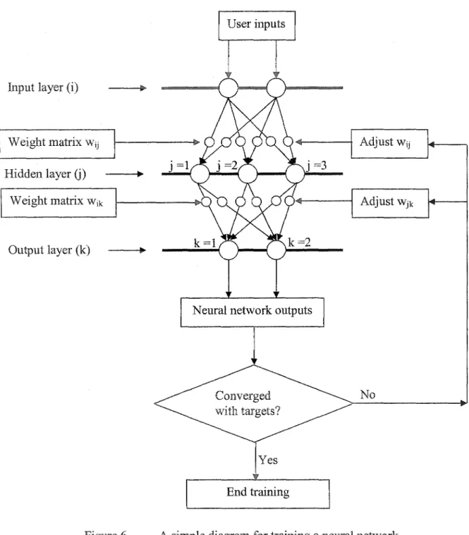
3.1.3 Training a neural network

Similarly to the brain that is trained from experience, each artificial neural network must also be trained before being used. The figure 6 shows a simple diagram for training a neural network. Training a neural network consists of giving several input data sets and the corresponding target output sets that are real output data obtained from experiments. A training method, which consists of a mathematical algorithm, is then

applied to adjust the weight matrices iteration by iteration until the network outputs satisfactory converge to the targets.

User inputs

Input layer (i)

W eight matrix Wij Hidden layer (j)

Weight matrix Wik Adjust Wjk

Output layer (k)

No

Y es End training

11

3.2 Preliminary analyses of the condenser system

The diagram of the condenser system in CTT laboratory of École de Technologie Supérieure has been shown in chapter 2 and reproduced in figure 1 for easy follow up purpose. Sorne preliminary analyses are needed before constructing appropriate neural networks. These analyses in elude (1) determination of input and output parameters; (2) choice of experimental data sets; (3) division of data sets into subsets for training, validating and testing the model; and ( 4) normalization of data.

3.2.1 Input and output parameters

Four input parameters of the actual condenser system and their limit operating are shown in table I.

Table I

Input parameters of condenser system

Input parameters Minimum and maximum values

Steam valve (VR1-1 V) Always closed (0%)

Steam valve (VR2-1 V) 5%- 100% opening

Condensate valve (VR1-Cl) 5.2%-6.5% opening

Inlet temperature of cooling water (CTl-lE) l19°F - 131 °F

There are also four output parameters which are :

-Steam pressure (indicated CP1-1 V) -Steam temperature (indicated CT2-l V) -Steam flow rate (shown by the symbol ~ -Condensate lev el (indicated DP 1-1 V)

3.2.2 Choice of experimental data

During system operation, each control valve (for steam and condensate) can be set up and changed manually or remotely from the computer. Each change of control valve openings takes about 10 minutes for the system to reach a new steady state regime. The transient or steady state regimes are simply observed and judged by watching recorded values appearing on the monitor of the computer.

Several experiments have been carried out on the condenser system, each one lasting for 2 to 6 hours. During each experiment, the opening position of the steam and condensate control valves are randomly changed many times after 5 to 60 minute intervals and data are recorded every 5 seconds for each measured quantity.

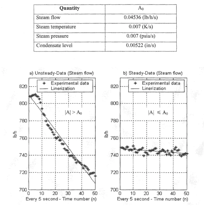
A Matlab program is created (see annex 2) to linearize each of four selected output quantities in function oftime for every data segment of 50 consecutive sample points (i.e every 250 seconds). The linearized functions are in the form

y=At+B

where t is the time, y is one of the four output quantities (steam flow, steam temperature, steam pressure and condensate level). A and B are the best fit constants for each data segment. The criteria used for deciding whether a data segment is steady, is the slope of the fitting line must be small:

- Unsteady if

lAI

>

Ao

- Steady if

lAI

~

Ao

where

lAI

is the absolute value of the slope and

Ao

is a given small value (see figure 7). The slope coefficient A0 that can be considered horizontal (steady) for the four output

~

..0

Table II

Maximum slope coefficient for steady data (Ao)

Qmmtity Steam flow

Steamtemperature Steam pressure Condensate level

a) Unsteady-Data (Steam flow) 820 _{--- - - Linerization}

+-

Experimental data

800 ... ~: 1 1 1 -~\-~---~---!---~---_{\ l. :} 1 1 \'":IF 1

i

\A\>Ao 780 760 --- -:---~---~---. -:---~---~---. -:---~---~---. -:---~---~---. -:---~---~---. 1 1 i 1 ' \ ' 1 1 : ·~-...:. : : :

\:"\

:

:

---r ----

~·~-

-t ---

~

---1 1 ~· 1 1 1 1 1

:

:

~ : 740 _____ ï _____ ' ï ____ _ ' ' ' a a 1 1 720 ---L---~---l---J-1 1 1 B '

\

700~--~--~--~--~--~ 0 20 30 40 50

Every 5 second- Time number (n)

..c

---..0 820 800 780 760 740 720

Ao

0.04536 (lb/h/s) 0.007 (KJs) 0.007 (psia!s) 0.00522 (in/s)

b) Steady-Data (Steam tlow)

+-

Experimental data Linerization ' ---~---~---~---~---' ' '

.

.

' ' \A\~ Ao : ' ' ' ---JI.---+---+---t---1 1 1 1 1 1 1 1 ' ' ' •----r---T---T---,---_{1 1} 1 1 ' 1 1 1 E ---L---1---l---~---' 1 1 1 ' ' 1 ' ' ' ' ' ' ' 10 20 30 40 50 Ever:i 5 second - Time number (n)

Figure 7 Examples of unsteady and steady data

The selection procedure for steady data is repeated until all experimental data are treated. The figure 8 shows an example of steady and unsteady data determined by the previous procedure applied to the steam flow during a 6-hour experiment.

3000 2500 2000 ..c ?i _"1500 1000 500 Figure 8

Choosing Steady-Data from experimental data of ste am tlovv

B l 1 1 1 - experimental data a 1 1 1 a ---~---y---r---,---y--• 1 1 1 - steady data ' ' ' ' ' ' ' _______ J ________ ! __ ' ' ' ' ' ' ---~---y--0 ' ' ---~---1--, ' _______ J ____ _

~

---~--~---~-~---' 500 1000 ' ' ---~---J ________ ! ________ , ________ J ________ t _ 1 1 • t 1 a ' ' ' ' _' ' '

---:---

~n

---

i ---

-1- ---

~-

- · ---K:

-'

'

'

j'

1 B 1 1

----~-

_____ j _______

l

----~

--- --- --- l_ 1 1 1 J 1 1 1 1 1 ' ' ' ' ' ______ J __ ' ' -~---1 ---~-' ' ' ' ' ' ' ' ' ' ' ' ' ' ' L-' ' ' ' ' 1500 2000 2500 3000 3500 4000 Every 5 second - Time number (n)

Steady and unsteady data for steam flow during a 6-hour experiment

Since the linearized procedure is independently applied to each one of the four output quantities, their steady state data may not occur at the same periods of time. By comparing four individual steady data sets (steam flow, steam temperature, steam pressure and condensate level), further elimination is finally done so asto keep only the time sets for which all quantities are simultaneously steady.

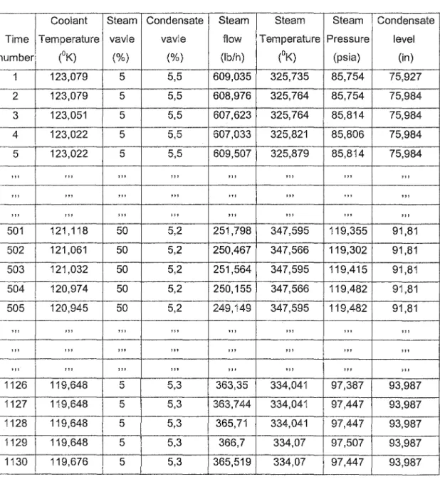
The total number steady data set is about 1130 which are consecutively renumbered. Sorne of these sets are shown in table III for three different combinations of steam and

15

condensate valve openings. Note that the inlet coolant temperature (second column of the table III) shows sorne fluctuations. However, it is always very small during any time segment of 250 seconds so that is always considered steady.

Table III

Steady state data sample points

Coolant Steam Condensate Ste am Steam Steam Condensate Ti me Temperature vavle vavle flow Temperature Pressure level number (oK) (%) (%) (lb/h) (oK) (psi a) (in) 1 123,079 5 5,5 609,035 325,735 85,754 75,927 2 123,079 5 5,5 608,976 325,764 85,754 75,984 3 123,051 5 5,5 607,623 325,764 85,814 75,984 4 123,022 5 5,5 607,033 325,821 85,806 75,984 5 123,022 5 5,5 609,507 325,879 85,814 75,984 '" "' "' '" "' "' "' '" "' "' '" "' ,, ,, '" ", "' "' '" '" "' '" '" _'" 501 121,118 50 5,2 251,798 347,595 119,355 91,81 502 121,061 50 5,2 250,467 347,566 119,302 91,81 503 121,032 50 5,2 251,564 347,595 119,415 91,81 504 120,974 50 5,2 250,155 347,566 119,482 91,81 505 120,945 50 5,2 249,149 347,595 119,482 91,81 "' "' "' '" ,, '" "' "' "' "' "' "' '" '" '" '" '" "' "' "' "' _{"' "' "'} 1126 119,648 5 5,3 363,35 334,041 97,387 93,987 1127 119,648 5 5,3 363,744 334,041 97,447 93,987 1128 119,648 5 5,3 365,71 334,041 97,447 93,987 1129 119,648 5 5,3 366,7 334,07 97,507 93,987 1130 119,676 5 5,3 365,519 334,07 97,447 93,987

3.2.3 Data division for testing neural network mode!

It is a common practice to split the available data into three sub-sets for training and validating each neural network model and for comparing different models. The basic idea is to withhold a small 'validation subset' to be used as a convergence criteria for each ANN model; (2) another small 'test subset' to be used to compare different models [ 4]; (3) the remaining subset for training each model.

In this study, the complete data is splited into three subsets in the following mann er : (1) the validation subset takes 25% of the data set and is composed of every fourth line of the overall set, i.e lines 4,8,12, ... ,1128; (2) the test set takes another 25% of the data set and is composed of lines 2,6,10, ... ,1130; and (3) the training set takes the remaining 50% ofthe overall set.

3.2.4 Data normalization

In any model development process, familiarity with the available data is of the utmost importance. ANN is no exception and data pre-processing can have a significant effect on model performance. Thus, before training, it is often to scale the inputs and targets so that they always fall within a specified range. In addition, the vmiables have to be scaled in such a way as to be commensurate with the limits of the activation functions used in the output layer. In Matlab, there are approaches to normalize original inputs and outputs as Min and Max, Mean and standard deviation and Principal Component Analysis. [6]

The functions premn.mx, postmnmx in Matlab are used to nonnalize the original inputs and outputs so that they fall within the [ -1,1] range. For each input or output quantity, designated by y, the minimum and maximum values are sorted from the data table ( designated by Y min and Y max) and the normalized value for each sample point is

17

Y

=

2

(y -

Y

miJ -

1 (Y max - Ynùn)

In the reverse manner, any quantity can be converted back to is ordinary values by :

3.3 Determination of ANN architecture

The architecture of a ANN consists of the number of layers, the number of neurons in each layer, the basic transfer function (sigmoid or linear) and how the layers connect to each other. Generally, the sigmoid type is used for transfer functions of ali neurons on hidden layers and the linear type is applied to neurons on the output layer.

3.3.1 General approach

There are two systematic approaches for determining optimal network architecture which are pruning and constructive approaches. [ 4]

Pruning approad.1 : The basic idea of pruning is to start with a network that is 'large-enough' to capture the desired input-output relationship and to subsequently remove or disable unnecessary neurons

Constructive approach : This approach optimizes the number of hidden layer from the opposite direction to pruning approach, starting with zero hidden layer. Hidden layer, their neurons and cmmections are then added one at a time in an attempt to improve model performance.

In this project, the constructive approach is selected for it reaches the optimal network with a relatively number of trial and error iterations.

3.3.2 Mathematical training algorithm

In the mathematical point ofview, training an neural network (NN) implies determining degree of freedom (Di) so that the errors between NN outputs and the targets are as small as possible. This is thus an optimization problem. The objective function for optimizing a NN problem is named the performance function p defined by the 'mean square error' of a certain number of a sample points.

where [D] the degree-of-freedom vector, YJk represents normalized output quantity j at a sample point k, ( j = 1 for steam flow, j = 2 for steam temperature, j = 3 for steam pressure and j

=

4 for condensate level),

Q

is called 'epoch size', i.e the number of randomly picked sample points within training data subset to be used to update the degree-of-freedom [D] and ejk represents the corresponding experimental value (target). If this perfonnance function is applied to aH sample points of the validation data subset, the result is denoted by pv[D] which is useful for cross-validation purposes to be explained later on.

If this performance function is applied to all sample points of the test data subset, the result is denoted PT which is useful for comparing different NN models.

\

\"'

Figure 9

19

-Pi-2

Illustration of optimizing two variables (D1,D2)

To start the optimization procedure, an initial point for degree of freedom must be given. In the present study, the first pointis set to be ali zeros: [Do]= [zeros].

At the beginning of iteration i, the degree of freedom [Di] are all known, and the training algorithm consists of choosing another set of degree of freedom [Di+l] so as giVe a smaller error :

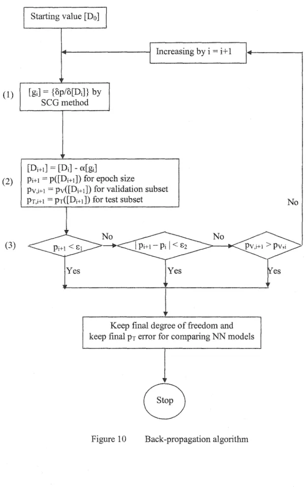
The back-propagation algorithm is the most commonly used for determining the next set [Di+Jl This algorithm is shown in figure 10 and explained as follows:

(1)

(2)

(3)

Starting value [Do]

1 + - - - J Increasing by i

=

i+ 1

[gi] = {ùp/ù[Di]} by SCGmethod

[Di+!] = [Di] - OL[gi]

Pi+t = p([Di+JD for epoch size

Pv,i+l = pv([Di+l]) for validation subset

PT,i+l = PT([Di+l]) for test subset _No

PV,i+l~

~Y_e_s

_ _ _ _ _ _ _ _ _ _ +Y-es __________

~!'es

l

Keep final degree of freedom and keep final PT error for comparing NN models

G

21

(1) Calculating the gradient vector [gi] (see figure 9) at point [Di], i.e [gi] = {op/o[Di]} at point [Di]. The present study uses a scaled conjugate gradient (SCG) method developed by Moller [ 11] to calculate gradient vectors.

(2) Calculating the next point [Di+l] on the negative gradient direction by equation

where ais a constant determining size of the next step (a= 0.5 in this study). A smaller the size step gives the better accuracy but takes more iterations and more calculation time (see figure 10).

(3) Testing convergence criteria :

Three convergence criteria are sequentially used in order to stop the iterations.

- when training error has reached sufficiently small value

Pi+I < s1 (for each epoch size

Q

= 75 sample points)

- or when training error is not changed significantly :

1

Pi+J- Pi

1<

!':2 (for each epoch size Q = 75 sample points)

- or when the validation error starts to rise

pv,i+l > pv,i (for ali validation subset, about 280 sample points), the later is called the 'cross-validation' criteria, which is useful for cases in which the first two criteria can not be met.

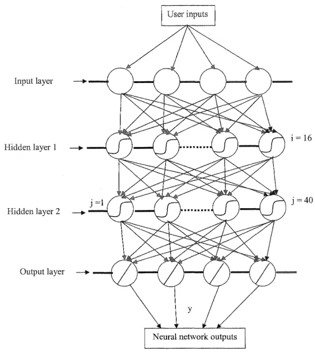
3.3.3 Resulting NN for steam condenser system Input layer i = 16 Hidden layer 1 Hidden layer 2 Output layer

Figure 11 Neural network model of condenser system

A Matlab program is written for training NN models for our steam condenser system (see mmex 2). The program contains the function 'trainscg' already developed (by Matlab)

23

using the previous described algorithm. It also contains four manually given parameters which are (1) epoch size Q, (2) leaming rate a, (3) number of hidden layers and (4) number of neurons in hidden layers.

Each combination of these parameters takes about 1 to 2 hours computer time before meeting the convergence stopping criteria (using a 900Mhz Pentium III computer). This pro gram is applied several times by changing one of these parameters each time before obtaining the most acceptable NN model for the condenser system. The retained NN model is summarized as follows: (see figure 11)

Epoch size Q = 75 sample points which are repeated with the training data set until the

convergence criteria are met;

- Leaming rate: a= 0.5;

- Number of hidden layers: 2;

- Number of neurons: 4 for input layer, 16 for the first hidden layer; 40 for the second hidden layer and 4 for output layers.

- Transfer function: sigmoid function for two hidden layers and linear function for output layer

The best values of weight matrices and bias constants are presented in Annex 1, which comprise a 16x4 weight matrix [w1] and a 16xl bias vector [bi] for information going from the input layer to the first hidden layer, a 40x16 weight matrix [w2] and a 40xl bias vector [b2] by going from the first hidden layer to the second hidden layer, a 4x40 weight matrix [w3] and a 4xl bias vector [b3] by going the last layer to the output layer.

3.4 Application of retained neural network.

All the parameters of the retained NN model (weight matrices Wij and bias vectors bi) have been kept in text files w1.txt, w2.txt, w3.txt, b1.txt, b2.txt, b3.txt. In order to allows users to predict output results of the condenser system (i.e steam flow, pressure, temperature and condensate height) for a certain given input condition (i.e valve openings), another program is written (see annex 2) to execute following straight forward steps:

(1) Reading files for weight matrices Wi and bias vector bi.

(2) Reading a set (x) of 4 input quantities to be treated (2 steam valve opemngs, condensate valve opening and coolant temperature). Each input must faU with the operating range of the system, already mentioned in Table 1.

(3) Calculating output values by transfer functions of the retained NN model shown in figure 11. The four quanti ti es of the output vector y are un-normalized back to their real units (lb/h for steam flow, psi a for pressure, Kelvin for temperature and inch for condensate height) and their calculation can be represented by the form

where f1,

6

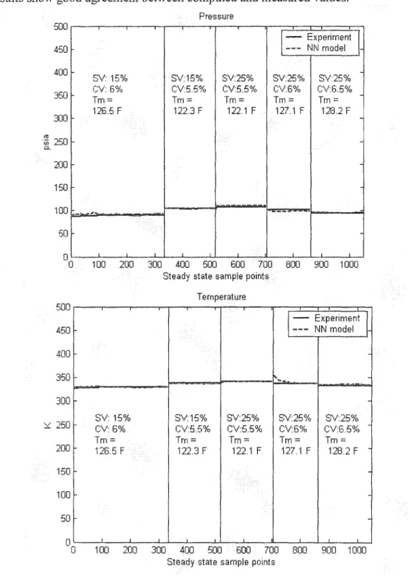
and f3 are transfer functions of the first hidden layer, the second layer and the output layer of the NN model. To implement application exarnple using this prograrn, another experiment has been carried out independently from the training data and the program is applied for calculating predicted outputs for steady data of this experimental outputs and those given by NN model is presented in figure 12 for several input conditions (steam valve opening indicated by SV, condensate valve opening

25

indicated by CV and the average temperature of cooling water indicated by T rn)· The results show good agreement between computed and measured values.

Pressure 500 450

1=

Experiment

J

NN rnodel 400 SV: 15% SV:15% SV:25% SV:25% S\/:25% CV': Gqt;) CV:5.5% CV:5.5% C\/:6% C\1:6.5% Tm= Tm= Tm= Tm= Tm= 350 126.5 F 122.3 F 122.1 F 127.1 F 128.2 F 300 ,., Q) 250 Q_ 200 150

---

" 100 50 0 1J 1 00 200 300 400 500 600 700 BOO 900 1 DOO

Steady· state sample points Temperature 500 450

1=

Experiment

1-NN model 400 350 "~ 300 SV: 15% SV:15% S\1:25% SV:25% S\1:25% CV: 6% CV:5.5% CV:5.5% C\1:6% CV:6.5% ::,:: 250 Tm= Tm= Tm= Tm= Tm= 200 _{126.5 F 122.3 F 122.1 F 127.·1 F 128.2 F} 150 100 50 0 0 1 00 200 300 400 500 600 700 800 900 1 000

Steady state sample points

Condensate leve! 500 450

1=

Experiment 1-NN mode! 400 350 300 SV: 15% SV:15% S\1:25% SV:25% S\1:25~10 CV: 6% C\/5.5% C\1:5.5% C\1:6% C\1:6.5% -~ 250 _{Tm= Tm= Tm= Tm= Trn =} 126.5 F 122.3 F 122.1 F 127. ·J F 128.2 F 200 150 100 ~ .... ,.,...;.~~~11? .... ..-bo;.IT'""""-#"""d'/""-

r---

1-.,

-... ,... .... ---"""---~-50 0 0 1 00 200 300 400 500 600 700 800 900 1 000

Steady state sample points Steam flo1.•1 3000

1=

Experiment

1

Nf\J mode! 2500 _ooot'_ ... """"'""'"111 2000 -'bo'!aoo...., ...

"':.---""-"""·"'---

.. ..c ~ 1500 1000 L~ ,.

________

-,...-.,., ____ SV: 15% S\1:15% S\1:25% S\1:25% S\/:25% 500 CV: 6% C\1:5.5% C\1:5.5% CV:6% C\1:6.5% Tm= Tm= Tm= Tm= Tm= 126.5 F 122.3 F •122.1 F 127.1 F 128.2 F 0 0 1 00 200 300 400 500 600 700 BOO 900 1 000

Steady state sample points

27

3.5 Conclusion

According to the results shown in the previous numerical application, it is seen that the artificial neural network (ANN) model presented in this study performs successfully for the condenser system. The main advantage of the ANN approach is the automatic selection for the algorithm that relates the inputs to the outputs. Also, the approach could adapt itself to assemble the desired output with a training input sample. It allows multiple input versus multiple output relationship. The main drawback of the ANN model is that it can not explain how the quantities are related to each other

A way of overcoming this drawback is to develop a physical model for the condenser system, which is the subject of the next chapter.

A PHYSICAL MODEL FOR THE STEAM CONDENSER SYSTEM

4.1 Objective

A physical model is herein developed for the same steam condenser system previously described. This approach is based on the conservation of mass and energy. The physical model has the same objective as the NN model, which is to predict output quantities in function of inputs. It differs from the NN model by several aspects including the following

(1) The physical model describes the response of the system by using equations derived from physicallaws.

(2) The physical model directly takes real output quantities such as pressure, temperature, heat transfer, mass flow, etc ... as degrees of freedom (DOF), which NN model use meaningless quantities such as weight coefficients, bias constants or transfer functions.

(3) The physical model dynamically describes the system from an initial condition through out transient states until a new steady state condition is reached, while the NN mo del just treats steady state conditions

( 4) The number of DOF of the physical madel depends on the number of discretion 'control volumes', such as described in the next section.

29

(5) The coolant water flow rate, mw is not considered in NN model for it is practically unchanged during all operating conditions but is now considered in physical rnodel for it simply appears in conservation equations.

( 6) The physical model takes saturated ste am conditions into account so that the steam pressure P s and temperature T s are related to each other by the saturated steam table,

while NN model treats them like two independent quantities.

4.2 Modelling . . . - = - - - l Ts

P.

~C.V3

Steo.n) 862KPo. T H Figure 13

1

1"1 _'1'.'

q3

vo.l ve tuloes

Discretion of control volumes of condenser system

The condenser system is divided into control volumes (C.V) and equations are developed for physical quanti ti es at boundaries of these volumes. In general, increasing the number of CV s gives better results but involves more equations to be developed and more calculation time. In the present study, condensate volume is divided into two equal control volumes (C.Vl and C.V2) and the steam above the condensate is taken as one control volume (C.V3 in figure 13). There are thus five corresponding CVs on tube side denoted by six boundary temperatures T1 to T6 in figure 13.

In developing mathematical equations for this model, the following parameters are needed, sorne of them being constant and the other being variables in function oftime.

The constant parameters are composed of geometrie quantities and input quantities of the system. The geometrie quantities are shell side and tube side dimensions such as inside diameter and total effective length of shell (Ds and L in figure 13), number of tubes (N = 48) and their inside and outside diameters (Dt and Dt0 ). The input parameters are defined as the physical quantities that can be directly adjusted. In this model, the input quantities are :

• Ks ... steam valve proportionality constant corresponding to a valve openmg, (kg/s/Pay')

• Kc ... condensate valve proportionality constant corresponding to a valve opening,

• T 1 •. .inlet coolant temperature, and

• rn w for flow rate of cooling water on tube si de.

The variable parameters in function of time include all quantities that are not directly adjusted but related input quantities via physicallaws. They are :

31

e ms for incoming steam flow rate at top of shell, (kg/s), the dot symbol above letter m being used to designated the derivative dm/dt with respect to time,

e Ps and Ts for saturated steam pressure (Pa) and temperature (°K) in C.V3,

e mcond and mc for condensation rate at boundary C. V3 to C. V2 and

intermediate flow rate from C.V2 to C.Vl, respectively

.

e rn valve for outflow of condensate at bottom of shell

• Tc1 and Tc2 for average temperatures of condensate m C.Vl and C.V2,

respectively

e H1, H2 and H3 for heights of corresponding control volumes (Noted that H1 + H2

+ H3 = L is constant, and H1 = H2 = H/2, half of condensate height, variable with

time).

e T _1, T _{2, ... ,} T ₆ for temperature of cooling water inside the reversed U tubes at

boundary levels of control volumes

e q1, q2 , ... , q5 for heat transfer rates from shell side CVs into tube side CVs (see

figure ... )

• Physical properties such as enthalpies of steam and condensate (hs, heand,

... W/m2/K), specifie heats (Cp, J/kg/K), and densities of steam, condensate and water (p, kg/m3).

4.3 Matb.ematical equations of the model

The mathematical equations of the previously described model are presented in this section under 5 categories : - continuity equations (or conservation of mass) in control volumes of shell si de; - energy equations in CV s of shell si de; - energy equations in CV s of tube si de; -heat transfer equations across tube wall; and miscellaneous relationships.

4.3.1 Continuity equations

The general princip le ofthe continuity of mass in a control volume states that :

(

Rate of input] _(Rate of output]

=

(Rate of accumulation]

rnass rnass mass

For each of two control volumes of condensates (C.Vl and C.V2), this principle gives following equations. • • p AdH mc-mvalve

=

1 1 dt (4.1) • • PoAdH7 lllcond- ille

= -

-dt (4.2)

where A= n

n; -

N

*

n

n;o

which means the net cross-section area of the shell side

4

4

For control volume 3 (C.V3), the fluid is saturated steam, so that the continuity equation of saturated steam must be used [14], which is

33

(4.3)

On the tube side, the cooling water flow rate (rn w ) is practically unchanged for all

operating conditions. Furthermore, water is treated as incompressible so that it is reasonable to assume that this flow rate is constant over the entire volume on tube side. This value is mw= 0.65 kg/s which is determined from experimental data and applies for all test conditions in this study.

4.3.2 Energy equations of control volumes on sheU side

The general principle of the energy balance in a control volume states that (see figure 14)

(rate of _{inflow enthalpy - outflow enthalpy - to tube side} ) (rate of

J

(rate of heat loss )

₌

( rate of _{stored energy}

J

Figure 14 Inflow enthalpy C.V Outflow enthalpy Heat loss

For control volumes 1 and 2 in which the following mater is condensate, this principle gives two following equations :

• • pAHC d(T)

*

h

*

h C T

* (

) _

1 1 pl cl IDe c - I D valve valve-q_{1 -} q_{5 -} pl cl IDe- ID valve

-dt (4.4)

(4.5)

For control volume 3 (saturated steam), a simpler energy equation is obtained by using the heat of vaporization hfg (J/kg), property of saturated steam, an intrinsic [ 13] :

4.3.3 Energy equations of control volumes on tube side

1 1 1

j

!Outflow enthalpymw CpTk+l) •.•••••••. ,1 Cooling

t

water flow 1 Heat gain qk

1 ... 1Inflow enthalpy rn w Cp T~c) 1 1 1

Î

1 1 1 1 1 1 1 1 1

Figure 15 Typical control volume k on tube side (k = 1, to 5)

(4.6)

Applying the general principle of energy balance for control volumes on tube side gives much sirnpler equations because the tube side flow is considered constant (steady). The five equations for control volumes on tube side are represented by :

35

(4.7 to 4.11)

Note that for simplification purposes, the specifie heat of cooling water (Cp) 1s considered constant in each control volume.

4.3.4 Heat transfer equations across tube waUs

Shell side CVi

(Tcj)

k (Heat trans fer)

Figure 16 Heat transfer across wall from shell CVi to tube CVk

The previous equations are not sufficient to describe the relationships between shell side and tube side because the heat transfer coefficients across tube wall are not taken into account. This section completes this kind of relationships.

The figure 16 shows the main parameters involved in the heat transfer phenomenon across tube walls between a tube control volumes (CVk with k =1, 2, ... , 5) and the corresponding shell control volume (CVj withj =1, 2 or 3).

Applying the 'log-mean temperature difference' heat transfer equation developed for shell-and-tube heat exchanger [13], gives five equations of the same following form.

(4.12 to 4.16)

where k designates tube control volume number (k = 1, 2, ... , 5) and j designates

corresponding shell control volume (for example, if tube side k =1 then shell side j = 1, if tube si de k = 4 then shell si de j = 2, etc ... , see mo del shown in figure 12), and U A₁ is 'the overall heat transfer coefficient' across 48 tube walls in the control volume CVj.

The overall heat transfer coefficient (UAj) depends on the number of tubes (N=48), tube length in the control volume (Hj), tube diameters (Dt and Dt0 ), convection coefficients

ho

and hi at outside and inside of tube wall, (W/m2lK) and thermal conductivity K of tube material (W/m/°K).

37

It is noted that in the expression of coefficient UA3 for shell control volume 3, the

convection h03 due to steam condensation on outside tube wall is very large so that the

ratio 1Ih03 is neglected, and the tube length is approximately equal to twice the height H3

due to U bend.

4.3.5 MisceHaneous relationships

To complete the required number of equations for the unknown parameters in above equations, following miscellaneous equations are needed.

e Relationship between water flow and convection coefficient hi inside tubes [13]: This relationship has two forms depending on whether the flow is laminar or turbulent, indicated by the Reynolds number Rek :

4*mw Rek

=

_*_D_*-'-.-re t llk

where 1-Lk is the absolute viscosity (N.s/m2) of cooling water inside CV1c,

- IfRe1c < 2300: the flow is laminar, then ~ik = 3.66KJDJ

0 023KRec415_lPr04

-IfR~ > 2300: the flow is turbulent, thenh;k = · k

Dt

where Pr is the Prandtl number of the cooling water at the corresponding temperature

e Relationship between condensate flow and convection outside tube [13]: The Reynolds number of condensate flow outside the tubes is calcu1ated by

4*m *D

Re.

=

1 11

j

=

1 or 2, shell CVj

1

n*(D2 _s -ND2 _to )*1t. _{r- J}

where mi is the average condensate flow rate in the control volume j; and Dh is the 'hydraulic diameter' of shell si de, defined by

D2 ND2

D - s to

I

-l Ds +NDto

The condensate flow is always laminar, the convection coefficient ho is given by

h .

=

(0 664

*

Re05

_*

_{Pr(ll3) )/D}

0] • J J h

Relationship between saturated pressure and temperature

For saturated steam, the pressure P s and the temperature T s are dependent to each

other. This relationship can be represented by the general form.

(4.17)

However, this function is practically replaced by a steam table. • Height relationships

39

(4.18)

(4.19)

(4.20)

Characteristics equations of condensate valve and steam valve

The relationships between a valve opening condition (e.g 5.5% steam valve with 15% condensate valve) and other parameters of the model (P0 , P5 , Pc, Ks and Kc) are

introduced under the characteristics equations of valves as follows :

(4.21)

Condensate valve:

~vatve = Kc~pc

-Patm (4.22)

where P 0 is the pressure of steam source outside the condenser system (P 0 = 862kPa,

constant), Patm is the atmospheric pressure (the condensate tank is open to atmosphere ), and Pc is the pressure of condensate at bottom of heat ex changer which is slightly higher than the steam pressure by the height of condensate :

Ks and Kc are the valve coefficient (kg/s/Pa112), experimentally determined

The numerical values of these coefficients for nine combinations of valve openings are shown in table IV.

Table IV

Valve coefficients (Ks and

Kc)

corresponding to opening conditions

~

15% 25% 50%

c

6.5% Ks =12.18 Ks =17.45 Ks =23.45 Kc =10.01

Kc

=9.9 Kc =10.2 6% Ks =11.52 Ks =14.98 Ks =17.49

Kc

=7.24

Kc

=7.26 Kc =7.48 5.5% Ks =8.72 Ks =9.625 Ks =10.49

Kc

=3.93

Kc

=3.85 Kc =3.92

4.4 Equation system solving

The previous section gives a set 22 differential-algebraic equations (DAEs), five of which are ordinary differentiai equations for the pararneters Tel, Tcz, Ps, H1 and Hz. (see equations (4.1) to (4.5) and the remaining are algebraic equations). These equations are

. . .

sufficient for determining 22 unknowns, which are 4 flow rates (ms , fficond , mc and

.

ffivaive), 8 temperatures (Ts, Tel, Tcz, T2 to T6), 2 pressures (Ps and Pc), 5 heat transfer

rates (q1 to q5) and 3 heights (H1, Hz and H3).

A program has been written to solve this DAE system using the function 'ode15s' of Matlab (see mmex 2). This function already includes an algorithm for automatically adjusting the time interval At so as to give satisfactory convergence from an initial condition until the corresponding state condition is reached.