HAL Id: hal-01412950
https://hal.archives-ouvertes.fr/hal-01412950
Submitted on 9 Dec 2016
HAL is a multi-disciplinary open access
archive for the deposit and dissemination of
sci-entific research documents, whether they are
pub-lished or not. The documents may come from
L’archive ouverte pluridisciplinaire HAL, est
destinée au dépôt et à la diffusion de documents
scientifiques de niveau recherche, publiés ou non,
émanant des établissements d’enseignement et de
CT-Mapper: mapping sparse multimodal cellular
trajectories using a multilayer transportation network
Fereshteh Asgari, Alexis Sultan, Haoyi Xiong, Vincent Gauthier, Mounim El
Yacoubi
To cite this version:
Fereshteh Asgari, Alexis Sultan, Haoyi Xiong, Vincent Gauthier, Mounim El Yacoubi. CT-Mapper:
mapping sparse multimodal cellular trajectories using a multilayer transportation network. Computer
Communications, Elsevier, 2016, 95, pp.69 - 81. �10.1016/j.comcom.2016.04.014�. �hal-01412950�
CT-Mapper : Mapping Sparse Cellular Trajectories to
Multimodal Transportation Network
Fereshteh Asgaria, Alexis Sultana, Haoyi Xionga, Vincent Gauthiera,∗, Mounim El-Yacoubia
aSAMOVAR, Telecom SudParis, CNRS, Universit Paris-Saclay
9 rue Charles Fourier 91011 Evry, France
Abstract
Mobile phone data have recently become an attractive source of information about mobility behavior. Since cell phone data can be captured in a passive way for a large user population, they can be harnessed to collect well-sampled mobility information. In this paper, we propose CT-Mapper, an unsupervised algorithm that enables the mapping of mobile phone traces over a multimodal transport network. One of the main strengths of CT-Mapper is its capability to map noisy sparse cellular multimodal trajectories over a multilayer transporta-tion network where the layers have different physical properties and not only to map trajectories associated with a single layer. Such a network is modeled by a large multilayer graph in which the nodes correspond to metro/train stations or road intersections and edges correspond to connections between them. The mapping problem is modeled by an unsupervised HMM where the observations correspond to sparse user mobile trajectories and the hidden states to the mul-tilayer graph nodes. The HMM is unsupervised as the transition and emission probabilities are inferred using respectively the physical transportation proper-ties and the spatial coverage of antenna base stations. To evaluate CT-Mapper we collected cellular traces with their corresponding GPS trajectories for a group
∗Corresponding author
Email addresses: [email protected] (Fereshteh Asgari),
[email protected] (Alexis Sultan), [email protected] (Haoyi Xiong), vincent.gauthier@telecom-sudparis (Vincent Gauthier),
of volunteer users in Paris and vicinity (France). We show that CT-Mapper is able to accurately retrieve the real cell phone user paths despite the sparsity of the observed trace trajectories. Furthermore our transition probability model is up to 20% more accurate than other naive models.
Keywords: Mobile phone, Mobile networks signaling, Multimodal
transportation network, HMM, Unsupervised learning, Mobile trajectories mapping, Intelligent transportation systems
1. Introduction
Macroscopic analysis of the traffic flow in large metropolitan areas is a chal-lenging task. This is especially true when multiple transit authorities are in charge of different transport networks (road, train, subway). Due to the lack of a common source of information across these transit systems, it is often hard for city authorities to grasp a unified view of mobility patterns. In this context, mo-bile phone data have recently become an attractive source of information about mobility behavior. Thanks to the ubiquitous usage of mobile phones, mining mobile phone data becomes a promising way to understand multimodal human mobility [1, 2, 3] ranging from identifying a mobile user daily path to recording transportation usage (e.g., taking train, metro, bus, etc.) in a large metropoli-tan area. Traditional approaches of mobility studies used GPS to accurately sense spatial data with a localization error bound ≤ 50m. Although they en-sure the collection of fine-grained mobility trajectories (as shown in Fig. 1b), GPS-based data collection has two main drawbacks: first, it causes high en-ergy consumption, and second, it is constrained to a limited group of users (e.g. taxi drivers [4] or a group of car drivers [5]). GPS sensing, therefore, is not suitable for collecting large-scale data from metropolitan area populations. By contrast, cellular data provided by network operators does not suffer from these issues, and has become recently, as a result, a new source of mobility informa-tion. Signaling information from mobile network operators (CDRs -Call Data Records-) has been used as a valuable source of mobility information for large
scale population [3, 6, 7].
Localization of mobile phone users with antennas (i.e., cellular towers), nonetheless, provides only coarse-grained mobility trajectories at antenna level, with a varying localization error of hundred meters in densely populated cities, and within several kilometers in rural areas [3]. Given the resulting cellular
mobility trajectories (i.e., a sequence of antenna id s) and the location of each
antenna as shown in Fig. 1c, it might be difficult to observe the road or metro station that the user passes by (as shown in Fig. 1a).
In order to collect cellular mobility trajectories using mobile phones, previous works [6, 3] usually extracted the trajectories from Call Detailed Records (CDR), where the CDR of a user restores the antenna id and the time-stamp of each of his/her mobile calls. To understand human mobility, these works were mostly limited to aggregating the trajectories from a user’s long-term CDR data in order to determine the frequently-visiting locations and the visiting time (e.g., the park he/she usually passes by during the 07:00–09:00 window of working days). As such, the techniques proposed by previous works are not suitable for estimating the precise mobility trajectories on the road/transportation network using the CDR cellular trajectories.
Furthermore, one sample of CDR data (i.e., one call record) can be obtained only when the user places a call, making human mobility data between two consecutive calls irretrievable, especially when the time duration between the two calls is long (e.g., the inter-call mobility between the two calls in Fig. 1d). Thus, even though it has been studied widely, CDR is unlikely to be a good data source for the trajectory mapping problem. Considering the time sparsity drawbacks of CDRs, we use, in this work, a new passive capturing technique to efficiently extract the position of the base stations the mobile phone is connected to. This technique analyzes the signaling channel of the data mobile network in order to extract base station locations. This way of capturing the mobility of users is salable and provides a higher sampling rate than CDR-based sensing.
The sparse cellular trajectories are collected and provided upon the request of the experiment participants to the network operator. Considering privacy
(a) Road Trajectory (b) GPS Trajectory
(c) Cell Trajectory (Full) (d) CDR Trajectory
(e) Sparse Cell Trajectory
Figure 1: A user’s trip from Airport CDG to city center of Paris: The road trajectory consists of the sequence of roads that the user passes-by; The GPS trajectory is sampled in minute based frequency; The Cellular trajectory (Full) records each cell tower the user passes-by; The CDR trajectory reports the location of the user’s each call during the trip; The Sparse Cellular trajectory is sampled every 15 minutes
issues [8], the network operator localizes each mobile user using an antenna id, and further records each user’s antenna id with time-stamp periodically
(e.g., every 15 minutes in our study). Compared to the user’s real trip (in Fig. 1a), the sparse cellular trajectory (in Fig. 1e) partially measures the user’s mobility with coarse-grained localization. The objective of our work is to map each sparse cellular trajectory 1 into the multimodal transportation network, in order to obtain the sequence of network nodes that the user passes by. For example, given the cellular trajectory shown in Fig. 1e and the transportation network of the Paris metropolitan area shown in Fig. 2, our goal is to recover the sequence of nodes of the real trip shown in Fig 1a.
The common approach for mapping cellular trajectories into the metropoli-tan transportation (usually road) network is to first collect a large amount of cellular trajectories and then to manually label each cellular trajectory with the corresponding intersection sequence, an intersection being a graph node associ-ated with a junction between two roads. The next phase is to train a supervised
mobility model (e.g., HMM) using the labeled cellular trajectories, in order to
build a probabilistic model mapping antenna id sequences to intersection se-quences. After training, given a new user cellular trajectory, the supervised model predicts, as the mapping result, a sequence of intersections, having the maximal likelihood of generating the antenna id sequence. However, obtaining the labeled cellular trajectories to cover the road/transportation networks and all cellular towers of a metropolis is not practical, as it costs too much human efforts for trajectory collection and labeling. We propose, in this paper, to solve the cellular trajectory mapping problem using an unsupervised mobility model, that does not require collecting and labeling any trajectories.
Given the above examples and target research goals, the key issues in de-signing the unsupervised mobility model include:
1) Given the antenna id sequence in a cellular trajectory, retrieve the
se-1In the rest of paper, we use the term ”cellular trajectory” and ”sparse cellular trajectory”
quence of road/rail intersections that the user passes by given a database storing the multimodal transportation network - The transportation network
cov-ering and connecting multiple types of transportation modes (e.g., rail, metro, highway , etc.) is named multimodal transportation network [9], in which each node is either a road intersection or a station of a rail transportation mode (i.e., subway, tramway and train), and each edge is a connection between intersections (e.g., the pathway connecting a metro station and a bus stop). Obviously, it is nontrivial to extract the precise user path from the multimodal transportation network using the antenna id sequences.
The cellular trajectory might come from multiple transportation systems nearby each corresponding antenna and in different layers (underground, ground and trestle). To overcome this issue, it is necessary to build a comprehensive database storing all the intersections of the multimodal transportation network, where we can accurately retrieve the surrounding intersections of each antenna. In this work, open data provided by OpenStreetMap (OSM) and the National Geographic Institute (IGN) are used to extract the multimodal transportation network of Ile-de-France (Paris and vicinity). This region is characterized by a high diversity of public transportation modes (tram, RER, train, bus) that have each particular specifications. Therefore, building a multimodal transportation network to study individuals’ mobility requires a clear understanding of the multimodal network complexity. The multimodal transportation network is modeled in this work based on the concept of ’cross-layer’ links that connect each two nodes where users can switch transportation modes.
2) Given an observed cellular trajectory, compute the most-likely
inter-section sequence over the multimodal transportation network - It is difficult
to search the most-likely intersection sequence from the set of intersections, due to the following reason:
Likelihood Computation: In order to search the most-likely intersection sequence, given an observation sequence, we need to calculate the likelihood of each node given the cellular trajectory. While the traditional supervised HMM mobility model harnessing the statistics of labeled cellular trajectories
(i.e. emission/transition probabilities) is usually used to estimate the likelihood, we propose an unsupervised HMM that does not leverage labeled data. Rather it proposes a method to calculate the likelihood using the topological properties
and other information of the transportation network. In other words, the HMM
parameters are automatically derived in an unsupervised way based on a priori knowledge of transportation network properties.
In summary, the main contributions of this work are:
• We propose to study the problem of mapping cellular trajectories to the multimodal transportation network, in order to obtain the precise mobility
of the users. To the best of our knowledge, this is the first work addressing these issues. In particular, rather than mapping cellular trajectories using the supervised mapping algorithms with labeled mobility data, we pro-pose to use an unsupervised mapping algorithm leveraging on topological properties of the transportation network, so as to eliminate the tedious human labeling efforts in building the mobility model.
• We propose an unsupervised trajectory mapping algorithm, namely CT-Mapper, which maps cellular location data over the multimodal
trans-portation network. The multimodal transtrans-portation network database was built using different references of geospatial resources. The mapping algo-rithm is modeled by an HMM where the observations correspond to user cellular trajectories and the hidden states are associated with nodes of the multilayer graph. Transition probability and emission score were modeled based on topological properties of the transportation network and the spatial distribution of antenna base stations. Viterbi decoding algorithm helps reduce the complexity of finding the best match which might enable us to deploy our unsupervised mapping algorithm on large scale mobility data sets in order to estimate multimodal traffic in metropolitan areas.
• We collect real cellular trajectories of a group of users in the Paris
metropoli-tan area with the help of a French telecom operator, then evaluate our mapping algorithm using the data. Through the extensive evaluation
with cellular trajectories covering more than 2500 intersection nodes and 3 physical layers , 1000 metro and subway stations, we show that our al-gorithm maps the cellular trajectory onto the multimodal transportation network of the Paris metropolitan area and with good accuracy given the sparsity of user cellular trajectories. This algorithm also achieves up to 20% higher accuracy compared to a baseline approach, that exploits for unsupervised HMM parameter estimation, the complexity and topology of the multilayer network, without considering the transportation properties of network edges.
The rest of this paper is structured as follows: Sec.2 presents related work. Sec. 3 gives an overview of the proposed system. Sec. 4 presents the details of the unsupervised estimation of HMM parameters and explains how the two main probability distributions used for mapping are derived. In Sec. 5 , we evaluate our proposed algorithm and the paper ends by a discussion and a conclusion in Sec. 6.
2. Related Work
2.1. General Human Mobility Models
A considerable amount of Human Mobility studies have been devoted to analyze trajectories of individuals based on their traces. Spatial characteristics such as center of the mass, radius of gyration and statistical characteristics re-vealed a number of scaling properties in human trajectories: Gonzalez et al in [10] and Brockmann et al [11] showed a truncated power-law tendency in the distribution of jump length. It was observed that most individuals travel only over a short distance, and there is only a few who travel regularly over hundred kilometers. Further studies [12, 10] showed that travel patterns collapse into a single spatial probability distribution, indicating that, despite the diversity of their travel history, humans follow simple reproducible patterns. In addition, statistical analysis confirms that individuals’ movement follows spatio-temporal patterns [5, 13, 14] which can help defining mobility models. In all mentioned
studies, multimodal mobility aspects were not taken into account. One objec-tive, in this work, is to investigate the mobility patterns of trajectories through the multimodal transportation network and to explore how these patterns are affected by the multiplicity of the layers of the network. Early mobility studies relied on expensive data collection methods, such as surveys and direct obser-vation. Trajectories were mostly defined as Origin-Destination (OD), and were mapped over the desirable graph to retrieve an optimal path solution which is usually the shortest path between the Origin and Destination [12, 15, 5, 13]. Al-though recent studies have been trying to infer the traffic flow using additional traffic data [16], they still fail to retrieve the real path taken by individuals.
2.2. Mapping Algorithms
Along with mobility studies, applications such as navigation systems, traffic monitoring and public transportation tracking, used GPS data to track indi-viduals or any moving object [17, 18, 19, 20, 21, 22]. A variety of statistical approaches such as Expectation Maximization (EM) [22], Kalman Filter [20, 21] and Hidden Markov Model (HMM) [23, 17, 18, 19, 24] were used to map noisy sequential location data over transportation networks. Most of these mapping algorithms have used GPS data as they provide accurate location data with an error of about 50 meters. Moreover, using labeled data, supervised mod-els were considered and trained to optimize model parameters in an automatic way. Once the models are trained, they are used to find the most likely path in the network assigned to sequences of noisy location data. However, most of these mapping algorithms were developed to map noisy data over road networks without considering other mobility modes.
2.3. Human Mobility Modeling with CDR Cellular Trajectories
Recently, because of the expeditious growth of mobile phones, Call Data Records (CDR) have been providing great data sets for human mobility studies as they are collected continuously for all active cellular phones. CDRs, however, have two significant limitations: first, they are sparse in time because they are
generated only when a phone engages in a voice call or text message exchange; and second, they are coarse in space and less precise than GPS location data, because they record location only at the granularity of a cellular antenna (with an average error of 175 meter in dense populated areas and up to 2 kilometers in less denser areas). Nonetheless, the fact that almost the entire population is already equipped with cell phones [3] allows for studying important aspects of individual mobility such as inferring transportation modes. Cellular network data were, for instance, used to classify different transportation modes for long-distance travels [3, 2]. Thiagaran et al. in [17] used cellular signal data with combination of cellphone sensors to develop a supervised mapping algorithm in order to overcome the limitation of GPS data. While previous works have used cellular data to map long trajectories, this work proposes an unsupervised map-ping algorithm that maps the sparse cellular trajectories over the multimodal transportation network in the Paris metropolitan area. This approach could be used for large scale smart-phone users for further studies in traffic estimation. Such a mapping is important for the development of smart cities and smart mobility.
Studies of smart cities in the past were limited to analyzing multimodal transportation networks without considering large scale real mobility data. The main goal of multimodal mobility studies is to improve public transportation monitoring and to reduce traffic congestion [9, 25, 26] . Considering the afore-mentioned observations and the fact that the majority of trajectory mapping problems are developed for mono-modal transportation networks (specifically road networks), we believe that there is a gap in the literature. This study aims at bridging this gap by mapping cellular sparse data of smartphones over the multimodal transportation network in the Ile-de-France metropolitan area. The multimodal mapping results may help not only optimizing the multimodal transportation network, but also investigating the multimodal mobility behavior of individuals in metropolitan areas.
Figure 2:Multilayer representation of different transportation networks
3. CT-Mapper System Overview
In this section, we first formulate the search problem of CT-Mapper, and introduce the datasets collected for mapping. We then analyze the computa-tional complexity of the mapping problem over the collected datasets, and finally present the framework of CT-Mapper.
3.1. Problem Statement
In this section, we first formulate the problem by defining several key con-cepts used in our approach.
Definition 1. Multilayer Transportation Graph - Such a graph is rep-resented as G = (V, E, L, Ψ) where V , E represent the vertices and the edges,
L is the set of possible layers. In our study we focused on 3 layers: road, train
and subway.
Function Ψ indicates the layer of each node Ψ : V → L in G.
Transportation Layer Gl = (Vl, El) is a subset of G, where Vl = {v|v ∈ V, Ψ(v) = l} and El = {< vi, vj >∈ E, Ψ(vi) = Ψ(vj) = l}. Each node vi
is characterized by its latitude and longitude (i.e., the geographical position
Figure 3: Voronoi tessellation of cellular antennas in Ile-de-France
CrossLayer edge set Ecl⊂ E defines the edges with pair of nodes not belonging
to the same layer: Ecl={< vi, v
j >∈ G|Ψ(vi)̸= Ψ(vj)}
The multilayer Transportation graph is characterized by its adjacency matrix
Wij∈ R|V |×|V |. Fig. 2 illustrates how different transportation layers have been
aggregated to build a multimodal transportation network.
Definition 2. Cellular Network - In this work, we characterize a cel-lular network as a set of cell towers C ={c0, c1, ...cP}, where each cell tower
cp =< lat, lon, rmax >p is characterized by its latitude and longitude in the
geographical coordinate system and by rmax which is the maximum radius of the voronoi cell the cell belongs to in the voronoi graph built from set C. Please note that the location of each cell tower does not coincide with the location of any intersection in the transportation network i.e.,∀vi ∈ V , ∀cp ∈ C, we have
< lat, lon >p̸=< lat, lon >i.
Definition 3. Sparse Cellular Trajectory - Further we define a sparse cellular trajectory of a user as a sequence of time-stamped locations O = o0→
o1... → oM, where each time-stamped location ot =< c(t) > refers to the cell
Trajectory Mapping Problem - Given a transportation network G, cell tower network C, and a user sparse cellular trajectory O, our search problem is to find a sequence of intersections v0 → v1... → vq which the user actually
passes by on the transportation network.
3.2. Data Collection and Datasets
Three types of data are used in this study: multimodal transportation net-work data, sparse cellular trajectory data, and GPS trajectory data. The mul-timodal transportation network data are used to build the multilayer network graph and the mobility model for the mapping algorithms. Cellular trajectories are used for testing while GPS trajectories are used as ground truth and not for training HMM parameters.
Sparse Cellular Trajectory Data - In this work we use a new type of cellular trajectory named Sparse Cellular Trajectory. A set of techniques for data collection are used to capture GPRS Tunneling Protocol (GTP) messages from the Cellular Data Network. Packet inspection of GTP-C (GTP control plane) enables us to capture users’ localization information at higher frequency than the traditional CDR. The GTP is the tunneling protocol used to carry data traffic over the mobile network (from 2G to LTE) to internet. When a smartphone enables its internet connection (e.g. when it is turned on), a message is sent over the network asking for access. This message contains among other things the identity of the phone and the cell id covering the user. Once the session is established, update messages are sent carrying information like the bearer or the cell id. These messages are triggered when the user moves from a BTS to another or by resource allocation. More detail about the localization issue in GTP protocol can be found in [27]. Finally, when the mobile looses the signal or is turned off, a message closing the session is sent. With modern smartphone applications that emit and receive data on a regular basis (i.e. email, push notification), it is expected that the GTP tunnel for a given user remains constantly maintained, enabling us to sample the user position at each network event (handover and radio resource allocation).
GPS Trajectory Data - To evaluate the accuracy of our proposed map-ping algorithm, GPS data were used as ground truth. A group of participants were asked to install the ”Moves” smartphone application [28] to record their GPS locations. The GPS locations provided by ”Moves” were analyzed to ex-tract real trajectories of participants.
3.3. Computational Complexity of the Mapping Problem in the Collected Datasets
Number of Avg.
Node Edge Degree Edge
length Reference Subway 303 356 2.35 0.757 OSM Train 241 244 2.025 3.07 OSM Tramway 146 140 1.918 0.71 OSM Road 14798 22276 3.01 1.34 IGN
Table 1: Different transportation networks with their properties
The underlying transportation network used in this study is the multimodal transportation network of Ile-de-France which is modeled by several separated graph layers corresponding each to a different transportation mode, intercon-nected together into a multiplex G. To build this multiplex, multiple geospa-tial datasets, namely the road network from the National Geographic Insti-tute (IGN)[29] and the rail transport network (train and metro) from Open-StreetMap (OSM)[30] were aggregated. Each node in G is either a road in-tersection, a rail station or a metro station. A key feature of the proposed multimodal transportation network is its modeling of transitions between dif-ferent transport modes during a given trip. Cross-layer transition modeling are ensured by adding CrossLayer appropriate edges between layers.
Although such a multilayer representation of the transportation network enables us to model and define trajectories using different transportation modes, it also increases the complexity of the underlying network. To highlight this fact we use the ”search complexity ” metric to show how difficult is it to find the sequence of segments that compose the truth path over the map. This metric describe how hard is it to find this sequence of segments by chance. if the sequence is difficult find by chance then the same apply for an algorithm also (regardless of its internal design).
First in Table 1 we illustrates some topological differences between each layer in the multilayer graph G. For example, the average length between two consecutive intersections is rather heterogeneous across different transportation layers. To quantitatively assess network complexity, we use entropy measure to characterize the ease/difficulty of navigation in a network using ”the search information” developed in [31], and in [32]. In order to summarize the work of [31] and [32] the search information entropy is the Shannon entropy of the prob-ability of finding a given destination (in Eq. 1) by chance, higher is the entropy more difficult it will be for any search algorithm to find a right destination.
Eq. (1) defines the probability for a random walker starting at node s with degree ksto reach node t. Consequently, in Eq. (2) we define the search entropy
of a graph as the sum over all shortest paths{SPst} from node s to node t in
G averaged over all possible pair of nodes (s, t) in graph G. As a result, by
computing the average entropy of all the possible paths in G, we can express the relative complexity (Savg) of finding a given path in a given graph G.
P [SPst] = 1 ks ∏ j∈SPst 1 kj− 1 (1) Savg= 1 N (N− 1) N ∑ s=1 N ∑ t=1 − log2 ∑ {SPst} P [SPst] (2)
In Fig. 4a we plot the average entropy of each layer of the multimodal transportation graph of Ile-de-France along with the average entropy of the interconnected multilayer network. We observe that the average entropy is
25 50 75 100 A) Savg SR
Train Metro Road Multilayer
2 4 6 8
B) σδ
Figure 4: Graph Entropy: (A) absolute value of the average entropy of the graph where Savg
is the entropy of the real graph and SR is the entropy of the random graph with similar
characteristics, (B) is the relative of the average graphs entropy of the paths in the subgraph of the metro, train, road
higher in the multilayer transportation network than in each of the layers taken separately. Fig. 4b also shows the average path entropy relative to the size of the graph (σ). As it shows clearly, the complexity of the multilayer graph is higher than each of its layers taken separately, regardless of its size. We define
σ = S/ log2(N ) as the average graph path’s entropy relative to its size and
δ = (Savg− SR)/ log2(N ) to describe how a graph compares with its random counterpart in terms of its node degree, irrespective of the network size.
As a conclusion, the search complexity of finding the right path in the mul-tilayer transportation graph increases compared with a single layer graph. This is due to two effects: firstly when different layers are combined together in a multilayer graph, the number of degenerate paths (paths of the same length) increase and so the overall complexity of the aggregate. Secondly, when we build the multilayer transportation network, we add multiple interconnections between each two layers, and we thus increase the degree of nodes that are at the junctions of two layers. It is also important to notice the clear increase
of path complexity between the aggregate graph and the different layers taken separately(train, metro, road). The aggregation of layers increases the number of rail degenerated paths from typically one or two to several. The number of degenerated path increases as well but rather slowly with respect to the large number of paths already existing before aggregation.
These effects combined increase the search complexity of a given path in the multilayer transport network and so it increases the difficulty of finding a correct mapping of the sparse trajectories on the graph. These phenomenon also explain why in multimodal transport system using an algorithm that try to find the best match between trajectory(cellular trajectories) and the shape the transport network will usually fails, due to the presence of many degenerate paths.
3.4. Framework and Overall Design
Given the multimodal transportation network G and the cellular network
C, we define an algorithm that outputs the most likely path or sequence of
in-tersections given the sequence associated with a user sparse cellular trajectory
O. In order to infer the accurate sequence of intersections from the given sparse
cellular trajectory, we propose a two-phase unsupervised mapping algorithm: in the first phase, the algorithm searches a sequence of intersections, namely the
skeleton sequence, where each two consecutive intersections are not necessarily
adjacent (shown in Fig. 5c). For this objective we developed an unsupervised Hidden Markov Model inference algorithm that accommodates the sparsity of observations (15 minutes). The hidden states in the HMM are the multimodal graph nodes corresponding to road intersections or metro/train stations. The transition probability in our model takes care of sparsity of observations by permitting transitions between nonadjacent nodes as explained in Sec.4.A . For each observation, a set of hidden states are selected as the candidate states in order to minimize the complexity of search in the graph. Given a sequence of sparse cellular observations, our HMM model outputs the most likely sequence over the multiplex network (there are cases of only 3 or 4 observation points).
Then, in the second phase, (shown in Fig. 5d) the algorithm traverses the skeleton sequence and outputs a sequence of adjacent intersections by complet-ing the sequence (shown in Fig. 5e). Please note that the skeleton sequence searched in the first phase is with equal-length to the given sparse cellular tra-jectory O, while the intersection sequence outputted in the second phase would be longer than O. Given the frequency of 15 minutes for observations, it is clear that a user would pass through more than one intersection between each 2 consecutive observation points, (e.g. when commuting with metro, it takes around 3 minutes to move between each 2 stations).
Skeleton Sequence Search - Given the sparse cellular trajectory o0 →
o1, ... → oM, this phase returns the skeleton sequence of the intersections as
v0 → v1, ... → vM. The algorithm is first initialized by P rt0(vi) = P (o0|vi)
for the candidate intersections vi corresponding to the first time-stamped
lo-cation o0, with P rt0(vi) denoting the probability of a user to be located at
intersection/node (vi) at time t0. Then for each candidate state corresponding to cell tower ot, the probability of a user being in vj at time t and generating o0→ o1, ...→ ot is calculated by Eq. 3;
P rt(vj) = P (ot|vj)× max ∀ vi
[P rt−1(vi)× T r(vi, vj)] (3)
where P (ot|vj) is the probability of a user connecting to cell tower of ot when
he/she is in the intersection vj and T r(vi, vj) is the transition probability of moving from node vi to node vj. The parent node is also stored using Eq. 4;
P ar(vj) = arg max
∀ vi
[P rt−1(vi)× T r(vi, vj)] (4)
At the end, we findvM∗ = arg max
∀vM
P rt(vM) Then a backtracking iteration using
Eq. 5
∗
vb−1= P ar(vb∗ ) for b = [M, ..., 2, 1] (5) retrieves the most likely intersection sequence v∗0 → v∗1, ... → vM∗ which pro-duces the most likely path for the sparse cellular trajectory o0→ o1, ...→ oM. Sequence v∗0 → v∗1, ... →vM∗ serves as input for the next phase to retrieve the adjacent sequence of intersections for the given sparse cellular trajectory.
(a) Real Trajec-tory
(b) Cellular tra-jectory
(c) Phase I (d) Phase II input(e) Phase II out-put
Figure 5: An illustration of different phases of mapping algorithm. The Blue line in the Fig. 5(a) is the real GPS trajectory of a user and given a sequence of 5 antenna base stations with the frequency of 15 min, the mapping algorithm can retrieve the pink line in Fig.5(e)
Adjacent Sequence Completion - Given the skeleton sequence ∗v0 →
∗
v1...→v∗M, for each pair of consecutive intersections ∗ vi,
∗
vi+1that are not
adja-cent in multiplex G, the algorithm searches the optimal sequence of intersections
vi1 → vi2...→ vik and inserts the newly-searched sequence between the two in-tersectionsvi,∗ vi+1∗ as:
∗ vi→ vi1 → vi2...→ vik | {z }→ ∗ vi+1 (6) ⇑ Recovered path
as the complete adjacent sequence. Please note that each two consecutive nodes in the newly obtained sub-sequence are adjacent in multiplex G. In the next section, we will introduce the calculation of probabilities used in our framework.
4. Core Algorithms
In the previous section we described the general algorithm of mapping cel-lular trajectories over the multimodal transportation network. The two main probability distributions used in the mapping algorithm, are the HMM transi-tion and emission scores that are estimated in an unsupervised way. This sectransi-tion explains in detail how the two scores are defined and estimated.
4.1. Transition Probability
The transition probability T r(vi, vj) in our mapping algorithm specifies the
probability of an individual’s moving from hidden state viat time t−1 to hidden
state vjat time t. The transition probability is inferred from the underlying
net-work, i.e. the multilayer transportation network in which each transportation layer has its specific characteristics and properties. Table 1 shows some graph topological properties such as the node degree distribution and the physical edge length distribution in different layers of the multimodal transportation network. It is crucial to notice that relying on the topological properties of network lay-ers without considering their differences, leads to a biased mapping algorithm in which the observations tend to be mapped over a specific transportation layer. In addition, taking into account the sparseness of cellular observations, it is a key to authorize transitions between nonadjacent intersections. We propose a transition probability of moving from intersection vi to the intersection vj that
is a function of 2 given factors:
1) Edge type and average speed over each edge: each physical edge in the multilayer graph G belongs to a layer. Moreover, only the road layer contains different types of edges (such as highway, principal, local, etc.). We define matrix
W where each element of the matrix represents a weight between two nodes if
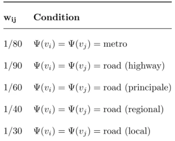
there exists an interconnection between them. The weight of each link is defined as the inverse of average speed that one could have over the corresponding edge. Table 2 represents the weight according to average speed over the edges of graph G. Wij =
wij if vi, vj are adjacent in G 0 otherwise.
(7)
2) Edge length: involving edge length in the transition probability, indirectly considers higher probability for the nodes close to each than that for farther ones. The transition probability between two intersections vi and vj is defined as the
wij Condition 1/80 Ψ(vi) = Ψ(vj) = metro 1/90 Ψ(vi) = Ψ(vj) = road (highway) 1/60 Ψ(vi) = Ψ(vj) = road (principale) 1/40 Ψ(vi) = Ψ(vj) = road (regional) 1/30 Ψ(vi) = Ψ(vj) = road (local)
Table 2: Edge classification and weights for multilayer transportation network G.
inverse of the shortest path cost between vi and vj:
T r(vi, vj) = ∑ ∀ (mn) ∈ SP vivj wmn× d(vm, vn) −1 (8)
where (mn) is an edge between vm and vn belonging to SPvivj, the shortest
path between two nodes vi and vj in graph G. The shortest path cost of SPvivj
is the sum of distances over each edge (mn) belonging to SPvivj, weighted by
wmn. d(vm, vn) is the euclidean distance between each two nodes vm and vn.
In earlier studies, the transition probability was quantified based on topo-logical properties of the underlying network which was mainly a road graph. In [19, 23], the transportation network was represented as road segments and transitions were assumed to occur between adjacent road segments. The au-thors in [23, 24] considered equal transition probabilities between nodes in the same road segment or nodes between road segments which are adjacent with an intersection. The transition probability in [17] is defined based on the Manhat-tan disManhat-tance between the grid cells of the road network. The objective of our proposed transition probability model is to minimize the bias of the mapping algorithm for layers with different topological properties.
4.2. Emission Probability
In HMM, at each time step t, there exists an observation ot which in our
study is characterized as ct =< lon, lat, rmaxt >t. The emission score reflects
the notion that it is more likely that a particular observation point is observed from a nearby intersection than an intersection farther away [23]. For studies in which GPS data were used as observations [23, 19, 18], the emission probability score is modeled by a normal distribution that is a function of the euclidean dis-tance between the observation point and the hidden state, and with a standard deviation estimated from sensor errors.
In this work, cellular antenna locations serve as observations; since there is no labeled data available to estimate cellular sensor errors, we build the Voronoi tessellation of cellular antennas in the area of study. In the voronoi network of cellular antennas, each cellular antenna Ci is characterized by radius riwhich is the maximum distance of the cellular antenna from the corresponding voronoi cell vertices. Our emission score is defined as a decreasing function of the distance between the antenna location and the hidden node (intersection):
P r(ot|vj)∝ 1.0 if : dtj ≤ rtmax ( rmax t dtj )β if : rmaxt ≤ dtj ≤ τ 0 otherwise. (9)
where dtj = d(ot, vj) is the euclidean distance between ot and intersection vj,
and τ is a threshold corresponding to the maximum distance that a cell phone can be hit by a cellular antenna. τ enforces the constraint that only intersections in the radius of τ from the cellular antenna could be considered as candidate states (nodes).
5. Evaluation
5.1. Dataset for Evaluation
In order to evaluate the proposed algorithm, GPS data are used as ground truth. We collected the cellular trajectories of 10 volunteer participants during
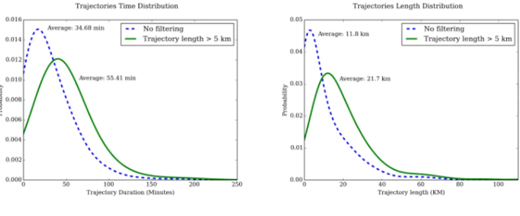
(a) Trajectory Time Distribution (b) Trajectory length Distribution Figure 6: Time distribution and distance distribution
one month (Aug-Sept 2014) with their corresponding GPS data. The GPS data were collected with the help of the application ”Moves” [28] which was installed on participants’ smartphones. The data captured were the sampled phone positions during its movements as well as its activities classified in four different categories: ’Walking’, ’Running’, ’Cycling’ and ’Transport’. Based on this dataset, a set of prepossessing steps were performed in order to extract trajectories mapped over the transport networks.
Furthermore, trajectories whose lengths are shorter than 5 kilometers were filtered out from the database. Given the low sampling rate of cellular data (a data point every 15 minutes), it is not realistic to seek recovering a movement that lasts less than this threshold. The effect of that filter on the dataset distribution could be observed in Fig. 6a and Fig. 6b.
The spatial accuracy needed in order to distinguish a real mobility from noise depends on the distance between two base stations. In order to filter out irrelevant movements, we filtered out all the trajectories under the threshold xth
such that Pr(X < xth) = q were Pr(X) is the distribution of distance between
neighboring antennas, for q = 0.97 as Fig. 7 shows all the neighboring distance is less than 5 kilometers.
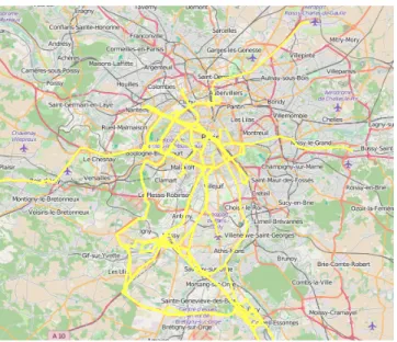
As conclusion, we built a dataset of 80 cellular trajectories (sequence of base stations) with their corresponding GPS paths mapped over a multilayer graph G. The multilayer transportation network contains around 16000 nodes and 26000 edges. The users trajectories covered a total distance of 2200 kilometers. The average number of observation points in each cellular trajectory is 5.55 and the average length of a trajectory is 26.5 kilometers. Fig. 8 shows the coverage area of collected the GPS trajectory dataset.
5.2. Evaluation Results and Comparison
5.2.1. Mapping algorithm efficiency
To evaluate our algorithm, the aforementioned labeled dataset was used for test and evaluation. We preformed CT-Mapper to map the cellular trajectories
Figure 8: The coverage area of GPS data collected is shown in yellow on the map of Paris and region
and to compare the result with GPS ground truth. Different measurements have been used to assess the performance of the Algorithm. First, we aim to quantify the similarity between obtained path and the ground truth. Since the algorithm infers the real trajectory in two phases, accordingly the result of the mapping algorithm in both two phases have been evaluated. This similarity is quantified using the Edit distance score, and one main reason is that this measure let us to compare two different sequences with different lengths by allowing different edits (deletion, insertion and substitution). We evaluate the two phases of the algorithm by calculating the edit-based similarity scores for both the skeleton and the complete mapped sequence. To have a comprehensive insight, we also calculate the average recall and precision of the results for dataset trajectories. Considering each trajectory as a set of nodes, precision is the fraction of re-trieved nodes that belong to the real path. Recall (also known as sensitivity) is the fraction of correct nodes that are retrieved by the algorithm. Moreover, in the evaluation section Root Mean Square Error (RMSE) have been used for two purposes: First, to quantify the overall distance between the obtained result and the ground truth. Second, owing to the considerable spatial noise of cellular ob-servations, RMSE is used to detect matches between 2 points using threshold ϵ . In this case, if the RMS error between two points is smaller than ϵ , we consider the inferred point as a match. For example, an error of 0.1 kilometers indicates that for each node in the output sequence, the node is considered as a match point if it is within a 0.1 kilometer radius of its corresponding real location. We calculated the four mentioned accuracy results (precision, recall, skeleton and complete sequence similarity score) for a range of fixed allowed RMSE on the ob-tained mapping results. The similarity scores are the complementary of the Edit distance scores. Fig. 9 represents the result of this evaluation. As Fig. 9 shows, with allowed RMSE of 200 meters, more than 50% of skeleton and complete trajectories can be retrieved. This is remarkable given the sparsity of the coarse grain cellular antenna positions with respect to real user trajectory (average of 5.5 observations per trajectory in the dataset while the average length is 26.5
col-lection is 15 minutes and with higher frequency, higher performance is expected for CT-Mapper. The average similarity score, for a RMSE of 1 kilometer, raises to 80%. In addition, CT-Mapper reaches a recall and a precision of around 80% when a RMSE of 1 kilometer is allowed. In addition to the metrics mentioned above, we compute the Edit distance error not as the number of required ed-its, but by considering the euclidean distance as the cost of each required edit. The average of Edit distances for all trajectories in the dataset is 0.79 kilometer.
5.2.2. Comparison with Baseline Algorithms
In this section, the performance of our proposed model is compared with two baseline models. Baseline 1 is a simple model that snaps each observation to the nearest node in the network to find the skeleton and for the second phase, uses least-cost paths between them to retrieve the full path. The result of this baseline model is compare with CT-Mapper in Fig.10.
To evaluate our transition probability model based on transportation properties as presented in Eq.(8), we derive Baseline 2, an HMM based baseline model associated with the naive assumption consisting of setting equal probabilities for all outgoing transitions from each node (including self node transition). Un-der such a model, the transition probability between two nodes vi and vj is
represented as: T r(vi, vj) = ki∗ ∏ n∈Q kn −1 (10)
where Q = SPvivj−{vi, vj} and kiis the degree of vi. This naive assumption
considers all the multilayer network edges on equal footing irrespective of their layer transportation properties .
Using this transition probability model, we build an HMM in the same way as CT-Mapper was developed. We use this model as a baseline algorithm and run it on the test dataset to compare the results with CT-Mapper. We calculate all four performance measures for the baseline models. Fig. 10 compares the performances of the two models with CT-Mapper. As the figures show, there
Figure 10: Up-left: Precision, up-right: Recall, bottom-left is Edit-based similarity scores and bottom-left is the skeleton similarity score
is up to 20% improvement in recall using our proposed transition probability model. Also the average Edit distance of the baseline algorithm result was 1.04 kilometer which proves that CT-Mapper performs significantly better compared to the second baseline algorithm. Fig. 11 shows the distribution of Edit distance for both the second baseline algorithm and CT-Mapper.
5.2.3. Multimodality analysis
In the next step of assessing our mapping algorithm, we investigate the accu-racy of the mapping algorithm in transportation layer detection. As mentioned in Sec. 8, the complexity of multimodal mapping significantly increases ow-ing to the considerable topological differences between transportation layers. This issue is dealt with in the proposed transition probability model that seeks minimizing the bias in the mapping algorithm.
Figure 11: Sequence Edist Distance
layer. The overall recall and precision for the whole network is computed as the average of recall and precision for each layer, weighted by the number of nodes. Fig. 12 shows these measures compared with the baseline algorithm. We have to notice that since each assumption considers specific aspect of network’s topological properties, they might introduce a bias in the mapping problem. As it is shown in Fig. 12, the overall recall and precision of correct layer detection is improved in CT-Mapper compared to the baseline algorithm.
6. Discussion & Conclusion
In this study, we proposed an unsupervised mapping algorithm (CT-Mapper) to map sparse cellular trajectories over a multimodal transportation network. We modeled and built the multilayer transportation network of subway, train and road layers for the Ile-de-France metropolitan area. The multilayer trans-portation network contains around 16000 nodes and 26000 edges. Investigating the complexity of the multilayer transportation graph, a transition probability model leveraging the transportation layer type and topological properties was estimated and used in an unsupervised HMM-based mapping algorithm. We carried experiments on a test dataset of 80 real multimodal trajectories col-lected from 10 participants during one month (Aug-Sept 2014) to evaluate our algorithm. Considering the sparsity of cellular observations (with a frequency of 15 minutes), the percentage of retrieved paths of smartphone users is no-table. To validate our transition probability model that better accommodates the complexity of the multimodal transportation network, we compared it with a baseline algorithm that does not take into account the transportation prop-erties of each layer and the results show up to 20% of accuracy improvement of the first over the second. We expect that using a dynamic weight matrix which is compatible with the traffic model at different times of the day, is likely to enhance the mapping results. This issue will be investigated in future studies. The improvement of accuracy measures of our mapping algorithm by minimizing bias mainly emanating from the multimodality of the transportation network is
of great importance which shall be discussed in future contributions. Investigat-ing the possibility of usInvestigat-ing the proposed mappInvestigat-ing algorithm at near real-time (NRT) for traffic monitoring is another direction of further contributions.
Ethics requirements and legal requirements followed during the data collection
Before starting the experiment of collecting cellular data we submitted the experiment protocol to the university ethics committee. Once the experiment started each volunteer signed a legal agreement stipulating that each of them requested access to their cellular localization data for one month (with a sam-pling interval of 15 min). This request was bond with a legal agreement given us the right to use their data for research purpose only. After one month of retention period after the end of the experiment, the cellular data were directly provided to the volunteers by the telecom operator. They forwarded us their cellular data afterward as well as their GPS traces.
Acknowledgment
This research received funding from the Pierre and Marie Curie University through their PhD founding program.
References
[1] S. Reddy, M. Mun, J. Burke, D. Estrin, M. Hansen, M. Srivastava, Using mobile phones to determine transportation modes, ACM Trans. Sen. Netw. 6 (2010) 13:1–13:27.
[2] J. Doyle, P. Hung, D. Kelly, S. McLoone, R. Farrell, Utilising mobile phone billing records for travel mode discovery, in: 22nd IET Irish Signals and Systems Conference, ISSC, 2011.
[3] Z. Smoreda, A.-M. Olteanu-Raimond, T. Couronn´e, Spatiotemporal data from mobile phones for personal mobility assessment, Transport survey
methods: best practice for decision making. Emerald Group Publishing, London (2013).
[4] C. Kang, S. Sobolevsky, Y. Liu, C. Ratti, Exploring human move-ments in singapore: A comparative analysis based on mobile phone and taxicab usages, in: Proceedings of the 2nd ACM SIGKDD Interna-tional Workshop on Urban Computing, UrbComp ’13, 2013, pp. 1:1–1:8. doi:10.1145/2505821.2505826.
[5] F. Giannotti, M. Nanni, D. Pedreschi, F. Pinelli, C. Renso, S. Rinzivillo, R. Trasarti, Unveiling the complexity of human mobility by querying and mining massive trajectory data, The VLDB Journal 20 (2011) 695–719.
[6] Detecting mobility patterns in mobile phone data from the ivory coast, in: ”Data for Challenge D4D 2013”, 2013.
[7] R. Agarwal, V. Gauthier, M. Becker, T. Toukabrigunes, H. Afifi, Large scale model for information dissemination with device to device communication using call details records, Computer Communications 59 (2015) 1 – 11.
[8] Y.-A. de Montjoye, C. A. Hidalgo, M. Verleysen, V. D. Blondel, Unique in the crowd: The privacy bounds of human mobility, Sci. Rep. 3 (2013).
[9] L. Liu, Data Model and Algorithms for Multimodal Route Planning with Transportation Networks, Ph.D. thesis, Technical University of Munich (TUM), 2011.
[10] M. C. Gonz´alez, C. A. Hidalgo, A.-L. Barab´asi, Understanding individual human mobility patterns, Nature 453 (2008) 779–782.
[11] D. Brockmann, L. Hufnagel, T. Geisel, The scaling laws of human travel, Nature 439 (2006) 462–465.
[12] F. Simini, M. C. Gonz´alez, A. Maritan, A.-L. Barab´asi, A universal model for mobility and migration patterns, Nature 484 (2012) 96–100.
[13] F. Giannotti, M. Nanni, F. Pinelli, D. Pedreschi, Trajectory pattern min-ing, in: Proceedings of the 13th ACM SIGKDD International Conference on Knowledge Discovery and Data Mining, KDD ’07, 2007, pp. 330–339. doi:10.1145/1281192.1281230.
[14] B. C. Cs´aji, A. Browet, V. A. Traag, J.-C. Delvenne, E. Huens, P. Van Dooren, Z. Smoreda, V. D. Blondel, Exploring the mobility of mobile phone users, Physica A: Statistical Mechanics and its Applications 392 (2013) 1459–1473.
[15] J. Yuan, Y. Zheng, X. Xie, Discovering regions of different functions in a city using human mobility and pois, in: Proceedings of the 18th ACM SIGKDD International Conference on Knowledge Discovery and Data Min-ing, KDD ’12, 2012, pp. 186–194. doi:10.1145/2339530.2339561.
[16] A. Abadi, T. Rajabioun, P. Ioannou, Traffic flow prediction for road trans-portation networks with limited traffic data, Intelligent Transportation Systems, IEEE Transactions on 16 (2015) 653–662.
[17] A. Thiagarajan, L. Ravindranath, H. Balakrishnan, S. Madden, L. Girod, Accurate, low-energy trajectory mapping for mobile devices, in: Proceed-ings of the 8th USENIX Conference on Networked Systems Design and Implementation, NSDI’11, USENIX Association, 2011, pp. 267–280.
[18] C. Goh, J. Dauwels, N. Mitrovic, M. Asif, A. Oran, P. Jaillet, Online map-matching based on hidden markov model for real-time traffic sensing applications, in: Intelligent Transportation Systems (ITSC), 2012 15th International IEEE Conference on, 2012, pp. 776–781. doi:10.1109/ITSC. 2012.6338627.
[19] P. Newson, J. Krumm, Hidden markov map matching through noise and sparseness, in: Proceedings of the 17th ACM SIGSPATIAL Inter-national Conference on Advances in Geographic Information Systems, GIS ’09, ACM, New York, NY, USA, 2009, pp. 336–343. doi:10.1145/1653771. 1653818.
[20] C. Hu, W. Chen, Y. Chen, D. Liu, Adaptive kalman filtering for vehicle navigation, Journal of Global Positioning Systems 2 (2003) 42–47.
[21] H. Xu, H. Liu, C.-W. Tan, Y. Bao, Development and application of a kalman filter and gps error correction approach for improved map matching, Journal of Intelligent Transportation Systems 14 (2010) 27–36.
[22] T. Hunter, T. Moldovan, M. Zaharia, S. Merzgui, J. Ma, M. J. Franklin, P. Abbeel, A. M. Bayen, Scaling the mobile millennium system in the cloud, in: Proceedings of the 2nd ACM Symposium on Cloud Computing - SOCC ’11, 2011, pp. 1–8. doi:10.1145/2038916.2038944.
[23] A. Thiagarajan, L. Ravindranath, K. LaCurts, S. Madden, H. Balakrish-nan, S. Toledo, J. Eriksson, Vtrack: Accurate, energy-aware road traffic delay estimation using mobile phones, in: Proceedings of the 7th ACM Conference on Embedded Networked Sensor Systems, SenSys ’09, 2009, pp. 85–98. doi:10.1145/1644038.1644048.
[24] B. Hummel, Map matching for vehicle guidances, in: R. Billen, E. Joao, D. Forrest (Eds.), Dynamic and Mobile GIS: Investigating Changes in Space and Time, CRC Press, 2006.
[25] R. van Nes, Design of multimodal transport networks : a hierarchical ap-proach, Ph.D. thesis, Technical University of Delft (DUP), 2002.
[26] A. Aguiar, F. Nunes, M. Silva, P. Silva, D. Elias, Leveraging electronic ticketing to provide personalized navigation in a public transport network, Intelligent Transportation Systems, IEEE Transactions on 13 (2012) 213– 220.
[27] Q. Xu, A. Gerber, Z. M. Mao, J. Pang, Acculoc: Practical localization of performance measurements in 3g networks, in: Proceedings of the 9th International Conference on Mobile Systems, Applications, and Services, MobiSys ’11, ACM, 2011, pp. 183–196. doi:10.1145/1999995.2000013.
[28] Moves, https://www.moves-app.com/, 2015.
[29] Institut gographique national, http://www.ign.fr/, 2015.
[30] Openstreetmap project, http://www.OpenStreetMap.org/, 2015.
[31] K. Sneppen, A. Trusina, M. Rosvall, Hide-and-seek on complex networks, Europhysics Letters (EPL) 69 (2005) 853–859.
[32] M. Rosvall, A. Trusina, P. Minnhagen, K. Sneppen, Networks and cities: An information perspective, Phys. Rev. Lett. 94 (2005).