HAL Id: hal-00293562
https://hal.archives-ouvertes.fr/hal-00293562
Submitted on 5 Jul 2008
A Cost-Regular based Hybrid Column Generation
Approach
Sophie Demassey, Gilles Pesant, Louis-Martin Rousseau
To cite this version:
Sophie Demassey, Gilles Pesant, Louis-Martin Rousseau. A Cost-Regular based Hybrid Column Gen-eration Approach. Constraints, Springer Verlag, 2006, 11 (4), pp.315-333. �10.1007/s10601-006-9003-7�. �hal-00293562�
Sophie Demassey ([email protected])∗
LINA FRE CNRS 2729, ´Ecole des Mines de Nantes, FR-44307 Nantes Cedex 3, France
Gilles Pesant ([email protected])
Centre for Research on Transportation, Universit´e de Montr´eal, C.P. 6128, succ. Centre-ville, Montreal, H3C 3J7, Canada
Louis-Martin Rousseau ([email protected])
Centre for Research on Transportation, Universit´e de Montr´eal, C.P. 6128, succ. Centre-ville, Montreal, H3C 3J7, Canada
Abstract. Constraint Programming (CP) offers a rich modeling language of con-straints embedding efficient algorithms to handle complex and heterogeneous com-binatorial problems. To solve hard comcom-binatorial optimization problems using CP alone or hybrid CP-ILP decomposition methods, costs also have to be taken into account within the propagation process. Optimization constraints, with their cost-based filtering algorithms, aim to apply inference cost-based on optimality rather than feasibility. This paper introduces a new optimization constraint, cost-regular. Its filtering algorithm is based on the computation of shortest and longest paths in a layered directed graph. The support information is also used to guide the search for solutions. We believe this constraint to be particularly useful in modeling and solving Column Generation subproblems and evaluate its behaviour on complex Employee Timetabling Problems through a flexible CP-based column generation approach. Computational results on generated benchmark sets and on a complex real-world instance are given.
Keywords: optimization constraints, hybrid OR/CP methods, CP-based column generation, branch and price, employee timetabling
1. Introduction
Constraint Programming based column generation is a decomposition method that can model and solve very complex optimization problems. The general framework was first introduced in [15]. It has since been applied in areas such as airline crew scheduling [9, 23], vehicle routing [22], cutting-stock [10], and employee timetabling [16].
All these optimization problems may be decomposed in a natural way: They may be viewed as selecting a subset of individual patterns within a huge pool of possible and weighted patterns. The selected
∗ A preliminary version of this paper appeared as [7]. This research was supported
by the Mathematics of Information Technology and Complex Systems (MITACS) Internship program in association with Omega Optimisation Inc. (CA)
combination is the one with the lowest cost to fulfill some given global requirements. The selection problem can be formulated as an integer linear program with one column for each possible pattern and a corre-sponding integer variable representing the number of times the pattern should be selected. The design of the possible patterns is itself a hard constrained satisfaction problem and its solution set may be too large to be written out explicitly. Delayed column generation is then the only way to address such a formulation (see, for example, [5] for details on the approach). The LP-relaxation of the integer program, the master problem, is solved iteratively on a restricted set of columns. At each iteration, the pricing problem is to generate new entering columns, i.e. new possible patterns, which may improve the current solution of the master problem.
In this approach, the pattern design subproblem is then solved sev-eral times. Each time, it is preferable to compute sevsev-eral solutions at once to limit the number of iterations of the column generation process. Also, an optimization variant of the problem should be considered since the expected patterns (i.e. the most improving columns) are the ones with the most negative reduced costs in the master problem.
In routing, crew scheduling or employee timetabling applications, the rules defining the allowed individual patterns are often multiple and complex. Traditionally, they have been handled by dynamic program-ming techniques [8]. The use of a constraint programprogram-ming solver instead to tackle the pricing problem adds flexibility to the whole solution procedure. For its modeling abilities, CP is more suited as rules are often prone to change.
Hence, CP-based column generation is an easily adaptable solu-tion method: the problem decomposisolu-tion makes the pattern design subproblem independent from the global optimization process, leaving the CP component alone to handle variations within the definition of the patterns. The recent introduction of both ergonomic and effective optimization constraints in the CP component can have a great impact on the success of this approach to solve various large-size optimization problems.
In this paper, we address a general class of employee timetabling problems with a CP-based column generation approach. The pattern design subproblem is then to build legal schedules with lowest costs for the employees. Legal schedules are defined as time-indexed activity sequences complying with a number of ordering or cardinality rules. We present the new optimization constraint cost-regular enclosing both the cost and the feasibility specifications of a sequence. This constraint, alone or supported by some side constraints, permits to define efficient and flexible CP algorithms for such optimum-cost
se-quence design problems: Firstly, it models together and in a handy way various complex sequencing rules (all described by a single deter-ministic automaton) and cost structures. Secondly, it simultaneously filters on feasibility and optimality criteria, making use of an efficient propagation (and back-propagation from the cost) algorithm. Last, its underlying support information serves as a helpful cost-based guiding heuristic for the search process. The contributions of this paper thus lie in the extension of the regular constraint [18] to handle efficiently cost information and in the hybrid column generation model it allows to define.
The paper is organized as follows: the next section reviews the work on optimization constraints while Section 3 presents cost-regular. In Section 4 we present the Employee Timetabling Problem and describe how hybrid column generation based on cost-regular can be used to solve it. Finally, experimental results are presented in Section 5 on both generated instances and a real world problem.
2. Optimization Constraints
Before discussing optimization constraints, let us first define the fol-lowing notation. Let S be the set of feasible solutions of a satisfaction problem. An instance of an optimization variant of this problem, at least in the mono-objective case, is given by an objective function f defined on a superset of S and taking its values in a totally ordered set, say IR. The problem is to find the minimal value z∗ the function f
takes on S and an element v∗ in S where f takes this value: f (v∗) = z∗. In Constraint Programming, the optimization criterion is generally taken into account by adding to the initial satisfaction model a cost variable z with interval domain. Additional constraints, modeling con-dition z <= f (v)∀v ∈ S, link the cost variable to the decision variables X. Constraint programming optimization algorithms solve a succession of satisfaction problems. Each time a new best solution is found, the upper bound of z’s domain is reduced to match its value.
Optimization constraints, by merging both feasibility and optimiza-tion condioptimiza-tions, are more efficient. They aim to filter from the decision variable domains, values appearing in no solution v ∈ S or whose cost f (v) does not belong to the current domain of z. Hence, domain reductions are also propagated from the bounds of the cost variable to the decision variables.
Optimization constraints also reduce the domain of z by computing a good evaluation of its lower bound. Constraint propagation can then detect inconsistency on this variable in the same way a traditional OR
branch-and-bound method does. Moreover, since it is often preferable to guide the search towards regions which are likely to contain low cost solutions, optimization constraints may compute additional informa-tion that can act as good variable-value selecinforma-tion heuristics or as regret notions (such as an optimal solution to a relaxation of the original prob-lem). We refer to Focacci, Lodi and Milano [12] for a further discussion about optimization-oriented global constraints. Several contributions have been made to the domain of optimization constraints. In general, the cost of an instantiation of the decision variables is computed as the sum of the costs cij of each assignment Xi= j.
Existing contributions hold mainly on weighted assignment con-straints such as the weighted all-different constraint [4, 11, 24], the global-cardinality with costs constraint [21], the sum of weights of dis-tinct values [3]. Among the other contributions, note the ones on the shorter path constraint [15, 25] which bears some similarities with the cost-regular constraint presented thereafter.
The cost-based filtering algorithms consist of propagating deduc-tion rules [3] or applying OR soludeduc-tion techniques to the optimizadeduc-tion problem or to a relaxation. Notable works in this domain are based on linearization and reduced-cost considerations [11, 17, 12, 26] or on graph algorithms [15, 21]. Remark that it is possible to achieve gen-eralized arc-consistency in polynomial time for some constraints (for example, the weigthed all-different [21]) while for NP-hard problems only relaxed consistency can be envisaged (see [10, 25]). In fact, opti-mization constraints merely share for now, cost-based filtering of the decision variable domains and one side-bounding of the cost variable domain. Much of these constraints concentrate on computing a tight lower bound of the cost to minimize but do not provide an upper bound ([3, 21] are among the exceptions). One reason is that lower and upper bounding are not always dual problems. Also only some of these constraints (e.g. [4, 12]) return information about the relaxed optimal solution computed during filtering (ie. the solution corresponding to the lower bound). Such precomputed informations would yet be very useful to guide the search towards minimal solutions in a backtracking algorithm.
Note that cost-based filtering algorithms are also used in soft-con-straints [1, 19, 27], where we wish to minimize a violation measure captured by a violation variable.
3. Cost-Regular
As the cost-variant of regular [18], constraint cost-regular(X, Π, z, C) holds if the values taken by the sequence of finite domain variables X spell out a word belonging to the regular language associated to the de-terministic finite automaton Π, and if z, a bounded-domain continuous variable, is equal to the sum of the variable-value assignment costs given by cost matrix C.1 The filtering algorithm associated to this constraint
is based on the computation of paths in a directed weighted layered graph. We show in this section how, by maintaining shortest and longest paths, the filtering algorithm of cost-regular provides: pruning on the lower and the upper bounds of the cost variable’s domain; cost-based pruning on the decision variables’ domains; and information to guide the search for solutions.
3.1. The Filtering Algorithm
A regular constraint is specified using a deterministic finite automaton that describes the regular language to which the sequence must belong. That automaton is then unfolded into a layered directed graph where vertices of a layer correspond to states of the automaton and arcs represent variable-value pairs. This graph has the property that paths from the first layer to the last are in one-to-one correspondence with solutions of the constraint. The existence of a path through a given arc thus constitutes a support for the corresponding variable-value pair [18].
Instead of simply maintaining paths, the filtering algorithm for cost-regular must consider the length of these paths, defined as the sum of the costs
of individual arcs. Since an arc corresponds to a variable-value pair, its cost is given by cost matrix C. Supports do not come from just any path but rather from a path whose length falls within the domain of z. To check this efficiently, it is sufficient to compute and maintain shortest and longest paths from the first layer to every vertex and from every vertex to the last layer: if the shortest way to build a path through a given arc is larger than the upper limit of the interval for z, the arc cannot participate in a solution and can thus be removed; if the longest way to build a path through a given arc is smaller than the lower limit of that interval, the arc can again be removed. In this way, domain consistency is achieved for the variables of X. The domain of z can also be trimmed using the shortest and longest paths from the first to the last layer.
1
Note that we could refine the costs further by associating one to every combination of variable, value, and state of the automaton.
x1 x2 x3 x4 x5 N1 N2 N3 N4 N5 N6 2 3 4 5 6 7 1 1 2 3 4 5 6 7 1 2 3 4 5 6 7 1 2 3 4 5 6 7 1 2 3 4 5 6 7 1 2 3 4 5 6 7 0 −10 −2 −4 0 0 0 0 0 0 0 1 1 1 −6 −6 0 0 0 0 −3 −6 0 −3 −3 −3 2 2 2 2
Figure 1. The layered directed graph built for a cost-regular constraint on five variables. Arc labels represent costs.
Figure 1 gives a layered directed graph built for the constraint on five variables. There are six layers, N1 to N6, and vertices within a
layer correspond to states of the automaton. An arc joining a vertex of layer Ni to another of layer Ni+1represents a feasible value for variable
xi: the arc’s color stands for the value and its label, the cost. If, for
example, the domain of z is [−12, −1], the topmost arc between layers N4 and N5, among others, will be removed because the shortest path
through it has length 2. Similarly, the third arc from the top between layers N1 and N2 will be removed because the longest path through it
has length −14 and furthermore since it is the only arc of this color for x1, the corresponding value is removed from its domain. Suppose now
that the domain of z is ]−∞, 5]: that domain will be trimmed to [−14, 3] since the shortest and longest paths in that graph are respectively of length −14 and 3.
The time complexity for the initial computation of the shortest and longest paths is linear in the size of X and in the number of transi-tions appearing in the automaton, due to the special structure of the graph. Subsequently these paths are updated incrementally, with a time complexity which is linear in the number of changes to the graph. 3.2. Search Guiding Heuristic
The shortest and longest paths maintained by the filtering algorithm are two constraint solutions with, respectively, minimal and maximal costs. These internal informations of the cost-regular constraint pro-vide a direct and efficient value ordering heuristic. When solving by
branch-and-bound a minimization (resp. maximization) problem in-cluding a cost-regular constraint, it makes sense to visit first the region of the search space where such an optimal but partial or relaxed solution is located.
To reach the constraint solution with minimal cost for example, the heuristic selects for a variable Xt the value corresponding to the t-th
arc in the shortest path in the layered digraph. With the current data structure underlying the filtering algorithm, such a value is accessible in linear time by following the shortest path from layers 1 to t.
4. Employee Timetabling Problems
Employee Timetabling Problems (ETP) constitute a general class of combinatorial problems widely encountered in industries and service organizations. An ETP is the problem of designing employee schedules over a given time horizon in order to cover the estimated workforce requirements of the organization. The timetabling attempts to optimize some performance criteria such as to minimize the overall labor cost or, alternately, to maximize quality of service. See [13] and [14] for extensive review on the subject.
In this paper, we address a general form of ETP. The main as-sumptions are that the time horizon is discrete and that the costs are additive along this horizon. The proposed solution method is applied to timetabling problems where employees are interchangeable (i.e. they may be assigned to any legal schedule). However, the method can easily be adapted to problems within the non-anonymous, personalized ETP class [7].
The following terminology and notation is used hereafter. The plan-ning horizon (e.g. one day) is partitioned as a sequence of T consecutive elementary time periods t ∈ {1, . . . , T }. We denote by W the set of work activities to perform. The workforce requirements specify the minimal number rat of workers required to achieve work activity a ∈ W at
period t ∈ {1, . . . , T }. A cost cat is associated to the assignment of one
worker to activity a at period t. Regulations often constrain the specific periods during which an employee is not assigned any work activity. To model these different constraints, additional activities (such as break, lunch or rest) are considered. These activities are not subjected to costs nor requirements (for notational convenience, we still define and set to 0 a cost cat for each non-work activity a and each period t). Let A
denote the entire set of work and non-work activities. A schedule is an assignment s : [1..T ] −→ A where s(t) stands for the activity to perform at period t. Alternatively, schedule s can be expressed by a
binary matrix ∆s = (δs
at)a∈A,t∈[1..T ] where δats = 1 if s(t) = a and
δsat = 0 otherwise. Let S denote the set of legal schedules or shifts which satisfy all the regulation constraints. Usual objectives in ETP are the minimization of the overall cost or the maximization of employee satisfaction. These criteria can be formulated by considering the cost cs for the company of allocating schedule s to an employee. Such a cost can also represent the degree of dissatisfaction for an employee being assigned to schedule s. The objective is then to minimize the sum of the costs of the schedules assigned to each employee. In the latter, cs is computed as the sum of the costs of performing activity
s(t) at period t: cs =PT
t=1cs(t)t. In some ETP formulations, the cost
of the staff timetabling may include penalties due to overcoverage or undercoverage. For each activity a ∈ W and period t, let ˆcat and ˇcat be
the additional cost when the timetabling covers the workforce demand rat with, respectively, one more employee and one less employee.
At the core of timetabling problems are various regulation con-straints (e.g. restraining work duration to exactly 8 hours a day, impos-ing a 15 minute break between two different work activities, permittimpos-ing a variable lunch time, changing work places) which arise in real world instances. Their number and complexity quickly make the subproblem of generating one legal schedule quite challenging.
4.1. CP-Based Column Generation for Timetabling
ETP are often solved in two steps. The first step consists of designing the possible shifts according to the regulation constraints. The opti-mization criterion is considered next by selecting the optimal subset of shifts to assign to the employees. However in many cases, the whole set of possible shifts is too huge to be processed at once. A column generation approach offers a way to solve ETP without generating the entire set of shifts. Following the same natural decomposition, shift generation is handled as the pricing subproblem while the selection problem is set as the master linear program. One legal shift corresponds to one variable or column in the master program.
This section presents a generic CP-based column generation ap-proach for Employee Timetabling Problems. We consider here the anony-mous case of ETP with minimum workforce requirements and with general work rules. The approach applies also to the personalized case or if additional over- and under-coverage costs are specified (see [7]). Since these variants hold on the selection subproblem alone, they re-quire a slight modification of the master linear program but do not change the pricing problem. On the other hand, work rules intervene only for shift generation. Specific rules may then be added as new
constraints within the pricing subproblem without changing the overall procedure. Column generation ends as soon as reaching an optimal fractional solution of the master program. We discuss in Section 4.3 about ways of finalizing the search to get either feasible or optimal integer solutions.
4.2. LP model and Column Generation
The integer linear formulation (P ) of the considered ETP turns into a generalized set-covering problem [6] with non-binary variables:
min X s∈S csxs (1) s.t. X s∈S δatsxs ≥ rat ∀ a ∈ W, ∀ t ∈ {1, . . . , T }, (2) xs≥ 0 ∀ s ∈ S, (3) xs∈ ZZ ∀ s ∈ S. (4)
A non-negative integer variable xs is associated to each legal schedule
s ∈ S, standing for the number of employees assigned to schedule s. Constraints 2 ensure to cover the minimum requirements for each work activity, at each period. The objective 1 is to minimize the sum of the costs for any working employees.
Being indexed by S, the set of variables of this linear formulation has order of |A|T. It can then generally not be computed at once.
A way of getting around this, is to solve the LP-relaxation ( ¯P) of (P ) (obtained by dropping constraints (4)) with the delayed column-generation technique. Hence, only a subset of legal schedules in S is produced and considered in ( ¯P). At each iteration of the procedure, new schedules are generated and the corresponding variables are added to the master linear program, only if they may improve its current solution. Here, the pricing problem of generating entering columns is to compute legal schedules s ∈ S with negative reduced cost rcs. If this
problem has no solution then the current solution of ( ¯P) is optimal. Given dual values (λat)W×{1,...,T } associated to the cover constraints 2
of the master program ( ¯P) at the current iteration, the reduced cost rcs of a schedule s equals to:
T
X
t=1
where c′at is defined for all activity a ∈ A and for all period t ∈ {1, . . . , T }, as: c′at= ( cat− λat if a ∈ W 0 otherwise. (6)
4.3. Integer Solutions and Branch-and-Price
Column generation applies to the LP-relaxation of the original integer program. The fractional solution returned at the end of the proce-dure corresponds to the assignment of an optimal selection of shifts to fractions of employees. Its cost gives a lower bound of the optimal timetabling cost.
Rounding up the fractional optimal solution of ( ¯P) leads to a fea-sible solution of the ETP but its cost is likely far from the integer optimum. In the present application, (P ) may contain numerous cover constraints. Moreover, each cover constraint involves a large number (order of |A|T−1) of non-zero values x
s. The high density of the LP
matrix makes the increased cost of this heuristic solution not negligible. Another heuristic solution is given by solving at optimality the integer program (P ) on the sole restricted set of generated columns. However, set-covering remains an NP-hard problem. In our test cases, even with only one working activity and few columns, such integer pro-grams were mostly too dense to be solved by a basic branch-and-bound (at least by the default procedure of Ilog Cplex).
Branch-and-price [2] is then the only alternative to compute an optimal integer solution and to prove its optimality. At each node of the tree search, a branching decision is added to the master program and column generation is invoked again to generate “missing” shifts and to evaluate the node.
It is known that associating a branching strategy with column gen-eration is not straightforward. In the present case, the conventional branching strategy for generalized set-covering models (separation on the domains of the pattern variables xs) is mostly deficient: The search
tree is clearly unbalanced (decision xs ≤ k is much weaker than xs ≥
k+ 1). The efficiency of the procedure depends heavily on the order of selection of the variables. The model admits lots of symmetries and op-timal solutions since many legal schedules are strongly similar. Lastly, when branching on a decision xs∗ ≤ k, the pricing problem has to
be explicitly constrained not to generate schedule s∗ anymore. Indeed,
given µs∗ ≥ 0 a dual value of the branching constraint in the master
program, then the non-negativity of the reduced cost of the schedule rcs+ µs∗≥ 0 does not prevent rcs<0.
Robust branch-and-price procedures, where branching does not in-crease the complexity of the pricing subproblem, have been proposed for several related problems, such as the capacited vehicle routing problem or the bin packing problem. These procedures, based on reformulations of the master program as a flow model, consist of branching on ag-gregated sum of variables. Such a reformulation applies to the master program considered here:
min X s∈S csxs (7) s.t. X b∈W fabt ≥ rat ∀ a ∈ W, ∀ t ∈ {1, . . . , T }, (8) fabt =X s∈S δatsδsb(t+1)xs ∀ a, b ∈ W, ∀ t ∈ {1, . . . , T }, (9) xs≥ 0, xs∈ ZZ ∀ s ∈ S, (10) fabt ≥ 0, fabt ∈ ZZ ∀ a, b ∈ W, ∀ t ∈ {1, . . . , T }. (11) In this LP, flow variable ft
abidentifies the number of employees assigned
to activity a at period t and to activity b at period t + 1. Branching on flow variables leads effectively to a more robust and balanced branch-and-price. Nevertheless, the usual arguments proving the completeness of such a branching scheme cannot be invoked here because of the integrality of both variables (not binary) and demands (not unary). Indeed, it is easy to find cases where all flow variables f are integer but not variables x. Consider for example, T = 4 and four sched-ules (a1, a3, a1, a3), (a1, a3, a2, a3), (a2, a3, a1, a3), (a2, a3, a2, a3) each
assigned to exactly 0.5 employee.
Even if the completeness is not guaranteed, this latter branching scheme can advantageously be used on top of the search, then eventu-ally completed by branching on a remaining fractional x variable each time all f variables are integer.
4.4. Shift Scheduling: a General CP model
The pricing problem within the proposed approach can be referred to as a Shift Scheduling Problem. The solutions of this problem are schedules s : {1, . . . , T } −→ A satisfying to all the regulation constraints and whose reduced cost rcsat the current iteration of the column generation
procedure is negative.
4.4.1. Regulation Constraints
The regulation constraints occurring in ETP usually fall into one of the five following classes of constraints:
− Allowed/forbidden assignments: Only activities in At ⊆ A may
be performed at period t. Such constraint avoids, for example, to schedule lunch before 1 pm.
− Cardinality rules: They specify the minimal ˇµA′ and the maximal
ˆ
µA′ numbers of periods assigned to activities in A′⊆ A. They may
constrain, for example, the work duration or the allowed number of break periods.
− Stretch rules: They specify the minimal ˇλa and the maximal ˆλa
number of consecutive periods assigned to activity a ∈ A. They may constrain, for example, the lunch duration or the minimal duration of a work activity.
− Sequencing rules: They specify the allowed and forbidden activity changes. They may force, for example, a break period between two different work activities.
− Conditional rules: These are logical combinations of rules of the four preceding classes. For example: a lunch of 1 hour is required if the work duration is greater than 3 hours a day.
The Shift Scheduling Problem can be modeled as a Constraint Satis-faction Problem based on a sequence of T decision variables s1, s2, . . . , sT
with finite discrete domains D1, D2, . . . , DT, initialized to A. There is
an obvious one-to-one correspondence between complete instantiations of these variables and schedules by setting s(t) = st for all periods t.
Assignment st= a means that activity a is performed at period t.
According to the first rule class, each domain Dt may initially be
restricted to At. The rules of the other classes need to be modelled
as constraints whose support includes all the decision variables. Fortu-nately, several existing global constraints are dedicated to handle such rules. Hence, having an overall viewpoint on the problem, the constraint propagation within such global constraints is likely to be quite effective. For the cardinality rules, a global cardinality (gcc) constraint [20] can be used to constrain, for all the activities, their number of occur-rences in the schedule. For each activity a ∈ A, a domain variable σa
with domain [ˇµa; ˆµa] is added to the model.
gcc(< s1, . . . , sT >, < σa|a ∈ A >). (12)
This constraint holds if each value a ∈ A is taken by exactly σavariables
among s1, . . . , sT. All other cardinality rules on subset A′ of activities
an arithmetic constraint
σA′ == X
a∈A′
σa. (13)
Note that usually, an ETP contains few rules of that kind.
Stretch and sequencing rules may be handled together with one or several regular global constraints [18]. Indeed, such rules define sequences of values which can be taken by the sequence of variables (s1, s2, . . . , sT). It is generally straightforward to represent all these
allowed patterns by a deterministic finite automaton Π whose transi-tions are labeled by the values (examples are given in [18, 7] and in Section 5.2). Note that, since the complexity of the filtering algorithm of regular is dependent of both the number of variables and the size of the automaton, one may envisage sometimes to have recourse to conjunctions of regular, with small automata, in order to model all the stretch and sequencing rules. Nevertheless, pruning is more efficient if all the rules are handled by one constraint alone. Furthermore, the complexity of the algorithm remains linear in those sizes and is able to tackle large-size instances. In our experiments, we used then only one such constraint (see Section 5):
regular(< s1, . . . , sT >,Π). (14)
Conditional rules can be formulated as logical constraints (and, or, not) in the CP model. These side constraints are highly dependent of the context of application. We considered various and complex ones in our experiments (see Section 5). A particular attention should be given to these constraints since they may considerably complicate the solution procedure. Indeed generally, such constraints propagate poorly and it can be advantageous to fix them in the first branches of the search tree. 4.4.2. Optimization Criterion
The constraints given above constitute a reasonable framework for a CP formulation of the Shift Scheduling Problem. As we consider the pricing problem of the column generation approach, costs have to be incorporated in order to generate only legal schedules with reduced costs. According to (5) and the correspondence between schedules and complete instantiations of (s1, s2, . . . , sT), the relation to model is
(s1 = a1, s2= a2, . . . , sT = aT) =⇒ T
X
t=1
c′att<0.
This relation can be inefficiently modeled using T global constraints element. As discussed in Section 2, with such a formulation, cost
pruning could mainly occur only once the feasibility part of the problem is solved.
Our goal is to use the negative cost criterion to prune the solution space earlier during the search. To achieve this, we propose to replace in the model the regular constraint (14) by its cost variant:
cost-regular(< s1, . . . , sT >,Π, z, c′). (15)
with initial domain ] − ∞, 0[ for z. By pruning both the lower bound lb and the upper bound ub of the domain of z, this constraint ensures that, at any current state of the search, there exist possible (according to Π) instantiations of variables (s1, s2, . . . , sT) whose costPTt=1c′att is
equal to lb or ub. Hence, if the instantiation is complete, z is equal to its cost. Conversely, any instantiation of the decision variables to values in their current domain is ensured to have a cost between lb and ub.
In the column generation procedure, this model of the pricing prob-lem is solved with a backtracking algorithm. One solution corresponds to one entering column in the master program. In fact, we aim to gener-ate several solutions at once. In the backtracking algorithm, the search is run until the expected number of solutions is found. Furthermore, we aim to generate solutions with the most negative reduced costs. Considering an optimization criterion within the model in order to find such optimal solutions could be clearly time-consuming since the whole search tree should be considered (implicitly though) before deciding if a feasible solution found is optimal. It is known that, in column generation procedures, looking systematically for the minimal reduced cost solutions of the pricing problem is not necessarily beneficial (at least when pricing is a hard problem).
Hence, rather than adding to the model a minimization criterion on z, we keep solving the satisfaction model but we use the heuris-tic returned by cost-regular to drive the search (Section 3.2). This heuristic does not ensure that the first complete instantiation found by the backtracking algorithm is optimal. Nevertheless, the principle of the heuristic makes us expect to find near optimal solutions.
We have experimented this strategy on the benchmark instances presented in an earlier paper [7]. A quick comparison of the computa-tional results obtained leaves no doubt on the great efficiency of this strategy, as shown in Section 5.1.
5. Case study
To evaluate the effectiveness of the proposed framework, we present computational results on a set of generated ETPs as well as a real
world problem taken from the data of a large bank. We present here the problem details and discuss the results obtained on these instances. The whole algorithm was implemented in C++ on top of libraries Ilog Cplex 9.0 and Solver 6.0. Experiments were run on an Opteron 250 under Gnu/Linux 2.6 and g++ 3.3.
5.1. Generic Benchmark Data
We based our first experiments on the benchmark data sets described in [7]. Although these instances are randomly generated, the benchmarks are based on data and rules from a real-world timetabling problem as the demand curves where obtained from a retail store.
5.1.1. Problem Details
10 sets (ETPn)n=1,...,10 of 10 instances each are available, parameter
n indicating the number of work activities (|W | = n). The planning horizon is one day decomposed into periods of 15 minutes (T = 96), and the work rules need the definitions of three non-work activities:
A= W ∪ {p (break), o (rest), l (lunch)}
1. Some activities a ∈ Ft are not allowed to be performed at some
periods t.
2. s covers between 3 hours and 8 hours of work activities.
3. If s is worked for at least 6 hours, then it includes exactly two breaks and one lunch break of 1 hour. Else, it includes only 1 break and no lunch is envisaged.
4. If performed, the duration of an activity a ∈ W is at least 1 hour. 5. A break (or lunch) is necessary between two different work
activi-ties.
6. Rest shifts have to be assigned only at the beginning and at the end of the day.
7. Work activities must be inserted between breaks, lunch and rest stretches.
8. The maximum duration of a break is 15 minutes.
The first condition simply consists of removing the forbidden activ-ities Ft from the initial domain of each variable st: Dt= A \ Ft.
The next two regulation constraints need the definition of additional decision variables. They can then be modeled as explicit constraints as well as, implicitly, by restricting the initial domain of the variables. One way of modeling the second condition is to use one additional variable σa for each work activity a ∈ W , with domain {0, 1, . . . , 32}
and representing the number of periods assigned to activity a, as well as a variable σ with domain {12, . . . , 32}, standing for the total number of working periods. Variables σa and st may be linked by the gcc. In
the same manner, we define cardinality variables σp, σo and σl for the
non-working activities (break, rest and lunch, respectively). To model the third condition, the domains of σl and σp are initialized to {0, 4}
and {1, 2} respectively. We can also logically deduce from the whole set of conditions that any valid schedules contain a number of rest periods between 58 and 83. As redundant constraints, we can then reduce the initial domain of σo to {58, . . . , 83}.
The last five constraints can be modeled with the help of only one regular constraint. Indeed, the values permitted by these constraints together for the sequence of variables (s1, . . . , sT) can be described by
a single automaton Π. Figure 2 depicts such an automaton when W contains two activities a and b.
a p l a o o a a a a b b b b b p l b o a o l l l
Figure 2. An automaton for two work activities a and b. The leftmost circle represents the initial state and shaded circles correspond to accepting states.
Given automata Π, the shift scheduling problem described above can be formulated by the following Constraint Satisfaction Problem (CP ): gcc(< σa|a ∈ A >, < a ∈ A >, < s1, . . . , sT >) (16) σ == X a∈W σa (17) σ <24 ⇒ (σl == 0 ∧ σp == 1) (18) σ ≥ 24 ⇒ (σl == 4 ∧ σp == 2) (19) regular(< s1, . . . , sT >,Π) (20) st∈ A \ Ft, ∀t = 1, . . . , T (21) σa∈ {0, . . . , 32}, ∀a ∈ W, σ ∈ {12, 32} (22) σl ∈ {0, 4}, σp ∈ {1, 2}, σo ∈ {58, . . . , 83} (23) 5.1.2. Computational Results
Table I. Column generation algorithm results on the generated instances using information from cost-regular to guide the search.
Group nb ∆LB/U B #iter. #col. CPU in sec. av. (max) av. av. av. (max) CPav. ET P1 10 2.5% (6.9%) 19 889 0.4 (1.2) 0.02 ET P2 10 2.8% (9.2%) 48 2340 3.7 (28.0) 0.03 ET P3 10 2.3% (6.4%) 52 2550 2.0 (2.9) 0.03 ET P4 10 3.3% (6.1%) 103 5063 12.5 (90.5) 0.04 ET P5 10 5.1% (10.4%) 86 4288 6.2 (11.3) 0.04 ET P6 10 4.7% (11.1%) 130 6493 13.8 (31.3) 0.05 ET P7 10 6.1% (8.4%) 137 6839 18.4 (30.6) 0.06 ET P8 10 6.0% (8.6%) 155 7736 25.4 (41.8) 0.07 ET P9 10 7.3% (10.9%) 155 7741 25.9 (31.9) 0.07 ET P10 10 8.7% (11.7%) 179 8974 42.0 (44.5) 0.09
Table I provides details of the CP-based column generation algo-rithm execution on each problem set ETPn. The huge difference between
these results and the preliminary ones presented in [7] (and reported in table II) is entirely due to the search heuristic used within the CP backtracking algorithm. Indeed, no other changes were made nei-ther in the algorithm’s implementation nor in the execution phase. In the present experiments, we used the variable-value ordering heuristic based on cost-regular (Section 3.2), while in [7], the heuristic used
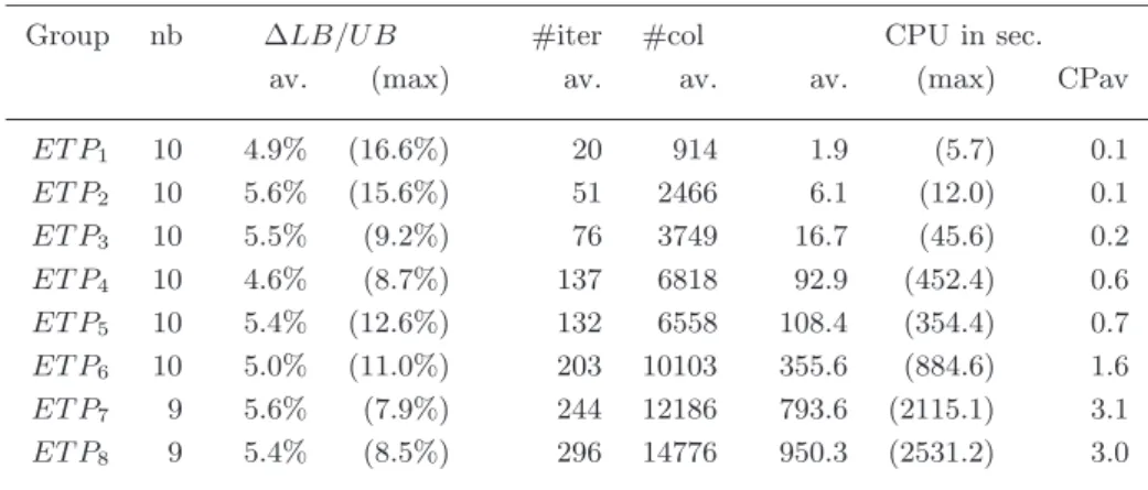
Table II. Column generation algorithm results on the generated instances using minimum reduced cost value to guide the search.
Group nb ∆LB/U B #iter #col CPU in sec. av. (max) av. av. av. (max) CPav
ET P1 10 4.9% (16.6%) 20 914 1.9 (5.7) 0.1 ET P2 10 5.6% (15.6%) 51 2466 6.1 (12.0) 0.1 ET P3 10 5.5% (9.2%) 76 3749 16.7 (45.6) 0.2 ET P4 10 4.6% (8.7%) 137 6818 92.9 (452.4) 0.6 ET P5 10 5.4% (12.6%) 132 6558 108.4 (354.4) 0.7 ET P6 10 5.0% (11.0%) 203 10103 355.6 (884.6) 1.6 ET P7 9 5.6% (7.9%) 244 12186 793.6 (2115.1) 3.1 ET P8 9 5.4% (8.5%) 296 14776 950.3 (2531.2) 3.0
was the minimal reduced cost first (instantiate first st∗= a∗ such that
(a∗, t∗) = arg min{ c′
at | (a, t) ∈ A × {1, . . . , T } }). The goal was indeed
to compute solutions with low cost.
Hence, the major difference within these results intervene in the computation time of the pricing subproblem solved by the CP back-tracking algorithm. In Tables I and II, column (CPav) gives for each set, the computation time of one pricing problem solution averaged over the number of iterations and the 10 instances. The average time is now lower than 0.1 second while it varied with the preceding heuristic from 0.1 to 3 seconds on average for the instances. In Table II none of the instances from group ET P9 and ET P10 were solved within the 1
hour time frame, we thus omitted these results.
In fact, with the former heuristic, CP backtracking was able to find 50 negative reduced cost solutions at almost every iteration (the CP search stopped after 5 seconds if it found at least one solution). But at the latest iterations, it was very slow to find the first (required) negative solution or to prove that none existed (it took up to 2500 seconds for ET P8 instances).
Choosing first the lowest cost assignments is indeed a clearly bad heuristic when no more negative solution exists. Conversely, the cost-regular based heuristic is effective at each iteration of the column genera-tion procedure: both when numerous negative solugenera-tions exist (in the first iterations), or to prove that no such solution exists (in the last iteration).
Another interesting conclusion coming from the comparison of these results is about the quality of the generated solutions. Indeed the
aver-age number of iterations (column (#iter.) in Table I) is lower with the new heuristic than with the former one in II. This has an impact on the number of columns required by the master program to reach the optimality (column (#col.) gives the average number on each instance set). This has also an impact on the total computation time (columns (CPU av.) et (CPU max.)).
Since the pricing problem returned about the same number of solu-tions, whatever the chosen heuristic (50 solutions an iteration, less in the very last iterations), the explanation of this difference is the higher quality of the solutions returned by the new heuristic.
The two first columns of Tables I and II give the average and maximum deviation of the lower bound LB computed by the column generation procedure (i.e the fractional optimum) to an upper bound U B. We computed U B by running the default branch-and-bound of Cplex on the sole generated columns. U B is the value of the best integer solution found after 1 hour. As previously said, the density of the LP-matrix makes difficult the IP processing. Even for instances in ET P1, where the average number of the IP variables is 889, the
Cplex branch-and-bound cannot complete the search in 1 hour except for two instances. For these 2 instances, the integrality gap is not closed (LB < U B). This indicates that either the lower bound is not tight or columns entering in an optimal integer solution are missing.
We ran the branch-and-price approach described in Section 4.3 on the instance sets. Nevertheless, in 2 hours, the method was only able to solve instances with less than 3 activities: 8 instances in ET P1 and
ET P2 and 4 instances in ET P3 (respectively in 144 seconds, 394
sec-onds, and 1592 secsec-onds, in average). These results lead to an interesting question since for these 20 instances, the branch-and-price proved in fact that the LB is also the integer optimum.
5.2. A Real-World Case
The approach was also evaluated on a real-life employee timetabling in-stance submitted by a Canadian bank. The local company’s subsidiary, considered here, consists of one central establishment, including front desk and back office, and 3 branches. In a same day, employees may be allocated to several places. Each of these 5 places is then viewed as a work activity. Rules are also defined on 4 non-work activities: rest, lunch, dinner and transfer (from a branch to the central desk).
The contractual regulations may differ for employees working full-time (35 hours a week) or part-full-time (between 20 and 30 hours a week). Since there is an additional cost for the company due to part-time workers, the timetabling must be set up on a weekly basis.
An estimation of the required number of employees is given on a 15 minutes basis for each activity. Overcoverage and undercoverage are allowed, but at least one employee must be present (mat = 1) at all
time but without exceeding the available space Mat).
The linear model (P ) has to be modified to take these additional costs into account but, since the new constraints (26) and (27) do not hold on the pattern variables xs, the pricing problem remains the same.
min X s∈S csxs+ X a∈W T X t=1 (ˆcatxˆat+ ˇcatxˇat) (24) s.t. X s∈S δsatxs+ ˇxat− ˆxat= rat ∀ a ∈ W, ∀ t ∈ [1..T ], (25) ˆ xat≤ Mat− rat ∀ a ∈ W, ∀ t ∈ [1..T ], (26) ˇ xat≤ rat− mat ∀ a ∈ W, ∀ t ∈ [1..T ], (27) xs∈ ZZ+ ∀ s ∈ S, (28) ˆ xat∈ ZZ+,xˇat ∈ ZZ+ ∀ a ∈ W, ∀ t ∈ [1..T ]. (29)
Note that the cost of a schedule s is no longer the sum of the costs of the activity-period assignments since it also depends on work duration: cs = PT
t=1cs(t)t + γs, where γs can take one of two distinct values
depending on whether s is a full-time work schedule or not.
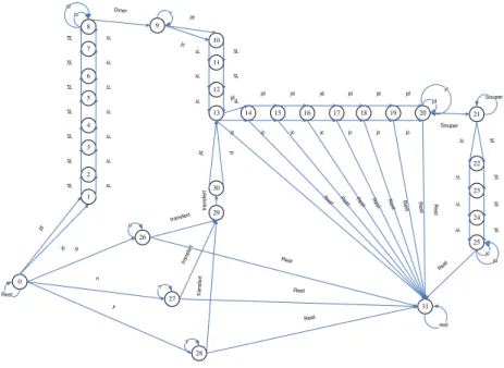
The work rules in this problem are quite complex. Allowed sequenc-ing and stretch patterns are given on a daily basis, but may be altered depending on the type of schedule. For example, lunch and dinner dura-tions differ for full-time and partial-time schedules. More complicated still: no employee may work after 5 pm more than one day in a week, and a part-time employee who works between 5 and 6 hours a day has to take a non-paid break of 15 minutes in the day. Another difficulty comes from the location considerations: a worker cannot do more than one transfer a day, and always from a branch to the center. In the center, no more than one activity change (between front desk and back office) is allowed per day. The automaton used to model this problem (shown in figure 3) gives an idea of difficulties presented by this application.
Furthermore, since we are constructing a weekly schedule, we need to introduce 5 cost-regular constraints in the model each modeling a day. This unfortunately reduces the effectiveness of the cost-regular constraint (both for filtering and guiding) but defining an automaton covering the whole week made the resolution intractable.
Since the column generation process does not converge in reason-able time, we need to interrupt it at some point in order to get a feasible solution to this complex instance. In this case however, Cplex is always able to solve the integer problem associated with the available
0 1 2 3 4 5 6 7 8 9 13 12 11 10 14 15 16 17 18 19 20 28 27 26 29 30 21 25 24 23 22 31 jd jc jd jc jd jc jd jc jd jc jd jc jd jc jd jc Diner jd jc jc jd jc jd jc jdjd jc jd jc jd jc jd jc jd jd jc jc jd jc jd Souper jc jc jd jc jd Rest jd jc p n y transfert tran sfe rt tr a nsfe rt tr a n s fe rt jc jd Rest Rest Rest Rest v Souper jc jd p n y jc jd Re st jc jd Res t R est R est R est Rest Res t R e s t rest
Figure 3. An automaton for the work and rest activities in a complex industrial timetabling problem.
columns very rapidly. The solutions obtained were comparable to those generated manually by the bank administration.
6. Conclusion
This paper presented a generic CP-based column-generation approach for Employee Timetabling Problems. In this approach, pricing is pro-cessed by solving a flexible CP formulation of the Minimal Cost Shift Scheduling Problem based on the new optimization constraint cost-regular. As other optimization constraints, cost-regular provides cost-based filtering of the decision variable domains as well as a tight lower bound of the problem. In a backtracking algorithm, the relaxed solution as-sociated to this lower bound gives effective and direct information to drive the search towards near optimal solutions. The filtering algorithm associated to cost-regular also computes an upper bound which acts as a heuristic value computed at each node of the search tree, and then improves the pruning of the search space. The design of opti-mization constraints is rather recent. Such constraints could be very
effective in solving optimization problems, if they provide together: cost-based filtering on the decision variables, filtering of both the lower and the upper bound of the cost variable domain, and the internal information computed by the filtering algorithm to be reused as search heuristic. Optimization constraints would be then entirely combinable, making the propagation more effective via the cost variable as it does on the decision variables, and improving search by selecting the most promising branching decision according to the heuristics returned by the constraints.
Acknowledgements
The authors wish to thank Alexandre le Bouthillier and Marc Brisson from Omega Optimisation Inc. for financial and technical support and also Andrea Lodi and Nicolas Beldiceanu for discussions and comments on parts of this paper.
References
1. Baptiste, P., Le Pape C., Peridy L.: Global Constraints for Partial CSPs: A Case-study of Resource and Due Date Constraints. Constraints (1998) 87–102 2. Barnhart, C., Johnson, L., Nemhauser, G., Savelsbergh, M., Vance, P.: Branch-and-Price: Column generation for solving huge integer programs. Operations Research 46 (1998) 316 – 329
3. Beldiceanu, N., Carlsson, M., Thiel, S.: Cost-filtering algorithms for the two sides of the Sum of the Weights of Distinct Values constraint. Technical Report SICS T2002:14 (2002)
4. Caseau, Y., Laburthe, F., Solving Various Weighted Matching Problems with Constraints. In Proc. 3rd Int. Conf. on Principles and Practice of Constraint Programming – CP’97, Springer-Verlag LNCS 1330 (1997) 17–31
5. Chv´atal, V.: Linear Programming. Freeman (1983)
6. Dantzig, G.: A comment on Edie’s traffic delays at toll booths. Operations Research 2 (1954) 339 – 341
7. Demassey, S., Pesant, G., Rousseau, L.-M.: Constraint programming based column generation for employee timetabling. In Proc. 2th Int. Conf. on Inte-gration of AI and OR techniques in Constraint Programming for Combinatorial Optimization Problems – CPAIOR’05, Springer-Verlag LNCS 3524 (2005) 140 – 154
8. Desrosiers, J., Dumas, Y., Solomon, M.M., Soumis, F.: Time constrained routing and scheduling. In M.O. Ball, T.L. Magnanti, C.L. Monna, and G.I. Nemhauser, editors, Network Routing, Handbooks in Operations Research and Management Science (1995) 35–139
9. Fahle, T., Junker, U., Karisch, S.E., Kohl, N., Vaaben, B., Sellmann, M.: Con-straint programming based column generation for crew assignment. Journal of Heuristics 8 (2002) 59–81
10. Fahle, T., Sellmann, M.: Cost based filtering for the constrained knapsack problem. Annals of Operations Research 115 (2002) 73–93
11. Focacci, F., Lodi, A., Milano, M.: Cost-Based Domain Filtering. In Proc. 5th Int. Conf. on Principles and Practice of Constraint Programming – CP’99, Springer-Verlag LNCS 1713 (1999) 189–203
12. Focacci, F., Lodi, A., Milano, M.: Optimization-Oriented Global Constraints. Constraints 7 (2002) 351–365
13. Ernst, A.T., Jiang, H., Krishnamoorthy, M., Owens, B., Sier, D.: An Annotated Bibliography of Personnel Scheduling and Rostering. Annals of Operations Research 127, (2004) 21-144
14. Ernst, A.T., Jiang, H., Krishnamoorthy, M., Sier, D.: Staff Scheduling and Rostering: A Review of Applications, Methods and Models. European Journal of Operational Research 153, (2004) 3-27
15. Junker, U., Karish, S.E., Kohl, N., Vaaben, N., Fahle, T., Sellmann, M.: A framework for constraint programming based column generation. In Proc. 5th Int. Conf. on Principles and Practice of Constraint Programming – CP’99, Springer-Verlag LNCS 1713 (1999) 261–274
16. Gendron, B., Lebbah, H., Pesant, G.: Improving the Cooperation Between the Master Problem and the Subproblem in Constraint Programming Based Column Generation. In Proc. 2th Int. Conf. on Integration of AI and OR tech-niques in Constraint Programming for Combinatorial Optimization Problems – CPAIOR’05, Springer-Verlag LNCS 3524 (2005) 217–227
17. Ottosson, G., Thorsteinsson, E.S.: Linear Relaxation and Reduced-Cost Based Propagation of Continuous Variable Subscripts. In Proc. Int. WS. on Inte-gration of AI and OR Techniques in Constraint Programming for Combina-torial Optimization Problems – CPAIOR’00, Paderborn Center for Parallel Computing, Technical Report tr-001-2000 (2000) 129 – 138
18. Pesant G.: A regular language membership constraint for finite sequences of variables. In Proc. 10th Int. Conf. on Principles and Practice of Constraint Programming – CP’04, Springer-Verlag LNCS 3258 (2004) 482–495
19. Petit, T., R´egin, J.-C., Bessi`ere, C.: Specific Filtering Algorithms for Over Constrained Problems. In Proc. 7th Int. Conf. on Principles and Practice of Constraint Programming – CP’01, Springer-Verlag LNCS (2001) 451–463 20. R´egin J.-C.: Generalized arc consistency for global cardinality constraints. In
Proc. of AAAI’96, AAAI Press/The MIT Press (1996) 209–215
21. R´egin J.-C.: Cost-based arc consistency for global cardinality constraints. Constraints 7 (2002) 387 – 405
22. Rousseau, L.-M., Gendreau, M., Pesant, G., Focacci, F.: Solving VRPTWs with constraint programming based column generation. Annals of Operations Research 130 (2004) 199–216
23. Sellmann, M., Zervoudakis, K., Stamatopoulos, P., Fahle, T.: Crew assignment via constraint programming: integrating column generation and heuristic tree search. Annals of Operations Research 115 (2002) 207–225
24. Sellmann, M.: An Arc-Consistency Algorithm for the Minimum Weight All Different Constraint. In Proc. 8th Int. Conf. on Principles and Practice of Constraint Programming – CP’02, Springer-Verlag LNCS 2470 (2002) 744–749 25. Sellmann, M.: Cost-Based Filtering for Shorter Path Constraints. In Proc. 9th Int. Conf. on Principles and Practice of Constraint Programming – CP’03, Springer-Verlag LNCS 2833 (2003) 694–708
26. Sellmann, M.: Theoretical Foundations of CP-based Lagrangian Relaxation. In Proc. 10th Int. Conf. on Principles and Practice of Constraint Programming – CP’04, Springer-Verlag LNCS 3258 (2004) 634–647
27. van Hoeve, W.-J., Pesant, G., Rousseau, L.-M.: On Global Warming: Flow Based Soft Constraints To appear in Journal of Heuristics (2005)