HAL Id: hal-02087289
https://hal.archives-ouvertes.fr/hal-02087289
Submitted on 5 Apr 2019HAL is a multi-disciplinary open access
archive for the deposit and dissemination of sci-entific research documents, whether they are pub-lished or not. The documents may come from teaching and research institutions in France or
L’archive ouverte pluridisciplinaire HAL, est destinée au dépôt et à la diffusion de documents scientifiques de niveau recherche, publiés ou non, émanant des établissements d’enseignement et de recherche français ou étrangers, des laboratoires
Probabilistic and sensitivity analysis of analytical models
of corrosion onset for reinforced concrete structures
Ndrianary Rakotovao Ravahatra, Emilio Bastidas-Arteaga, Franck Schoefs,
Thomas de Larrard, Frederic Duprat
To cite this version:
Ndrianary Rakotovao Ravahatra, Emilio Bastidas-Arteaga, Franck Schoefs, Thomas de Larrard, Fred-eric Duprat. Probabilistic and sensitivity analysis of analytical models of corrosion onset for reinforced concrete structures. European Journal of Environmental and Civil Engineering, Taylor & Francis, In press, �10.1080/19648189.2019.1591307�. �hal-02087289�
Probabilistic and sensitivity analysis of analytical models of corrosion onset for reinforced concrete structures
Ndrianary Rakotovao Ravahatraa,b, Emilio Bastidas-Arteagaa, Franck Schoefsa, Thomas de Larrardb, Fr´ed´eric Dupratb
aUniversit´e de Nantes, Research Institute in Civil and Mechanical Engineering (GeM), UMR
CNRS 6183, 2 rue de la Houssini`ere, BP 92208, 44322 Nantes cedex 3, France;bUniversit´e de
Toulouse, UPS, INSA, LMDC (Materials and Durability of Constructions Laboratory), 135 Avenue de Rangueil, F-31077 Toulouse Cedex 4, France
ARTICLE HISTORY Compiled March 4, 2019 ABSTRACT
Chloride ingress and carbonation are the main factors leading to corrosion initi-ation of reinforced concrete (RC) structures. Lifetime assessment and maintenance optimization of these deteriorating structures has been based for several practical applications on analytical predictive models. The literature review shows that there are numerous analytical models of chloride ingress and carbonation. It was also found that comprehensive lifetime assessment requires that the selected models be able to propagate uncertainties in a correct manner. Thus, this paper proposes a methodology for probabilistic sensitivity analysis of analytical models for chloride ingress and carbonation. Given that di↵erent parameter notations were found for each model, a homogenization of notations and generic forms are first proposed. The sensitivity analysis is based on the following indicators: elasticity coefficient, Pearson coefficient, bias of the mean and standard deviation of the response of the model. The results highlighted which parameters are influential for each model by considering three concrete types. Overall results indicated a higher e↵ect of the non-linearity of the models on the sensitivity indicators. It was found that the level of influence of each parameter depends also on the concrete type and the duration of the exposure to chlorides or carbon dioxide.
KEYWORDS
uncertainty, analytical models, sensitivity, carbonation, chloride ingress, reinforced concrete.
1. Introduction
Corrosion of steel reinforcement is a critical issue for many reinforced concrete (RC) structures; in particular, when they are located in chloride-contaminated environments and/or exposed to carbon dioxide (Tesfamariam et al., 2018). Given the high alkalinity of concrete after construction, a thin passive layer of corrosion products protects steel
Email: [email protected] Email: [email protected] Email: [email protected] Email: [email protected] Email: [email protected]
Please cite this article as:
Ndrianary Rakotovao Ravahatra, Emilio Bastidas-Arteaga, Franck Schoefs, Thomas de Larrard & Frédéric Duprat (2019): Probabilistic and sensitivity analysis of analytical models of corrosion onset for reinforced concrete structures, European Journal of Environmental and Civil Engineering, https://doi.org/
bars against corrosion, and therefore, the structure is initially protected from corrosion attack. Corrosion of rebars generally starts due to: (i) the breakdown of this protective oxide layer wrapping the rebar (chloride ingress), or (ii) the decrease of pH of the pore solution (carbonation).
The study of corrosion onset mechanisms in RC contributes to: (i) the better under-standing of the causes leading to corrosion, and (ii) the prevention or at least reduction of corrosion-induced damage (Winston Revie and Herbert H, 2008; Zhou et al., 2015). Both items are important for an optimal maintenance strategy based on inspection (condition assessment) and repair (damage mitigation). Nevertheless, in order to op-timize the resources allocated to the maintenance strategy and reduce environmental impact and failure risks, the prevention of corrosion-induced damage seems prefer-able (Bastidas-Arteaga and Schoefs, 2012, 2015; Li, 2003). Thus, an efficient detection and/or a realistic prediction of the corrosion initiation time can contribute to the reduction of maintenance costs and failure risks.
The present study is carried out within the framework of the ANR-EVADEOS project1. The main purpose of this project was to develop an engineering-oriented
approach for preventive maintenance optimization of RC structures exposed to corro-sion. It combines: non-destructive condition assessment, deterioration modeling, and inspection and maintenance optimization considering global uncertainties and allo-cated funds. Such an approach requires selecting degradation models with the following requirements:
(1) they should be able to account and propagate correctly the uncertainties involved in the problem (material properties, exposure, etc) (Rakotovao Ravahatra et al., 2017; Yajun and Xianming, 2012), and
(2) they should account for the availability of information and resources for param-eters estimation.
The selection of models that account for these requirements is still a challenge. We focus in this study on analytical models because they are used in engineering and some research applications. This paper will therefore provides to users useful informations when using these models with respect to the following considerations. First, it is dif-ficult to compare model outputs because models could use parameters obtained by di↵erent experimental tests whose accuracy are various (e.g., chloride di↵usion coeffi-cient estimated from migration test or chloride profiles). Second, although analytical models have a similar form, there is no a unified formulation of these models. Third, there is no comparison of the capacity of each model for propagating uncertainties for various materials and exposures. And fourth, the performance of each model when input information is more or less available is still unknown.
In this context, this paper aims at (i) providing unified formulations for chloride ingress and concrete carbonation models and (ii) perform a probabilistic sensitivity analysis to identify the more influencing parameters for each model.
The paper is organized as follows: section 2 provides an overview of models for corrosion onset assessment. Section 3 describes the summary and generalization of notations for several chloride ingress and carbonation models. Section 4 presents the studied material properties that were used in sections 5 and 6 for a sensitivity analysis based on four indicators: elasticity, Pearson coefficient, bias on the response mean, and standard-deviation of the response (Schoefs, 2008).
1Non-destructive evaluation of the structures for damage prediction and optimization of the follow-up.
2. Overview of corrosion onset models
The assessment of the corrosion initiation time of RC structures is based on chloride ingress or carbonation predictive models. Literature review shows two major groups of predictive models: analytical (or semi-analytical) and numerical. The first group of models is expressed by analytical or empirical equations. For chloride ingress, they are frequently expressed as a function of an error function (Collepardi et al., 1970; Euro-LightCon, 1999; JSCE, 2007; Petre-Lazar, 2001; DuraCrete, 2000; Tang and Gulikers, 2007). For carbonation, they are generally expressed in terms of a square root of time (CEB, 1997; Miragliotta, 2000; Papadakis et al., 1991; Petre-Lazar, 2001; DuraCrete, 2000; Ying-Yu and Qui-Dong, 1987). These analytical models were mainly developed for engineering purposes but they are still used for some research applications and require a reduced number of input parameters. However, the oversimplification of var-ious physical phenomena (e.g., some of them neglect the time-dependency of model parameters or correlation between parameters) could a↵ect the accuracy of their pre-dictions.
In contrast, numerical models account for various physical phenomena – e.g. the consideration of the e↵ects of heat and humidity transfers on chloride ingress or car-bonation processes. Therefore, they provide more informations on their outputs. They are generally expressed by partial di↵erential equations and require numerical meth-ods (finite elements, finite di↵erences, etc.) to be solved. Numerical models could lead to more accurate assessments of the corrosion initiation time; however, they require a larger number of model parameters (and experimental tests to characterize it) and vast end-user experience.
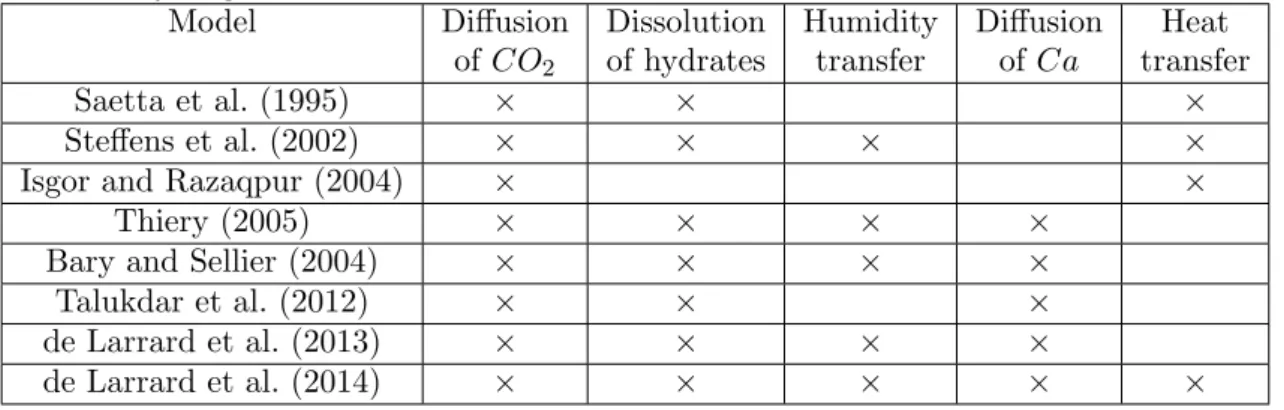
For Chloride ingress, we can find two major groups of numerical models: (i) those which are based on Fick’s law, that means without considering the interactions between chlorides and other ionic species (ii) those which depends on the law of Nernst-Planck, taking into account these interactions. We present in Table 1 and 2 the phenomena taken into account in some numerical models based on Fick’s and Nerns-Planck laws, respectively. For concrete carbonation, we present in Table 3 the phenomena taken into account in some numerical models.
Finally, the numerical model of Mai-Nhu (2013) takes into account simultaneously chloride ingress and concrete carbonation.
3. Summary of analytical models
3.1. Chloride ingress models 3.1.1. Unified formulation
Analytical models consider that chloride penetration through the porous network is mainly produced by the di↵erence in chloride content between the surface and the core of concrete. The phenomenon is described as a pure di↵usion process on a saturated concrete. These models also neglect the interaction between chlorides and other species in the pore solution. This simplifies the problem from ionic to molecular di↵usion. Analytical models of chloride ingress are then simplified solutions of Fick’s second law and could be expressed as a function of the complementary error function erfc or the Mejlbro-Poulsen function Mejlbro (1996). This work only considers unidimensional solutions based on the complementary error function because they are more used in
practice. The general form of these models takes the following generic expression: C(x, t) = Cserfc x 2p⇠(X, t) ! + Cini (1)
where C(x, t) is the chloride content [% wt. of concrete or % wt. of binder] at distance x from the concrete surface [m] and at time t [s], Cs is the chloride content at the
concrete surface that could be constant or time-dependent [% wt. of concrete or % wt. of binder], ⇠(X, t) is a general function of concrete di↵usivity which depends on a vector X of input parameters that are specific to each model and the time t [s]; depending on the models, concrete di↵usivity could be constant or time-dependent, Ciniis the initial chloride content of the concrete [% wt. of concrete or % wt. of binder].
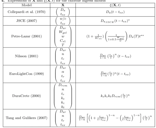
X and ⇠(X, t) are detailed in Table 4 for seven studied analytical models.
3.1.2. Model description and parameters
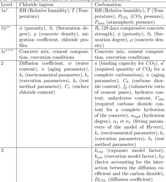
Figure 1 and Table 5 summarize the type of data required for each model. These input parameters can be classified into two levels. The parameters of level 1 can be provided directly by destructive or non-destructive testing or supplied in project archives (so-called “observables”). Any computation is necessary. The parameters of level 2 are deduced from level 1. The parameters of the second level are mostly used for chloride ingress modelling. This level includes material parameters (water content, apparent di↵usion coefficients, etc.) or factors derived to account for the kind of exposure, aging, etc. The evolution of chloride profiles (output) is obtained by evaluating the parameters of this level that correspond to the components of the vector X (eq. (1) and Table 4). Except one model that considers the e↵ect of temperature (Petre-Lazar, 2001), the parameters of the second level will be mostly considered in the sensitivity analysis.
Analytical chloride ingress models can be classified into two classes according to its capability to account for time-dependency of input parameters:
• Class 1: models without time-dependent input parameters (Collepardi et al., 1970; JSCE, 2007; Petre-Lazar, 2001).
• Class 2: models with time-dependent input parameters (EuroLightCon, 1999; DuraCrete, 2000; Tang and Gulikers, 2007).
3.1.3. Models without time-dependent input parameters
This category of models considers that all their input parameters are constant over time. Some of them account for uncertainties and the accuracy for determining their parameters, in a simplified way, through safety factors JSCE (2007). Other use empir-ical equations to account for interactions between ions or between chlorides and the concrete matrix Petre-Lazar (2001). Even if they are simpler, they are consistent with onsite discrete measurements in time, from which it is tricky to obtain time variant properties.
3.1.4. Models with time-dependent parameters
Various studies have shown that Dais time-dependent (Maage et al., 1995; Mangat and
Molloy, 1994; Sandberg, 1995; Takewaka and Mastumoto, 1998). Physically, concrete aging is due on the one hand to the micro-structure evolution caused by the continued
hydration of the cement and by carbonation. This causes a porosity reduction that slows down chlorides and CO2 penetration. On the other hand, during the di↵usion
process, the di↵erence between surface and bulk chloride contents is reduced along time till equilibrium. This implies that the gradient of chloride content decreases and thus also the kinetics of the di↵usion process. Other studies revealed or accounted for the time dependency of Cs (Bastidas-Arteaga et al., 2011; Crank, 1975; Swany et al.,
1995; Uji et al., 1990). The consideration of these time-dependencies could improve corrosion initiation assessment.
Concerning the time-dependency of the chloride di↵usion coefficient, three di↵usiv-ity definitions are found in the literature: instantaneous, average and achieved di↵u-sivity.
Instantaneous di↵usivity: is the value of the di↵usion coefficient at each time step. An expression deduced by rapid di↵usivity test is proposed in Tang and Nilsson (1992) as follows: D(t) = Dar ✓ tr t ◆n (2)
where Dar [m2/s] is the di↵usivity value determined at a reference time tr [s]. The
dimensionless parameter n is an age exponent. Eq. 2 should be integrated over time. However, some studies neglect this integration step for the assessment of di↵usion co-efficient (Maage and Molloy, 1995; Nilsson and Carcasses, 2004; Stanish and Thomas, 2003).
Average di↵usivity: is defined over the time interval [tex, t] (Frederiksen et al., 2008):
Dav(t) = 1 t tex Z t tex D(t) dt (3)
where tex is the age of the concrete at the beginning of the exposure to chloride
environment.
It can be expressed as follows:
Dav(t) = Dar ✓ tr t ◆ (4)
where Dar (m2/s) is the average di↵usivity at tr (s). The age exponent is not the
same as in eq. (2).
Tang and Gulikers (2007) gives the following expression, with the same age factor n as in equation (2). Dav(t) = Dar 1 n "✓ 1 + tex t tex ◆1 n ✓ tex t tex ◆1 n# ✓ tr t ◆n (5)
The DuraCrete model DuraCrete (2000) is supposed to use this di↵usivity definition with: Dav(t) = ktkckeDrcm ✓ tr t ◆n (6)
where kt, kc, ke, are respectively the test, cure condition and environmental
param-eters, Drcm is the migration coefficient obtained with rapid test according to
NT-Build492 (1999). Contradiction arose in the literature with respect to this statement about DuraCrete model. In Tang and Gulikers (2007) it is claimed that Dav(t) in eq
(6) is instantaneous di↵usion coefficient, since it is not underlined in the DuraCrete report DuraCrete (2000) that the compensation 1 n1 is introduced in ke or kc. Thus
an integration should be made over an interval in order to obtain the average dif-fusivity. In contrast, in Frederiksen et al. (2008), it is defined that Dav(t) in eq (6)
is the average di↵usivity. However, since the environmental parameter ke is obtained
without considering the time dependency of the surface chloride content (Cs), it is still
explained in Frederiksen et al. (2008) that this parameter is quantified erroneously. Given that the migration test duration t (s) is involved in the Drcm determination,
it is assumed in the present work that Drcm and therefore Dav(t) in eq (6) could be
considered as average di↵usivities.
Achieved di↵usivity: is the regression parameter Dach obtained by curve-fitting of
the following equation to a measured chloride profile (Nilsson, 1993):
C(x, t) = Cserfc x p Dach(t tex) ! + Cini (7)
Dach could be seen as the average di↵usivity in the time interval [tex, t] where t is
the age of the structure when the chloride profile is measured. Hence, a time dependent Dach(t) could be established using measurements at di↵erent time-steps.
The model proposed in the EuroLigthCon project (EuroLightCon, 1999) uses this di↵usivity definition. However, this model defines two age exponents: ↵ which corre-sponds to achieved di↵usion coefficient, and to the potential di↵usion coefficient ob-tained from a short time laboratory testing according to NTBuild492 (1999). The con-crete composition and environmental conditions are taken into account by ↵, whereas only concrete type is considered by . Therefore, the sensitivity analysis for this model will be only based on the parameter ↵. The reference EuroLightCon (1999) provides these parameters for some concrete types.
Concerning the time-dependency of surface chloride content, the false-erfc model (Nilsson, 2001), takes into account this e↵ect as:
Cs(t) = A ln(t tex) + B (8)
where A and B are fitting parameters.
Table 6 presents the input parameters for each studied chloride ingress model that are classified into environmental and material parameters.
3.2. Carbonation models 3.2.1. Unified formulation
Analytical carbonation models assume that carbon dioxide pressure varies linearly from the exposed surface, where it is equal to outer partial pressure, to the carbonation depth, where it is equal to zero due to the instantaneous CO2consumption by reaction
with dissolved hydrates. These models can be written in a generalized expression:
x(t) =pkexpkexekPDCO2
p
t (9)
where x(t) [m] is the carbonation depth at time t [s], kexp is a factor which introduces
environmental conditions, kexe is a factor accounting for execution conditions, kP is
a factor accounting for the interaction between the di↵usion coefficient of the carbon dioxide DCO2 [m2/s] and the concrete porosity . In some models (Hyvert, 2009;
Petre-Lazar, 2001; Ying-Yu and Qui-Dong, 1987), kP is expressed as:
kP = kP,MkP,E (10)
where kP,M is related to material properties and kP,E to exposure conditions.
Expres-sions of kP,M, kP,E, kexp and kexe are given in Table 7 for each considered model. ↵1
and n1 are fitting parameters, fp is the volumetric fraction of the cement paste, R
is the gas constant (8.31 USI), a is the binding capacity for CO2, a0 is the required
quantity of CO2 for a complete carbonation of the concrete studied, RH is relative
hu-midity, T is temperature, PCO2 is carbon dioxide pressure, Rc is concrete compressive
strength, is porosity, Sr is saturation degree, ⇢ is concrete density, [Component] is
the “component” content, Cabsis the absorbed carbone dioxide, C0is the CO2 content
at the exposed surface, ke is a parameter which assesses environmental conditions, kc
is a parameter which considers cure conditions.
The analytical models of carbonation can be divided into three classes:
• Class 1: models that mainly account for exposure conditions (Petre-Lazar, 2001; Ying-Yu and Qui-Dong, 1987).
• Class 2: models that mainly account for the potentially carbonated material content, estimated as a whole (CEB, 1997; DuraCrete, 2000) or as function of hydrates content (Miragliotta, 2000; Papadakis et al., 1991).
• Class 3: models that account for all previously mentioned factors (Hyvert, 2009). This study considers seven carbonations models (Table 7): two in class 1 (Petre-Lazar, 2001; Ying-Yu and Qui-Dong, 1987), four in class 2 (CEB, 1997; Miragliotta, 2000; Papadakis et al., 1991; DuraCrete, 2000), and one in class 3 (Hyvert, 2009). The following section presents the proposed classification of the parameters considered for all models.
3.2.2. Model description and parameters
In order to generalize the presentation of analytical models, the input parameters have been gathered into three levels (Figure 1 and Table 5). As well as for chloride ingress models, the parameters of level 1 are “observables”. Three kind of parameters could be found in the level 1:
• level 1a: environmental parameters – e.g. RH (relative humidity), T temperature; • level 1b: parameters which represent physical properties of concrete – e.g. Rc
(compressive strength), (porosity), Sr (saturation degree); and
• level 1c: other parameters – e.g. cement composition, concrete mixture, etc. The parameters of level 2 are deduced from level 1. The parameters of level 3 are derived from level 2 and they are the direct inputs of the models. The sensitivity analysis (section 4) will be carried out with respect to the parameters of levels 1
and 2 that are input parameters of models. The variability, according to hydrates or unhydrates contents, is quite difficult to supply and has been therefore introduced thoughtout the hydration degree ↵hyd and cement content c.
As well as for chloride ingress models, Table 8 presents the input parameters for each studied carbonation model that are classified into environmental and material parameters.
3.3. Discussion
It can be seen from Tables 6 and 8 that the number of input parameters varies from a model to another, from 3 to 10. It could be erroneously deduced that models requiring a larger number of parameters are the most accurate. Supplying models parameters is a more or less difficult task (in particular for the amount of hydrates in cement paste), and thus, may be a source of uncertainty and indirectly inaccuracy for lifetime assessment. Estimating the influence of uncertainties of parameters on the output of models is therefore an essential issue for probabilistic modeling. From building and infrastructure managers point of view, the choice of a model depends on both its accuracy and its cost in terms of informations to be supplied. When comparing the models according to their number of input parameters, it can only be stated that some of them are more elaborated than others. Sections 5 and 6 will study and compare the sensibility of these models to propagate uncertainties for the materials described in section 4.
4. Description of the studied materials
In order to represent various existing concrete structures, three typical concrete mixes have been accounted for: they are referred as C25, C35 and C45. These concretes were designed for specific earlier research works, except C35 concrete which was designed for the EVADEOS project. The compositions of CEM I cement and mixes of these concretes are reported in Table 9 and Table 10, respectively. Useful contents of hydrates in cement paste and concrete properties are reported in Table 11, where it can be noted that average resistances comply with European standard EN 206 (European Standard, 2004). Cement compositions are similar for all concretes and the variation of material parameters is mainly caused by the mix proportions (Table 9). For instance, incorporating three classes of aggregate size with an efficient balance between the respective amounts, led to a good compactness of the C45 concrete, with a favorable e↵ect on strength. But simultaneously the low water to cement ratio, w/c, prevented the content of hydrates to be high and the porosity remained rather elevated for the C45, despite the use of a superplasticizer. An almost opposite situation prevails for the C35 concrete, where both porosity and strength are rather low. Finally the C25 concrete is an ordinary quality concrete.
Outer surfaces of concrete structures considered in this study are supposed shel-tered and exposed to commonly encounshel-tered yearly average environmental conditions. Average relative humidity and temperature were thus 72% and 11 C, respectively.
5. Methodology and indicators for the sensitivity analysis
5.1. Notation and methodology
For the sensitivity analysis, analytical models of carbonation and chloride ingress are expressed as follows:
y = f (t, Z) (11)
where y is the model output, and Z ={z1, ..., zn} is the vector of input parameters of
the model.
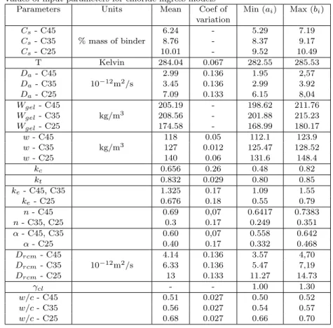
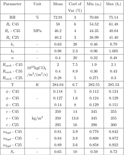
This study uses several sensitivity indicators: the elasticity coefficient, the Pearson’s coefficient, the bias on the mean, and the standard deviation of the response. The methodology follows the approach suggested in Schoefs (2008) for physical response surfaces. The values of input parameters are summarized in Tables 12 and 13 for chloride ingress models and carbonation models, respectively. The range of variability of each parameter corresponds to the possible realistic variability for the three studied concretes. The values of parameters that are considered as deterministic are presented in Table 14. Moreover, ke is determinated from DuraCrete (2000) as:
ke= 0 B @ 1 RH 100 2.5 1 ⇣RHref100 ⌘2.5 1 C A 5 (12)
where RHref corresponds to a reference relative humidity ('65%).
As previously mentioned, despite the fact that cement paste hydrates and unhy-drates contents are input parameters for some models, it was decided to consider their variability through hydration degree ↵hyd and cement content c, using the empirical
expressions, found in Hyvert (2009).
5.2. Elasticity coefficient
Elasticity measures the e↵ect on the output (here chloride content or carbonation depth) following a variation of one input parameter. The elasticity coefficient is com-puted deterministically as follows (Lemaire, 2009):
ei,k(t) =
yk(Z, t)(%)
zi(%)
at depth xk for chloride ingress models (13)
ei(t) =
y(Z, t)(%) zi(%)
for carbonation models (14)
where zi and y(Z, t) (or yk(Z, t)) are the variations of the input zi and the
model output, respectively. We considered an increase of 10% from the mean value for each input parameter. This value could be considered excessive or insignificant for some parameters; nevertheless, it is relevant to keep the same perturbation for all parameters. A larger absolute value of ei(t) means that the model is very sensitive
with respect to the variation of the considered parameter, while a value close to zero indicates a low sensitivity. A value of 1 means that a change of zi causes the same
5.3. Monte Carlo simulations for other sensitivity indicators
In order to analyse how the response of a system is influenced by the variation of its inputs, a common approach is to randomly vary these inputs into a given interval. Monte Carlo simulations are a relevant tool in such a purpose.
A variation interval [ai; bi] is defined for each input parameter (Tables 12 and 13),
whose bounds have been proposed from literature review (Buenfeld and Wong, 2009; GranDub´e, 2007; DuraCrete, 2000) or experimental data. Uniform distributions are used for generating random values.
5.3.1. Pearson’s correlation coefficient
Pearson’s coefficient ⇢corestimates the linear correlation between two random variables
(Bowley, 1901). In a sensitivity analysis of model parameters, the e↵ect of the ith
component zi of the input vector Z on y at the time t is assessed as follows:
⇢cor,xk(t) =
cov(yk(t), zi)
yk(t)⇥ zi
at depth xk for chloride ingress (15)
⇢cor(t) =
cov(y(t), zi)
y(t)⇥ zi
for carbonation (16)
where cov(yk(t), zi) (or cov(y(t), zi)) is the covariance between zi and y (or yk), and zi
and yk (or y) are their respective standard deviations. The value of ⇢cor varies from
-1 to 1. An absolute value close to 1 indicates a strong correlation while it indicates a low linear correlation when ⇢cor is approaching zero. A positive sign means a similar
trend of variation for both variables while a negative one indicates an opposite one. This indicator is able to highlight the physical meaning of the model and can also be used to rank input parameters according to their influences. However, Pearson’s coefficient is meaningful only if a linear or quasi-linear relationship between inputs and output is expected to exist.
5.3.2. Bias on the output mean value
This method is classified as a local method and relies on the OFAT (one-factor-at a time) method (Daniel, 1973). The previous sensitivity indicators aimed to evaluate the e↵ect of the variability of input parameters upon the model output in terms of proportionality (elasticity coefficient) and statistical dependency (correlation coeffi-cient). The global weight of a parameter can also be rendered by the bias imposed on the output mean value when it remains constant as the other parameters are ran-domly varying. This is assessed by the bias factor that is estimated using the following procedure (see Schoefs (2008)):
(1) compute, the global expected value E[f (t, Z)] of the output.
(2) fix the parameter zi at its mean value ¯zi; then, the ith component of the input
vector Z, now noted Zi0, is no longer random.
(3) estimate the bias factor regarding zi as:
bk,zi = E [yk(t, Z)] E [yk(t, Zi0)] at depth xk for chloride ingress (17)
5.3.3. Standard deviation of the output
This method is also one of the OFAT methods. The standard deviations of the car-bonation depth and chloride content at given depths are essential informations for estimating corrosion initiation risks. It is therefore of utter importance to examine how the standard deviation of the model output depends on the variability of input parameters. The procedure to estimate this indicator is summarized in the following steps (Schoefs, 2008):
(1) consider as random variable the parameter zi
(2) fix the other parameters at their mean values
(3) estimate The so-called reduced standard deviation of the output as:
zi/yk(t) =
r
Eh(yk(t, Zi) E [yk(t, Zi)])2
i
at depth xk for chloride (19)
zi/y(t) =
r
Eh(y(t, Zi) E [y(t, Zi)])2
i
for carbonation (20)
6. Results and discussions
6.1. Chloride ingress models 6.1.1. Elasticity results
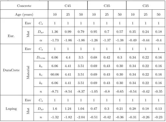
Tables 15 and 16 summarize the results obtained at 2.5 cm depth and 3 dates (10, 25 and 50 years) for first and second group of models, respectively.
Due to the linearity of all analytical chloride models with respect to Cs, the value
of elasticity is equal to 1 for all the models except for LEO model (Petre-Lazar, 2001). For this last one, the influence of the non-linearity decreases over time and the value of the elasticity tends to 1. The same trend is observed with respect to cl for the JSCE
model. On the other hand, when parameters are multiplying others in the model, the values of their elasticity are the same -e.g. ke, kc, kt and Drcm for the Duracrete
model (DuraCrete, 2000). Consequently, it is difficult to study the sensitivity of these parameters using this indicator.
Figure 2 illustrates the variation in time of the elasticity indicator for the Leo model, C25 concrete and x = 2.5 cm. As previously explained, analytical chloride ingress models describe an increase of the chloride content into the concrete bulk over time leading to a constant value which correspond to the chloride content on the concrete surface Cs. Consequently, at the beginning of the exposure to chloride environment,
the di↵usion process is significant and the di↵usion parameters such as Da, have higher
influence on the output of the model. For the same reason, similar results are found for di↵usion related parameters (e.g. Drcm and w/c ) in Tables 15 and 16. When the
chloride content into the concrete bulk is near to Cs, the di↵usion kinetic slows down.
At this stage, the only way that could boost up the process is a modification of the value of Cs. Any disturbance of the value of this parameter has significant impact
on the output of the model. The influence of di↵usion parameters is hence significant at the beginning of the exposure and decreases over time, while the influence of Cs
increases over time.
Concerning the aging parameter n (or ↵), one observe the same tendency as for di↵usion parameters: increasing influence at the beginning of the exposure and de-crease over time. Indeed, the kinetic of the aging of concrete (here, we are referring to continued hydration process, reduction of porosity caused by carbonation) slows down after long term exposure. The decrease starts earlier for material with lower resistance (C25 end C35).
The e↵ects of the type of concrete depend on the values and the variation range of the input parameters. When the concrete has higher resistance to chloride ingress (C45), material parameters have larger influence because any disturbance of the prop-erty of the involved concrete could a↵ect the kinetics of the chloride di↵usion.
6.1.2. Pearson’s coefficient results
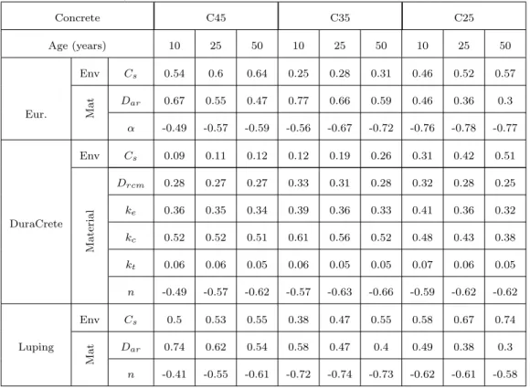
Tables 17 and 18 provide the Pearson’s coefficient results for the first and second group of models, respectively. Any conclusion could be made when the absolute value of this indicator is less than 0.5. Indeed, it may indicate either independence and/or non-linearity of the dependence. It is observed for all models a higher influence of di↵usion coefficients (Da, Dar) and kc. The temperature T has also large influence for the model
of Leo (Petre-Lazar, 2001). Finally, with respect to the models of the second group, the aging parameters n and ↵ have a significant impact. These results underline that aging of the concrete plays a significant role in the models of the second group.
Concerning the e↵ect of the concrete type, it was observed the same trend as for the elasticity coefficient.
6.1.3. Bias of the output
Tables 19 and 20 show the results for the first and second group of models, respectively. The non-linearity of the model with respect to the involved parameter increases the bias. Therefore, di↵usion and aging parameters (Da, Dar, kc, n and ↵) are the most
influential with respect to this indicator. However, lower values of bias are noted for Wgel, w, ke, kt, and Drcm because their variation ranges are smaller (Table 12).
Given that the output of analytical chloride ingress model has always positive value (chloride content), and that at the beginning of the exposure the values of the output are close to zero, the distribution of the output values is not symmetric. The values of the bias are hence positive during the first years of exposure for some model parame-ters, and then the sign changes. Figure 3 presents an illustration with the model of Leo and for concrete C25. For long-term prediction, the absolute values of bias decrease over time. Indeed, according to analytical chloride ingress model, the chloride content in the concrete bulk tends to Cs without exceeding this value. This means that the
mean model output tends to Cs, and thus the bias decreases.
Concerning the e↵ect of the type of material, when the concrete has higher resistance against chloride ingress, the kinetics of the phenomenon is lower. Consequently, the distribution of the output of the model remain asymmetric during a long period for this type of concrete (C45).
6.1.4. Standard deviation of the output
Tables 21 and 22 show the results with respect to output’s standard deviation for the first and second group of models, respectively.
The non-linearity of the model and the variation interval width of the input pa-rameters have significant impact on the standard deviation of the model output. This indicator provides better assessment of the ability of the models for uncertainty prop-agation. Indeed, it shows the variability on the model output when the parameter studied varies within its variation range. The parameters with respect to which the non-linearity of the model has significant impact for this indicator are Da, w, T , n and
↵. kc, kt and Drcmare multiplying factors in the model of Duracrete, their impact on
the model output depends on their variation ranges.
As well as for the bias, the standard deviation of the output of the model increases over time and decreases after a maximum, this with respect to di↵usion parameters such as Da, kc, ktand Drcm. The decrease begins when the di↵usion slows down which
is due to reduction of the gradient of chloride content. The decrease starts earlier for concretes with lower resistance against chloride ingress.
In the computation of this indicator, all the parameters are fixed to a predetermined value except the parameter of interest for the sensitivity analysis. The previous results were obtained considering the mean as the predetermined value, but they could di↵er for another selected value. It should be relevant to underline how the choice of another predetermined value of the fixed parameters would have an e↵ect on the results. Figure 4 presents an example with respect to the model of Collepardi and concrete C45. The input parameters of this model are Cs and Da. It is shown firstly in this figure,
the evolution of the output’s standard deviation when Cs varies and Da is fixed on
its minimum (CsminDa), mean (CsmeanDa) and maximum (CsmaxDa) values. And
secondly, the evolution of the output’s standard deviation when Da varies and Cs
is fixed at its minimum (DminCs), mean (DmeanCs)and maximum (DmaxCs) values.
No significant di↵erences could be observed concerning the ordering of parameters. It can be concluded from this figure that the order of importance is not a↵ected by the considered combinations.
6.2. Carbonation models
Table 23 summarizes the results of the sensitivity analysis for all carbonation models. For each model, the maximum and minimum value of each indicator are highlighted with bold text. The impact on the mean and standard deviation of the output varies over time, but the results of elasticity and the linear Pearson’s correlation coefficient remain fairly constant. Figures 5 and 6 present illustrations of the e↵ects of time with respect to elasticity and standard deviation respectively, for the model of Hyvert and for concrete C45. Since the order of importance of the parameters does not change over time, results are reported only for t=50 years which is the usual lifetime of RC structures.
6.2.1. Elasticity results
The non linearity of the models with respect to the parameter studied has significant impact on the value of its corresponding elasticity coefficient. For instance, elasticity coefficient are higher for the parameter n for the models CEB (CEB, 1997) and Du-racrete (DuraCrete, 2000), Rc for the Oxand model (Petre-Lazar, 2001), RH for the
models of Hyvert (Hyvert, 2009), Papadakis (Papadakis et al., 1991) and Miragliotta (Miragliotta, 2000). On the other hand, when parameters are multiplying other pa-rameters in the models, the values of their elasticity coefficient are similar e.g ke and
It was also found that time (t) has no e↵ect on the elasticity coefficient excepting models including the parameter n which is linked to t through the expression t0t n. However it has no e↵ect on the ranking of parameters.
Concerning the type of concrete, the material parameters (Rcarb, , c, ⇢, and ↵hyd)
have higher values of elasticity coefficient when the concrete has higher resistance against concrete carbonation. Indeed, from physical point of view, carbonation has lower kinetics in such concretes.
6.2.2. Pearson’s coefficient results
As well as for chloride ingress models, when the absolute value of this indicator is less than 0.5, any conclusion could be drawn. Results highlight the significant influence of the following parameters: RH, n, Rc, Sr, kc. No conclusion could be drawn with
respect to other parameters. As well as for the elasticity coefficient, time has no e↵ect on the Pearson’s coefficient. The e↵ects of the type of concrete are the same as for elasticity coefficient, -i.e., the coefficient of Pearson is higher for concretes with higher resistance against concrete carbonation.
6.2.3. Bias of the carbonation depth results
The values of the bias changed over time because carbonation models are increasing functions of time; however, the ranking of parameters for all models remained similar. The non-linearity of the model has significant impact on the bias. For instance, n is by far the parameter that introduces the higher value of bias for the models Duracrete (DuraCrete, 2000) and CEB (CEB, 1997). When the model has the same level of non-linearity with respect to two parameters, the one which has the larger width of variation interval has higher value of bias. For instance, parameter kc generates a
higher bias than ke and ktbecause it has a larger variation interval (Table 13).
In contrast to the previous indicators, the bias is small when the concrete has higher resistance against carbonation. Indeed, the kinetic of carbonation is reduced for the more resistant concretes, and therefore, the values of carbonation depth and its bias are smaller.
6.2.4. Standard deviation of the carbonation depth results
As well as for the bias, the standard deviation of the output of the model is very sensitive to non-linearity of the involved parameters. For example, large values were observed for parameter n with respect to which the models Duracrete (DuraCrete, 2000) and CEB (CEB, 1997) are significantly non-linear. It is possible to observe the same trend with respect to RH for the models of Oxand (Petre-Lazar, 2001), Miragliotta (Miragliotta, 2000), Papadakis (Papadakis et al., 1991), Ying-yu (Ying-Yu and Qui-Dong, 1987) and Hyvert (Hyvert, 2009). Similarly with respect to Sr for
the models of Miragliotta (Miragliotta, 2000) and Ying-Yu (Ying-Yu and Qui-Dong, 1987), and Rc for the model of Oxand (Petre-Lazar, 2001). The width of the variation
interval of the parameter has also significant impact. For instance, the parameters kc for the model Duracrete (DuraCrete, 2000), CEB (CEB, 1997) and the model of
Hyvert (Hyvert, 2009) have large variation interval width (Table 13).
Concerning the e↵ect of time, the standard deviation of the model output increases over time for any input variation. Figure 6 presents an example with the model of Hyvert and for the concrete C45. This means that a long-term prevision is a↵ected by more significant uncertainties.
Since the variation range of each parameter is not the same for each type of concrete (Table 13), the standard deviations of the model output are also di↵erent. Higher dispersion corresponds to concretes with lower resistance against carbonation (C35 and C25). On the other hand, for the Oxand model (Petre-Lazar, 2001), the order of parameters is not the same for two di↵erent materials because the gaps between the values of Rc are quite significant (Table 13).
As well as for chloride ingress models, it should be relevant to underline how the choice of another predetermined value of the fixed parameters would have an e↵ect on the results, especially for selected values leading to minimize or maximize the carbona-tion depth. For instance, regarding Oxand model (Petre-Lazar, 2001), minimum values of Rc and RH make easier the access of carbon dioxide into the concrete bulk. Figure
7 depicts the curves obtained for the combinations expected to modify the order of parameters with respect to the standard deviation for the Oxand model (Petre-Lazar, 2001). However, it can be observed in this figure that the order of importance is not a↵ected by the considered combinations.
7. Conclusions
Steel corrosion is one of the phenomenon that reduces significantly life-cycle of RC structures. This paper focused on analytical models of concrete carbonation and chlo-ride ingress that could be used to assess corrosion onset. An homogenization of these models leads to unified formulations. Two groups of models have been identified for chloride ingress models. The first one gathers models with constant parameters while the second one encompasses those with time-dependent parameters. For concrete car-bonation, three groups of models are highlighted. A classification of the input param-eters of these models has been proposed in which inputs are decomposed into three levels of parameters. This paper provided helpful tools for understanding and using these analytical models.
The relative importance of each parameter was assessed through the following indi-cators: elasticity coefficient, Pearson’s coefficient, bias, and standard-deviation of the output. In order to compute the three last indicators, the variation range of each input parameter for three concrete types are presented. It was found that the non-linearity of the models has significant impact in the values of each indicator as well as the variation range of the studied parameter.
The most influential parameters are Cs, Da and the aging parameters n or ↵ for
chloride ingress models. However, at earlier age, the di↵usion parameters have higher influence while at long-term, Cs becomes the most important parameter.
Concerning carbonation assessment the parameters which describe the porous media appear to be the most influential ones -i.e., RH which is linked to saturation degree, kc which gives an assessment of the quality of the firsts centimeters from the exposed
surface, and the porosity . Considering the variability of these parameters, it seems to be necessary to include it for a probabilistic assessment of carbonation. The second group of important parameters are those which introduced the amount of material that can be carbonated: the hydration degree ↵hyd and the cement content c.
These findings could help the end-user of a given model to optimally allocate the resources for obtaining each parameter. A parameter could be obtained either with expert advice or through destructive or non destructive tests. The amount of resources required to obtain a given parameter and then the required investment to use the cor-responding model depend on the methods used to obtain the parameters. Nevertheless,
the strategy of maintenance as well as the resources allocated are di↵erent for each structure. Within this framework, the results of this study could be used to develop a methodology for the choice of the appropriate model for a given structure, taking into account the chosen strategy of maintenance and the availability of the resources allocated to the maintenance. Rakotovao Ravahatra et al. (2019) present a framework to help decision-makers towards this aim.
Acknowledgements
This study has been carried out within the framework of the research project EvaDeOS (French National Research Agency - ANR 2011-VILD-002-01)
References
Baroghel-Bouny, V., Thi´ery, M., and Wang, X. (2011). “Modelling of isothermal coupled moisture-ion transport in cementitious materials.” Cement and Concrete Research, 41, 828– 841.
Bary, B. and Sellier, A. (2004). “Coupled moisture-carbon dioxide-calcium transfer model for carbonation of concrete.” Cement Concrete Research, (34), 1859–1872.
Bastidas-Arteaga, E. (2010). “Contribution for sustainable management of reinforced concrete structures subjected to chloride penetration.” Phd thesis, Universit´e de Nantes, Universit´e de Nantes.
Bastidas-Arteaga, E. (2018). “Reliability of Reinforced Concrete Structures Subjected to Corrosion-Fatigue and Climate Change.” International Journal of Concrete Structures and Materials, 12(1).
Bastidas-Arteaga, E., Chateauneuf, A., Sanchez-Silva, M., Bressolette, P., and Schoefs, F. (2011). “A comprehensive probabilistic model of chloride ingress in unsaturated concrete.” Engineering Structures, 33, 720–730.
Bastidas-Arteaga, E. and Schoefs, F. (2012). “Stochastic improvement of inspection and main-tenance of corroding reinforced concrete structures placed in unsaturated environments.” Engineering Structures, 41, 50–62.
Bastidas-Arteaga, E. and Schoefs, F. (2015). “Sustainable maintenance and repair of RC coastal structures.” Proceedings of the Institution of Civil Engineers - Maritime Engineering, 168(4), 162–173.
Bentz, E. and Thomas, M. (2008). Life-365 Service life prediction model. Bowley, A. (1901). Element of statistics. King and Son, Londres.
Buenfeld, N. and Wong, H. (2009). “Determining the watercement ratio, cement content, water content and degree of hydration of hardened cement paste: Method development and validation on paste samples.” Cement and Concrete Research, 39, 957–965.
CEB (1997). “New approach to durability design: an example for a carbonation induced corrosion.” Bulletin 238, CEB.
Collepardi, M., Marcialis, A., and Turriziani, R. (1970). “The kinetics of chloride ions pene-tration in concrete.” Il Cemento, 67, 157–164.
Crank, J. (1975). The mathmatics of di↵usion. Clarendon Press, Oxford, UK, second edition. Daniel, C. (1973). “One-at-a-time plans.” Journal of the American Statistical Association,
68(342), 353–360.
de Larrard, T., Bary, B., Adam, E., and Kloss, F. (2013). “Influence of aggregate shapes on drying and carbonation phenomena in 3D concrete numerical samples.” Computational Materials Science, 72, 1–14.
de Larrard, T., Bastidas-Arteaga, E., Duprat, F., and Schoefs, F. (2014). “E↵ects of climate variations and global warming on the durability of RC structures subjected to carbonation.” Civil Engineering and Environmental Systems, 31(2), 153–164.
Deby, F. (2008). “Approche probabiliste de la durabilit´e des b´etons en environnement marin.” Th`ese de g´enie civil, Universit´e de Toulouse Paul Sabatier, Universit´e de Toulouse III-Paul Sabatier.
EuroLightCon document BE96-3942/R3 (1999).
European Standard (2004). EN 206-1/A1 (April). ISSN 0335-3931.
Frederiksen, J., Mejlbro, L., and Nilsson, L.-O. (2008). “Fick’s 2nd law-complete solutions for chloride ingress into concrete.” Report no., Lund Institute of Technology, Lund University-Division of Buildings Materials.
Friedmann, H., Amiri, O., and A¨ıt-Mokhtar, A. (2012). “Modelling of edl e↵ect on chloride migration in cement-based materials.” Magazine of Concrete Research, 64(10), 909–917. GranDub´e (2007). “Grandeurs associ´ees la durabilit´e du b´eton.” Report no., Association
Fran¸caise du G´enie Civil.
Hyvert, N. (2009). “Application de l’approche probabiliste de la durabilit´e des produits pr´efabriqu´es en b´eton.” Phd thesis, Universit´e de Toulouse III-Paul Sabatier, Universit´e
de Toulouse III-Paul Sabatier.
Isgor, O. B. and Razaqpur, A. G. (2004). “Finite element modeling of coupled heat transfer, moisture transport and carbonation processes in concrete structures.” Cement and Concrete Composites, 26(1), 57–73.
JSCE (2007). “Proposed specification of durability design for concrete structures.” Report No. 15, Japan Society of Civil Engineers.
Lemaire, M. (2009). Structural Reliability. ISTE Ltd and John Wiley & Sons, Inc., Chapter Products of reliability analysis.
LERM, ed. (2000). Prediction of long-term durability of Vasco de Gama Bridge in Lisbon, Vol. 11, Barcelona, Spain. CANMET/ACI International conference.
Li, C. (2003). “Life cycle modeling of corrosion a↵ected concrete structuresinitiation.” Journal of Materials in Civil Engineering, 15(6).
Li, L. and Page, C. (2000). “Finite element modelling of chloride removal from concrete by an electrochemical method.” Corrosion science, 42, 2145–2165.
Maage, M., Poulsen, E., and Carlsen, J. (1995). “Service life model for concrete structures exposed to marine environment initiation period.” Report No. 2.4, LIGHTCON Report, Trondheim, Norway.
Maage, P. and Molloy, B. a. (1995). Practical non steady state chloride transport as a part of a model for predicting the initiation period, Vol. 2. RILEM, Chapter Chloride Penetration into Concrete, 398–406.
Mai-Nhu, J. (2013). “Corrosion des armatures du b´eton : couplage carbonatation/chlorures en pr´esence de cycles hydriques.” Ph.D. thesis, Universit´e Toulouse 3, Universit´e Toulouse 3.
Mangat, P. and Molloy, B. (1994). “Predicting of long term chloride concentration in concrete.” Materials and Structures, 27, 338–346.
Marchand, J. (2001). “Modeling the behaviour of unsaturated cement systems exposed to aggressive chemical environments.” Materials and structures, 34, 195–200.
Mejlbro, L. (1996). “The complete solution of fick’s second law of di↵usion with time dependent di↵usion coefficient and surface concentration, durability of concrete in saline environment.” Cementa AB, 127–158.
Miragliotta, R. (2000). “Mod´elisation des processus physico-chimiques de la carbonatation des b´etons pr´efabriqu´es - prise en comptes des e↵ets de paroi.” Ph.D. thesis, Universit´e de la Rochelle, Universit´e de la Rochelle.
Nguyen, P.-T., Bastidas-Arteaga, E., Amiri, O., and El Soueidy, C.-P. (2017). “An efficient chloride ingress model for long-term lifetime assessment of reinforced concrete structures un-der realistic climate and exposure conditions.” International Journal of Concrete Structures and Materials, 11(2), 199–213.
Nilsson, L. (2001). “Prediction models for chloride ingress and corrosion initiation in concrete structures.” Nordic Mini Seminar - Fib TD 5.5 Meeting, Goteborg.
Nilsson, L. and Carcasses, M. (2004). “Models for chloride ingress into concrete - A critical analysis.” Report no., EU-Project G6RD-CT-2002-00855,ChlorTest.
L.-O. Nilsson, ed. (1993). On a model of chloride ingress into concrete having time dependant di↵usion coefficient, Vol. P-93:1 of Chloride Penetration into Concrete, Gteborg. Nordic Mini Seminar, Poulsen, E.
Nilsson, L.-O., Sandberg, P., Poulsen, E., Tng, L., Andersen, A., and Frederiksen, J. (1997). “A system for estimation of chloride ingress into concrete, theoretical background.” Report no., HETEK.
NTBuild443 (1995). “Accelerated chloride penetration in hardened concrete. Nordtest. NTBuild492 (1999). “Concrete, mortar and cement based repair materials : chloride migration
coefficient from non steady state migration experiments. Nordtest.
Papadakis, V., Vayenas, C., and Fardis, M. (1991). “Fundamental modelling and experimental investigation of concrete carbonation.” ACI Materials Journal, 4(88), 363–373.
Petre-Lazar, I. (2001). “´evaluation du comportement en service des ouvrages en b´eton arm´e soumis `a la corrosion des aciers.” Ph.D. thesis, Universit´e Laval, Quebec.
Project BE95-1347, Final report (2000). DuraCrete Brite Euram III, eu edition.
Rakotovao Ravahatra, N., De Larrard, T., Duprat, F., Bastidas-Arteaga, E., and Schoefs, F. (Submitted in 2019). “A cost-benefit methodology for selecting analytical reinforced concrete corrosion onset models.” Advances in Civil Engineering.
Rakotovao Ravahatra, N., Schoefs, F., Duprat, F., de Larrard, T., and Bastidas-Arteaga, E. (2017). “Assessing the capability of analytical carbonation models to propagate uncertainties and spatial variability of reinforced concrete structures.” Frontiers in Built Environment: Bridge Engineering, 3(1), 1–9.
Saetta, A., Schrefler, B., and Vitalini, R. (1995). “2-d model for carbonation and moisture / heat flow in porous materials.” Cement and Concrete Research, 25(8), 1703–1712.
Sandberg, P. (1995). “Critical evaluation of factors a↵ecting chloride initiated reinforcement corrosion into concrete.” Report no., Lund institute of technologie, Buildings Materials. Schoefs, F. (2008). “Sensitivity approach for modelling the environmental loading of marine
structures through a matrix response surface.” Reliability Engineering and System Safety, 93, 1004–1017.
Sleiman, H., Amiri, O., and A¨ıt-Mokhtar, A. (2009). “Chloride transport in unsaturated cement-based materials: Modeling and simulation in case of a tidal zone.” European Journal of Environmental and Civil Engineering, 13(4), 489–499.
Stanish, K. and Thomas, M. (2003). “The use of bulk di↵usion tests to etablish tim-dependent concrete chloride di↵usion coefficients.” Cement and concrete research, 33, 55–62.
Ste↵ens, A., Dinkler, D., and Ahrens, H. (2002). “Modeling carbonation for corrosion risk prediction of concrete structures.” Cement and Concrete Research, 32(6), 935–941.
R. Swany, H. Hamada, T. Fukute, S. Tanikawa, and J. Laiw, eds. (1995). Chloride penetration into concrete incorporating mineral admixtures or protected with surface coating material under chloride environments, Saporo, Japan. CONSEC 95, E and FN, Spon and London, UK.
Takewaka, K. and Mastumoto, S. (1998). “Quality and cover thickness of concrete based on the estimation of chloride penetration in marine environments.” American Concrete Institute SP, 17(109), 381–400.
Talukdar, S., Banthia, N., and Grace, J. (2012). “Carbonation in concrete infrastructure in the context of global climate change: Part 1, experimental results and model development.” Cement and Concrete Composites, 34(8), 924–30.
Tang, L. and Gulikers, J. (2007). “On the mathematics of time-dependent apparent chloride di↵usion coefficient in concrete.” Cement and Concrete Research, 37, 589–595.
Tang, L. and Nilsson, L.-O. (1992). “Chloride di↵usivity in high strenght concrete at di↵erent ages.” Nordic Concrete Research, 11, 162–171.
Tesfamariam, S., Bastidas-Arteaga, E., and Lounis, Z. (2018). “Seismic Retrofit Screen-ing of ExistScreen-ing Highway Bridges With Consideration of Chloride-Induced Deterioration: A Bayesian Belief Network Model.” Frontiers in Built Environment, 4, 1–11.
Thiery, M. (2005). “Mod´elisation de la carbonatation atmosph´erique des mat´eriaux cimentaires - prise en compte des e↵ets cin´etiques et des modifications microstructurales et hydriques.” Ph.D. thesis, Ecole nationale des ponts et chauss´ees, Ecole nationale des ponts et chauss´ees. Uji, K., Matsuoka, Y., and Maruya, T. (1990). “Formulation of an equation for surface chloride
content of concrete due to permeation of chloride..” London: Elsevier Science, 26877. Winston Revie, R. and Herbert H, U. (2008). Corrosion and Corrosion Control-An
Introduc-tion to Corrosion Science and Engineering. A John Wiley & Sons, INC., 4th ediIntroduc-tion. Yajun, L. and Xianming, S. (2012). “Stochastic modeling of service life of concrete structures
in chloride-laden environments.” Journal of Materials in Civil Engineering, 24(4).
Ying-Yu, L. and Qui-Dong, W. (1987). “The mechanism of carbonation of mortars and the dependence of carbonation on pore structure.” ACI-SP 100, Concrete Durability, 1915–1943. Zhou, Y., Gencturk, B., Willam, K., and Attar, A. (2015). “Carbonation-induced and chloride-induced corrosion in reinforced concrete structures.” Journal of Materials in Civil Engineer-ing, 27(9).
Table 1. Physical phenomena that are taken into account in some numerical chloride ingress models based on Fick’s law
Model Di↵usion Humidity Heat
of chloride transfer transfer
LERM (2000) ⇥
Bentz and Thomas (2008) ⇥ ⇥
Deby (2008) ⇥
Clincon Nilsson et al. (1997) ⇥ ⇥
Bastidas-Arteaga (2010, 2018) ⇥ ⇥ ⇥
Nguyen et al. (2017) ⇥ ⇥ ⇥
Table 2. Physical phenomena that are taken into account in some numerical chloride ingress models based on the law of Nernst-Planck
Model Di↵usion Humidity Air
ionic species i transfer transfer
Clincon Nilsson et al. (1997) ⇥ ⇥
Li and Page (2000) ⇥
Marchand (2001) ⇥
Sleiman et al. (2009) ⇥ ⇥ ⇥
Baroghel-Bouny et al. (2011) ⇥ ⇥ ⇥
Friedmann et al. (2012) ⇥ ⇥ ⇥
Table 3. Physical phenomena that are taken into account in some numerical carbonation models
Model Di↵usion Dissolution Humidity Di↵usion Heat
of CO2 of hydrates transfer of Ca transfer
Saetta et al. (1995) ⇥ ⇥ ⇥
Ste↵ens et al. (2002) ⇥ ⇥ ⇥ ⇥
Isgor and Razaqpur (2004) ⇥ ⇥
Thiery (2005) ⇥ ⇥ ⇥ ⇥
Bary and Sellier (2004) ⇥ ⇥ ⇥ ⇥
Talukdar et al. (2012) ⇥ ⇥ ⇥
de Larrard et al. (2013) ⇥ ⇥ ⇥ ⇥
Table 4. Expressions of X and ⇠(X, t) for the chloride ingress models Model X ⇠(X, t) Collepardi et al. (1970) ✓ Da tex ◆ Da(t tex) JSCE (2007) ✓ w/c tex ◆ DaJSCE(t tex)⇤ Petre-Lazar (2001) 0 B B B B @ Dar Wgel w Cs1 T 1 C C C C A (1 + 1 4Cs1) 1 1+0.5Wgelw ! Da(T )t⇤⇤ Nilsson (2001) 0 B B @ Dar n tr tex 1 C C A D1 nar tr t n (t tex) EuroLightCon (1999) 0 B B @ Dar ↵ tr tex 1 C C A D1 ↵ar( tr t)↵(t tex) DuraCrete (2000) 0 B B B B B B @ Drcm n tr ke kc kt 1 C C C C C C A kekcktDrcm(ttr)n
Tang and Gulikers (2007) 0 B B @ Dar n tr tex 1 C C A 1 nDar ⇣ 1 + tex t tex ⌘1 n ⇣ t ex t tex ⌘1 n t r t n ⇤Da
JSCEis an empirical formula to determine Dain the model of JSCE for OPC: log10Da= 3.9(w/c)2+
7.2(w/c) 2.5
⇤⇤Da(T ) = Darexp⇣E
R(T1 2931 )
⌘
Table 5. Classification and data required for determining model input parameters
Level Chloride ingress Carbonation
1a⇤ RH (Relative humidity), T (Tem-perature)
RH (Relative humidity), T (Tem-perature), PCO2 (CO2 pressure),
Patm (atmospheric pressure)
1b⇤⇤ (porosity), Sr (Saturation
de-gree), ⇢ (concrete density), mi-gration coefficient, chloride pro-files
Rc(28 days compressive concrete
strength), (porosity), Sr
(Sat-uration degree), ⇢ (concrete den-sity)
1c⇤ ⇤ ⇤ Concrete mix, cement
composi-tion, execution conditions
Concrete mix, cement composi-tion, execution conditions 2 Di↵usion coefficient, w (water
content), n (aging parameter), ke(environmental parameter), kc
(execution parameters), kt (test
method parameter), Cs (surface
chloride content)
a (binding capacity for CO2), a0
(required quantity of CO2 for a
complete carbonation), n (aging parameter), C0 (carbone
diox-ide content), fp (volumetric ratio
of cement paste), hydrates con-tent, unhydrates concon-tent, Cabs
(required carbone dioxide con-tent for a complete hydration of the concrete), ↵hyd (hydration
degree), ↵1 et n1 (fitting
param-eters of the model of Hyvert), ke(environmental parameter), kc
(execution parameters), kt (test
method parameter)
3 kexp (exposure model factor),
kexe(execution model factor), kP
(factor accounting for the inter-action between the di↵usion co-efficient and the carbon dioxide), DCO2 (di↵usion coefficient)
⇤Meteorological data ⇤⇤Tests or project archives ⇤ ⇤ ⇤Project archives
Ta b le 6 . Input par ameter s of anal yti cal chl or ide ingr es s mo del s P ar am et er s Mo dels D es cr ip ti on S y m b ol C ol le p ar d i et al . (1970) JSC E (2007) P et re -Laz ar (2001) Ni ls son (2001) E u roLi gh tC on (1999) D u raC re te (2000) T an g an d G u li ke rs (2007) Env. C h lor id e con te n t on con cr et e su rf ac e Cs ⇥ ⇥ ⇥ Cs (t ) ⇤ ⇥ ⇥ ⇥ S af et y fac tor for Cs cl ⇥ T em p er at u re T ⇥ E n v ir on m en tal fac tor ke ⇥ Mat eri al W at er con te n t ! ⇥ G el con te n t W g el ⇥ Agi n g fac tor ↵ ⇥ n ⇥ ⇥ ⇥ Age at ex p os u re ti m e tex ⇥ ⇥ ⇥ ⇥ ⇥ Ref er en ce ti me tr ⇥ ⇥ ⇥ C u re con d it ion kc ⇥ F ac tor of te st m et h o d kt ⇥ R ap id ch lor id e m igr at ion co effi cien t Drc m ⇥ Ap p ar en t ch lor id e di ↵ u si on co effi cien t Da ⇥ Da JS C E ⇤⇤ Kno w n Da at re fe re n ce tim e tr Dar ⇥ ⇥ ⇥ ⇥ ⇤C s (t )= A ln( t tex )t + B , A and B are fitting parameters ⇤⇤ Empi ri cal for m ul a to deter mi ne Da in the mo del of JSCE for OP C: log 10 Da = 3 .9( w/ c) 2+7 .2( w/ c) 2 .5
Ta b le 7 . Expr es si ons of kP, E , kP, M , kex p and kex e Mo d el kP, E kP, M DCO 2 kex p kex e Yi n g -Y u a n d Qu i-D o n g (1 9 8 7 ) 2 PCO 2 / (C abs ⇢ ) 1 DYu =e x p (1 0 5 .66 0 .877) 1 1 Pa p a d a k is et a l. (1 9 9 1 ) C0 2 / ([ CH ]+3 [CS H ]+3 [C 3 S ]+2 [C 2 S ]) DPa =1 .64 ⇥ 10 6f 1 .8 p (1 RH) 2 .2 1 1 CEB (1997) C0 2 /a 0 DDu ( t0 t ) n ⇤ ke kc DuraCrete (2000) C0 2 /a kt DDu ( t0 t ) n ke kc Mi ra g li o tt a (2 0 0 0 ) C0 2(1 Sr )(1 ) 1([ CH ]+3 [CS H ]+3 [C 3 S ] D ⇤⇤ 1 1 +2[ C2 S ]+4 [C 4 AF ]+3 [C 3 A ]) 1 1 Pe tr e-L a za r (2 0 0 1 ) [ 3 .8533(RH ) 2 (365 ⇥ ( 1 2 .1 p R c ) 0 .06) 2 1 2 1 +3 .4833(RH ) + 0 .2] 2 1 Hyv er t (2 0 0 9 ) 2 PCO 2 R T f 1 p ⇣ [CH ]+4 [AF t]+3 [AF m ]+ 1 .65[ CS H ] n1 +1 ⇣ P CO 2 Patm ⌘n 1 ⌘ 1 D ke kc ⇥ ⇣ 1+ ↵1 1 .65[ CS H ] ⇣P CO 2 Patm ⌘n 1 ⌘ 1 ⇤D Du = a Rca r b ⇤⇤ D could b e measured through destructiv e testing or calcul a ted using prev ious empirical ex pressions, in this wo rk DPa is used
Ta b le 8 . Input par ameter s of anal yti cal mo del s of car b onati on Pa ra m et er Mo d el Description Sy m b ol Yi n g -Y u a n d Qui-Dong (1987) Pa p a d a k is et al. (1991) CEB (1997) DuraCrete (2000) Mi ra g li o tt a (2000) Pe tr e-L a za r (2001) Hyv er t (2 0 0 9 ) Env . CO 2 pressure PCO 2 ⇥ ⇥ Te m p er a tu re T ⇥ Rel ati v e h umi di ty RH ⇥ ⇥ ⇥ CO 2 con ten t C0 ⇥ ⇥ ⇥ ⇥ Mate ria l Po ro si ty ⇥ Saturation degree Sr ⇥ Compressiv e strength Rc ⇥ Ab so rb ed CO 2 Cabs ⇥ Concrete densit y ⇢ ⇥ Binding capacit y for CO 2 a ⇥ Requi red quan ti ty of CO 2 for ac o m p le tec a rb o n a ti o n a 0 ⇥ CS H con ten t [CS H ] ⇥ ⇥ ⇥ CH con ten t [CH ] ⇥ ⇥ ⇥ AF t con ten t [AF t] ⇥ ⇥ AF m con ten t [AF m ] ⇥ ⇥ C3 S con ten t [C 3 S ] ⇥ ⇥ C2 S con ten t [C 2 S ] ⇥ ⇥ C3 A con te n t [C 3 A ] ⇥ C4 AF con ten t [C 4 AF ] ⇥ ⇥ Refer ence p er io d t0 ⇥ ⇥ Fitting parameters ↵1 and n1 ⇥
Table 9. Cement composition (%)
Concrete SiO2 Al2O3 Fe2O3 CaO MgO SO3 K2O
C45 20.1 5 3 64.1 1 3.2 0.72
C35 20.43 4.9 1.83 65.4 1.06 3.5 0.25
Table 10. Concrete mixes
Concrete Cement Fly ash Sand Aggregates Aggregates Water Superpla- w/c
(kg/m3) (kg/m3) 0/4 4/12 12/20 (L/m3) sticizer
(kg/m3) (kg/m3) (kg/m3) (kg/m3)
C45 350 80 900 320 630 177 3 0.51
C35 350 0 815 998 0 195 1.4 0.56
Table 11. Physico-chemical properties
Concrete [AFm] [AFt] [CSH] [CH] SiO2 Porosity Rc
(mol/L) (mol/L) (mol/L) (mol/L) (mol/L) (%) (MPa)
C45 0.41 0.25 3.16 3.11 0 11.8 58
C35 0.41 0.15 3.185 3.585 0 12.7 46.2
Table 12. Values of input parameters for chloride ingress models
Parameters Units Mean Coef of Min (ai) Max (bi)
variation Cs- C45 6.24 - 5.29 7.19 Cs- C35 % mass of binder 8.76 - 8.37 9.17 Cs- C25 10.01 - 9.52 10.49 T Kelvin 284.04 0.067 282.55 285.53 Da- C45 2.99 0.136 1.95 2,57 Da- C35 10 12m2/s 3.45 0.136 2.99 3.92 Da- C25 7.09 0.133 6.15 8,04 Wgel- C45 205.19 - 198.62 211.76 Wgel- C35 kg/m3 208.56 - 201.88 215.23 Wgel- C25 174.58 - 168.99 180.17 w - C45 118 0.05 112.1 123.9 w - C35 kg/m3 127 0.012 125.47 128.52 w - C25 140 0.06 131.6 148.4 kc 0.656 0.26 0.48 0.82 kt 0.832 0.029 0.80 0.85 ke- C45, C35 1.325 0.17 1.09 1.55 ke- C25 0.676 0.18 0.55 0.79 n - C45 0.69 0,07 0.6417 0.7383 n - C35, C25 0.3 0.17 0.249 0.351 ↵ - C45, C35 0.60 0,07 0.558 0.642 ↵ - C25 0.40 0.17 0.332 0.468 Drcm- C45 4.14 0.136 3.57 4,70 Drcm- C35 10 12m2/s 6.33 0.136 5.47 7,19 Drcm- C25 13 0.133 11.27 14.73 cl - - 1.00 1.30 w/c - C45 0.51 0.027 0.50 0.52 w/c - C35 0.56 0.027 0.54 0.57 w/c - C25 0.68 0.027 0.66 0.70 NB : Means no data
Table 13. Values of input parameters for carbonation models
Parameter Unit Mean Coef of Min (ai) Max (bi)
Var (%) RH % 72.91 3 70.68 75.14 Rc C45 58 6 54.52 61.48 Rc - C35 MPa 46.2 4 44.35 48.04 Rc C25 40.2 3 38.99 41.40 kc - 0.63 26 0.46 0.79 kt - 0.98 2.3 0.96 1.005 n - 0.4 20 0.32 0.48 Rcarb - C45 1010kgCO2 /m3/(m2/s) 2 7.5 1.9 2.1 Rcarb - C35 0.4 8.9 0.36 0.43 Rcarb - C25 0.28 5 0.271 0.3 T K 284.04 6.7 282.55 285.53 - C45 0.118 5 0.112 0.124 - C35 - 0.127 1.6 0.124 0.129 - C25 0.14 8 0.129 0.151 c - C45 350 14 345 355 c - C35 kg/m3 350 13.6 345 355 c - C25 295 16 290 300 ↵hyd - C45 0.81 3.9 0.778 0.842 ↵hyd - C35 - 0.84 3.8 0.808 0.872 ↵hyd - C25 0.89 3.6 0.858 0.922 Sr - 0.65 10 0.59 0.72
Table 14. Deterministic parameters
Parameter Unit Value
Patm Pa 101325 PCO2 Pa 40.53 C0 kg/m3 6.5⇥10 4 - 1 ↵1 L/mol 23.5 n1 - 0.67
Table 15. Elasticity coefficient for the models of the first group of chloride ingress models (non time-dependent parameters) at 2.5 cm Concrete C45 C35 C25 Age (years) 10 25 50 10 25 50 10 25 50 Collepardi Env Cs 1 1 1 1 1 1 1 1 1 Mat Da 3.1 1.31 0.74 0.52 0.27 0.17 0.31 0.17 0.11 JSCE En v Cs 1 0.99 0.99 1 1 1 1 0.99 1 cl 1 1 1 1 1 1 1 0.99 1 Mat w/c 1.1 0.64 0.43 1.12 0.66 0.45 0.72 0.44 0.3 LEO En v Cs 0.68 0.86 0.92 0.97 0.98 0.99 0.98 0.99 0.99 T 646.32 51.5 17.27 6.1 2.8 1.69 4.45 2.15 1.33 Ma t Wgel -3.16 -1.5 -0.84 -0.38 -0.19 -0.12 -0.25 -0.13 -0.08 w 4.14 1.6 0.84 0.36 0.18 0.11 0.23 0.12 0.07 Da 11.11 3.77 1.9 0.84 0.42 0.26 0.64 0.32 0.2
Table 16. Elasticity coefficient for the models of the second group of chloride ingress models (with some time-dependent parameters) 2.5 cm Concrete C45 C35 C25 Age (years) 10 25 50 10 25 50 10 25 50 Eur. Env Cs 1 1 1 1 1 1 1 1 1 Ma t Dar 1.36 0.99 0.79 0.95 0.7 0.57 0.35 0.24 0.18 ↵ -1.73 -1.86 -1.86 -1.26 -1.37 -1.38 -0.49 -0.44 -0.4 DuraCrete Env Cs 1 1 1 1 1 1 1 1 1 Ma te ri a l Drcm 6.06 4.4 3.5 0.68 0.42 0.3 0.34 0.22 0.16 ke 6.06 4.41 3.51 0.69 0,43 0.30 0.34 0.22 0.16 kc 60.06 4.41 3.51 0.69 0.43 0.30 0.34 0.22 0.16 kt 6.06 4.41 3.51 0.69 0.43 0.30 0.34 0.22 0.16 n -8.71 -8.54 -8.37 -1.05 -0.8 -0.65 -0.54 -0.42 -0.35 Luping Env Cs 1 1 1 1 1 1 1 1 1 Ma t Dar 1.6 1.24 1.04 0.47 0.3 0.21 0.28 0.18 0.13 n -1.32 -1.82 -2.04 -0.51 -0.42 -0.36 -0.31 -0.26 -0.23
Table 17. Pearson’s coefficient for the models of the first group of chloride ingress models (non time-dependent parameters) at 2.5 cm Concrete C45 C35 C25 Age (years) 10 25 50 10 25 50 10 25 50 Collepardi Env Cs 0.35 0.63 0.81 0.98 0.99 0.99 0.71 0.87 0.94 Mat Da 0.93 0.78 0.59 0.16 0.08 0.05 0.69 0.46 0.32 JSCE En v Cs 0.84 0.85 0.85 0.42 0.43 0.43 0.47 0.47 0.47 cl 0.5 0.51 0.51 0.85 0.87 0.88 0.86 0.87 0.87 Mat w/c 0.104 0.08 0.05 0.26 0.15 0.1 0.17 0.11 0.08 LEO En v Cs 0.09 0.23 0.41 0.29 0.51 0.69 0.38 0.62 0.78 T 0.51 0.52 0.48 0.5 0.45 0.37 0.12 0.1 0.08 Ma t Wgel -0.09 -0.09 -0.08 -0.07 -0.06 -0.05 -0.05 -0.04 -0.03 w 0.14 0.14 0.13 0.02 0.02 0.02 0.12 0.1 0.08 Da 0.86 0.8 0.76 0.8 0.71 0.6 0.77 0.64 0.51
Table 18. Pearson’s coefficient for the models of the second group of chloride ingress models (with some time-dependent parameters) at 2.5 cm Concrete C45 C35 C25 Age (years) 10 25 50 10 25 50 10 25 50 Eur. Env Cs 0.54 0.6 0.64 0.25 0.28 0.31 0.46 0.52 0.57 Ma t Dar 0.67 0.55 0.47 0.77 0.66 0.59 0.46 0.36 0.3 ↵ -0.49 -0.57 -0.59 -0.56 -0.67 -0.72 -0.76 -0.78 -0.77 DuraCrete Env Cs 0.09 0.11 0.12 0.12 0.19 0.26 0.31 0.42 0.51 Ma te ri a l Drcm 0.28 0.27 0.27 0.33 0.31 0.28 0.32 0.28 0.25 ke 0.36 0.35 0.34 0.39 0.36 0.33 0.41 0.36 0.32 kc 0.52 0.52 0.51 0.61 0.56 0.52 0.48 0.43 0.38 kt 0.06 0.06 0.05 0.06 0.05 0.05 0.07 0.06 0.05 n -0.49 -0.57 -0.62 -0.57 -0.63 -0.66 -0.59 -0.62 -0.62 Luping Env Cs 0.5 0.53 0.55 0.38 0.47 0.55 0.58 0.67 0.74 Ma t Dar 0.74 0.62 0.54 0.58 0.47 0.4 0.49 0.38 0.3 n -0.41 -0.55 -0.61 -0.72 -0.74 -0.73 -0.62 -0.61 -0.58