Protein dynamics from accurate low-field site-specific longitudinal
and transverse nuclear spin relaxation
Pavel Kadeřávek,1,† Nicolas Bolik-Coulon,1 Samuel F. Cousin,1,‡ Thorsten Marquardsen,2 Jean-Max Tyburn,3 Jean-Nicolas Dumez,4 Fabien Ferrage1,*
1) Laboratoire des Biomolécules, LBM, Département de chimie ; École normale supérieure, PSL University, Sorbonne Université, CNRS ; 75005 Paris, France
2) Bruker BioSpin GmbH; Silberstreifen 4, 76287 Rheinstetten, Germany
3) Bruker BioSpin ; 34 rue de l’Industrie BP 10002, 67166 Wissembourg Cedex, France 4) CEISAM ; CNRS, Université de Nantes ; 44300 Nantes, France
† Present address: Central European Institute of Technology, Masaryk University, Kamenice 5, 625 00 Brno, Czech Republic
‡ Present address: Univ Lyon, CNRS, Université Claude Bernard Lyon 1, Ens de Lyon, France * Corresponding author email: [email protected]
This article is dedicated to the memory of Alfred G. Redfield (1929-2019).
Keywords: nuclear magnetic resonance • NMR relaxation • protein dynamics • high-field NMR spectroscopy • low-field NMR spectroscopy
Abstract: Nuclear magnetic relaxation provides invaluable quantitative site-specific information on the dynamics of complex systems. Determining dynamics on nanosecond timescales requires relaxation measurements at low magnetic fields, incompatible with high-resolution NMR. Here, we use a two-field NMR spectrometer to measure carbon-13 transverse and longitudinal relaxation rates at a field as low as 0.33 T (proton Larmor frequency 14 MHz) in specifically labeled sidechains of the protein ubiquitin. The use of radiofrequency pulses enhances the accuracy of measurements as compared to high-resolution relaxometry approaches, where the sample is moved in the stray field of the superconducting magnet. Importantly, we demonstrate that accurate measurements at a single low magnetic field provide enough information to characterize complex motions on low nanosecond timescales, which opens a new window for the determination of site-specific nanosecond motions in complex systems such as proteins.
Nuclear spin relaxation is a remarkable macroscopic phenomenon, which provides quantitative information about motional processes on the microscopic scale. High-resolution NMR measurements of relaxation result in the characterization of motions at the atomic scale and are extremely valuable to characterize the properties of a host of molecular systems.1,2 Relaxation
probes molecular motions at the characteristic frequencies of the spin system.3,4 Thus, relaxometry,
the measurement of relaxation rates over magnetic fields that span several orders of magnitudes (typically from ~100 µT to ~1 T), has provided invaluable information on motions over a broad range of timescales in polymers,5,6 biopolymers,7-10 water in porous media11,12 and solution of
paramagnetic molecules,13 including contrast agents.14-16 However, the low and rather
inhomogeneous magnetic field at which detection is performed in conventional relaxometry provides only low-resolution spectra, where all site-specific information is lost. To understand motional properties with atomic resolution, a radically different approach has been followed: high-resolution measurements of nuclear spin relaxation on high-field NMR spectrometers.17 In this
case, the density of motions is probed on the narrow range of frequencies (e.g. Larmor frequencies of nuclei) defined by the range of accessible high magnetic fields.18 However successful2,18 for
investigations of the protein backbone17,19 and side chains,20-24 as well as nucleic acids,25-27 this
limited sampling makes the interpretation of relaxation rates highly model-dependent.28,29 The
combination of high-resolution NMR and relaxometry has become recently possible with the use of sample shuttles on commercial high-field spectrometers.30-34 Such systems transfer the samples
to low-field positions in the stray field of a commercial magnet for relaxation while detecting signals in the magnetic center to benefit from high sensitivity and resolution. This approach permits the measurement of typically 10 to 30 relaxation rates covering about two orders of magnitude of magnetic fields, which has led to a series of successful studies of relaxation in small
molecules, proteins, nucleic acids or lipids 34-39, it suffers from a series of key limitations. First,
measurements at tens of magnetic fields are time-consuming. Second, the strong magnetic field gradients of the stray field prevent the measurements of relaxation rates of coherences. Third, measured longitudinal relaxation rates suffer from systematic deviations due to the absence of control of cross-relaxation pathways at low magnetic field. These deviations require a sophisticated analysis which has been, until now, impossible to validate directly.34,40 Would it be
possible to overcome these limitations and measure directly and accurately site-specific relaxation rates at fields well below the range of fields used for high-resolution NMR of complex molecular systems?
Here, we introduce such measurements performed with the use of a prototype of a two-field NMR spectrometer, where spin systems can be manipulated and observed in two magnetic centers operating at 0.33 T and 14.1 T, coupled by a sample-shuttle apparatus.41,42 The availability of a
homogeneous magnetic field and radiofrequency (rf) capability at 0.33 T allows the selection of desired spin terms and control of spin systems. We demonstrate the feasibility of site-specific measurement of both transverse and longitudinal relaxation for carbon-13 nuclei and protons in the model protein Ubiquitin. We show that these measurements validate our analysis of high-resolution relaxometry at low magnetic fields. Accurate measurements at low magnetic field can be conveniently analyzed in combination with high-field relaxation rates. Moreover, we demonstrate that accurate relaxation rates at a single low magnetic field provide enough information to refine complex models of motions underdetermined with high-field relaxation only.
The two-field NMR spectrometer offers the development of new classes of NMR experiments where spin systems are controlled at two vastly different magnetic fields in the course of a single experiment (Figure 1). Here, we have developed relaxation experiments to measure carbon-13
longitudinal and transverse relaxation rates at 0.33 T (1H Larmor frequency: 14 MHz) while the
polarization, chemical shift labeling and detection occur at 14.1 T (1H Larmor frequency: 600
MHz).
Figure 1. (a) NMR pulse sequence used to measure the carbon-13 R1 and R1ρ relaxation rates, with central blocks
shown in (b) and (c), respectively at 0.33 T using a two-field NMR spectrometer (d). The HF ad LF subscripts refer to rf-pulses and gradients applied at high and low field. The narrow filled and wide open pulses represent π/2 and π pulses, respectively. The proton-π/2 pulse lengths ranged between 10.33 and 10.40 µs at low field, and 10.45 µs to 10.66 µs at high field. The carbon-π/2 pulse lengths were 8.70 µs to 8.75 µs at low field, and 15.00 µs to 15.10 µs at high field. The rf-pulses are applied along the x axis of the rotating frame, unless specified otherwise. Arrows show the sample transfer between the low and high-field center. The delay d was equal to 1/(4J), with the scalar coupling constant J = 135 Hz, t1 and t2 are the acquisition times in indirect and direct dimension. The blocks in the square
brackets with delays t = 5 ms are repeated n-times to achieve various R1 relaxation delays. The wide filled box
represents a spin lock irradiation of duration 4T flanked with 5 ms long adiabatic half passage ramps43 (depicted by a
filled quarter-elliptic shape). The 0.8 ms gradients were applied with sine shape along the z-axis with the following intensities on the high-field probe: G1 = 3.5, G2 = 8.5, G3 = 5.5, G4 = 4.5, G5 = ±10, G6 = 5.025 G/cm, and low field
probe: G7 = 5.5, G8 = 3.5, G9 = 9.5, G10 = -7.5, G11 = 16.5, G12 = -4.5 G/cm. The pair of gradients G5 were applied with
opposite sign and their sign was alternated between individual t1 increments accompanied with inversion of phases
Φ6, Φ7, Φ10 and receiver phase in order to achieve quadrature detection in the indirect dimension in Echo-Antiecho
manner.44 The rf-pulse phase cycles Φi and further details are provided in supplementary information.
The two pulse sequences show similar features (Figure 1): the polarization build-up during the interscan delay takes place at high-field, the proton polarization is transferred to the carbon-13 by
a refocused INEPT.45,46 The polarization is stored as carbon-13 longitudinal polarization for the
transfer from high- to low-field magnetic centers and back to benefit from favorable relaxation during the shuttle transfer to low field. Each transfer takes approximately 120 ms and is controlled by optical sensors detecting the position of the sample in both probes. At low field, all spin orders involving the proton are suppressed by two π/2-pulses followed by pulsed field gradients just after the arrival at low field and again just before the relaxation delay. A block consisting of two INEPT steps is used to select the part of the sample that is inside the proton coil at low field. The relaxation delay of the longitudinal relaxation experiment follow a typical scheme.47 The carbon-13
transverse relaxation rate is measured under spin-lock irradiation.48 The small range of NMR
frequency at low field (1 ppm difference corresponds to 3.52 Hz at 0.33 T) as compared to large spin-lock amplitude (3 kHz) allow to consider the rf field as on-resonance and measured rotating-frame relaxation rates R1ρ to be equal to transverse relaxation rates R2. Evolutions under
carbon-13 and proton chemical shifts are performed at high field with typical methods.49,50 Similar
experiments can also be used to measure proton longitudinal and transverse relaxation rates (Supplementary information Figure S1).
This quantitative description of motions was obtained from an iterative numerical analysis of high-resolution relaxometry measurements, which is based on simulations of cross-relaxation pathways and was implemented in a program called Iterative Correction for the Analysis of Relaxation Under Shuttling (ICARUS).34,39,40 This approach must be adapted to every spin system
and model of motions, and has been difficult to validate experimentally so far. Two-field NMR relaxation measurements offer the unique ability to measure accurate relaxation rates at a low field (0.33 T), which can be used to verify, validate, or calibrate the analysis of high-resolution relaxometry datasets.
Figure 2. Measured intensity decays in two-field relaxation experiments for the 13C and 1H nuclei of the d1 methyl
group of Ile36 (blue) and Ile44 (red) in ubiquitin. (a) Longitudinal relaxation decays for carbon-13; (b) transverse relaxation decays for carbon-13; (c) longitudinal relaxation decays for proton; (d) transverse relaxation decays for carbon-13. Dashed lines correspond to the fitted mono-exponential decays.
Accurate relaxation rates measured at low field demonstrate the systematic deviation of high-resolution relaxometry measurements and validate our previously reported analysis. Mono-exponential decays were obtained for both longitudinal and rotating-frame relaxation measurements (Figure 2 and Figure S3-S6). As anticipated in our analysis of carbon-13 longitudinal relaxation at low-field by high-resolution relaxometry,39 relaxometry rates are
systematically lower than rates measured on the two-field spectrometer by 13% on average (Fig. 2.a). This confirms that relaxation rates recorded without control of cross-relaxation pathways are biased. Importantly, the accurate measurements of relaxation at low field validate our analysis of relaxometry datasets. The ICARUS analysis of relaxometry rates accounts for the expected systematic deviation of decay rates from true relaxation rates by computing a relative correction in a simulation of the full experiment. For the first time, we are able to compare corrected relaxation rates obtained by relaxometry and accurate relaxation rates obtained with the two-field
NMR spectrometer. The comparison is very favorable (Fig. 2.a) and demonstrates the reliability of the ICARUS analysis.34,39,40
Figure 3. Site-specific transverse and longitudinal carbon-13 relaxation rates at 0.33 T. (a) Longitudinal carbon-13
relaxation rates measured with the two-field system (R12F) were compared to apparent rates obtained by
high-resolution relaxometry R1app (blue) and corrected relaxometry rates, R1corr (red) (b) Comparison of the longitudinal
(R12F) and transverse (R22F) carbon-13 relaxation rates measured with the two-field spectrometer. Dashed lines are
guides to the eye.
The two-field NMR spectrometer gives the unprecedented ability to measure transverse relaxation rates at magnetic fields incompatible with high-resolution NMR of macromolecules. Transverse and longitudinal relaxation rates were found to be very similar (Fig. 2.b), which is expected since we are at the edge of the so-called “extreme narrowing” regime. The ability to measure transverse relaxation rates at such low fields opens the possibility to access transverse relaxation rates in systems where such measurements are impaired by large chemical exchange contributions at high field.
Relaxation rates at low magnetic field display a high information content about dynamics and are complementary to high-field datasets. We recently investigated the dynamics of isoleucine side chains based on the measurements of high-field relaxation and longitudinal relaxation by relaxometry of d1 carbon-13 nuclei, covering magnetic fields from 0.33 T to 22.3 T.39 Up to five
rotation of the methyl group around the CC axis, tmet; an order parameter Sf2 and associated
correlation time tf for fast motions of the CC axis; an order parameter Ss2 and associated correlation
time ts for slow motions of the CC axis. Our study, which required the development of a
sophisticated ICARUS analysis demonstrated how relaxation measurements over a broad range of magnetic fields are essential to characterize nanosecond motions. Would it be possible to obtain such a detailed picture of internal dynamics from a more limited set of accurate relaxation rates only, which would be more straightforward to analyze?
Figure 4. Distribution of parameters for internal dynamics of Isoleucine-44 obtained from Markov-Chain
Monte-Carlo analysis of three sets of relaxation rates. Sf2 and Ss2 are order parameters associated with fast and slow motions
of the Cg1-Cd1 bond, respectively. Corresponding correlation times are tf and ts. tmet is the correlation time for rotation
of the methyl group. (a) Analysis of relaxation at 20 magnetic fields 39 all longitudinal relaxation rates measured at
fields B0 < 9 T where measured with no rf pulse at low field. (b) Parameters obtained from the analysis of longitudinal,
transverse relaxation and dipolar cross-relaxation rates at high field only (9.4 T; 14.1 T; 18.8 T; and 22.3 T). (c) Analysis of the set of high field relaxation rates (same as (b)) complemented by accurate longitudinal and transverse relaxation rates at 0.33 T measured with the two-field spectrometer. For a detailed description of the dynamics parameters, see.39
We performed the analysis of carbon-13 relaxation, using high-field relaxation rates complemented by accurate relaxation rates measured at 0.33 T. The results of this analysis were compared to analyses of relaxation at high field only (9.1 to 22.3 T) or of the entire set of relaxation rates recorded at 20 magnetic fields between 0.33 and 22.3 T (Fig. 4 and S7). Relaxation rates at high magnetic fields alone are insufficient to determine the parameters of internal dynamics (Fig.
S7). This is particularly pronounced for Ile44 (Fig. 4.b), where contributions of chemical exchange prohibit the use of transverse relaxation rates at high fields. In particular, the slow motions (2-3 ns) are poorly defined. Their associated Lorentzian spectral density function has an inflection point at about 50 MHz, corresponding to low magnetic fields of ca. 1 to 2 T for a proton-carbon spin pair. High-field data thus only characterize the low- and high-frequency plateaus of the spectral density function, with a constraint on the product S2ts. Relaxometry rates combined with
high-field rates and analyzed with ICARUS define very well the dynamics of Ile44 sidechain (Fig. 4.a). Interestingly, the analysis of high-field relaxation rates in combination with longitudinal and transverse carbon-13 relaxation rates at 0.33 T dramatically narrows the distributions of the parameters for internal dynamics for Ile44 (Fig. 4.c) as well as Ile36 (Fig. S7), in a manner similar to the use of relaxation rates at 20 magnetic fields (Fig. 4.a). This suggests that a combination of standard high-field relaxation rates with accurate relaxation rates measured at a carefully chosen low field can be sufficient to describe quantitatively dynamics over a wide range of time-scales (from few ps to few ns).
We have developed a new class of NMR experiments to measure accurately transverse and longitudinal relaxation rates at low field while preserving the resolution of high-field NMR on a two-field NMR spectrometer. These measurements are an essential tool to refine and validate the analysis of high-resolution relaxometry datasets, which we have shown for the determination of sidechain motions of Ubiquitin. We also demonstrate that accurate relaxation measurements at a single low field can be sufficient to characterize quantitatively motions in the pico- and nanosecond ranges. The measurement of accurate relaxation rates at a single low magnetic field, opens a new route for the determination of nanosecond motions in complex systems: proteins, nucleic acids, synthetic polymers or complex fluids.
Experimental methods
Experiments were performed on a Ubiquitin sample with specific methyl group labeling
13C1H2H
2 at isoleucine δ1 positions, while the rest of the protein was uniformly 2H, 12C, 15N labeled.
The sample preparation protocol has been published in detail elsewhere.39 The 1.2 mM protein
sample was prepared in 99.9% D2O solution at pD = 4.7. The sample was sealed in a special tube34
designed for two-field NMR spectrometer. NMR spectra were acquired on a 600 MHz Bruker Avance III NMR spectrometer equipped with two 3.2 mm z-gradient triple resonance (1H, 13C, 15N) probes, one of them operating at frequencies corresponding to 14.1 T and the other at 0.33
T.41,42 The sample was moved between both magnetic centers using a pneumatic shuttling
system.34 The temperature was carefully calibrated using the procedure presented in detail in ref.
40. The two-field system allows to control the temperature independently in both the low- and high-field probes with a thermocouple positioned next to the sample. The temperature in each probe is adjusted by warming up cold air with an electric resistance. This air flows around the insert glass cylinder in each probe and is different from the pressurized gas used to move the sample. 2D 13C-1H correlation spectra were acquired with 12 increments in indirect dimension,
sufficient to resolve all peaks in spectra. The spectra were measured with 3 s interscan delay, and each increment was accumulated for 64 and 128 scans for carbon-13 R1 and R1ρ experiments,
respectively. The total durations of the relaxation delays were: 20*, 40, 60, 100, 160*, 320 ms for carbon-13 R1 experiment and 0*, 20, 40, 80, 120*, 275 ms for carbon-13 R1ρ experiment (the star
symbol indicates relaxation delays used twice). The experiments were performed at (298.0 ± 0.2) K. The temperature was calibrated using chemical shift difference of deuterium in D2O and methyl
of deuterated acetic acid. The acquired spectra were processed using NMRpipe51 and analyzed in
The measured relaxation rates were analyzed using the ICARUS approach.34,39,40 Briefly, the set
of accurate high-field relaxation rates were analyzed to extract a first set of dynamic parameters used to simulate the relaxometry experiment. A simulated relaxometry relaxation rate is obtained from the simulated decay. It is compared with the calculated expected ‘pure’ relaxation rate (free of the cross-relaxation effects occurring during the relaxation period and transfer delays). The ratios of these two rates provides correction factors applied to the measured relaxometry relaxation rates, leading to a new set of dynamic parameters. The procedure is repeated until convergence (3 to 4 cycles are sufficient) of the correction factors is achieved. A Markov-Chain Monte-Carlo analysis of the corrected relaxation rates gives the distribution of the parameters of the model, as shown in Figures 4 and S7, using the Python emcee library.54 Expressions of relaxation rates and
spectral density function are reported in the supporting information. The constraints on the parameters are minimal: each order parameter should be between 0 and 1 and the correlation times should verify: 0 < tmet < tf < ts < 30 ns.
Acknowledgements
This research has received funding from the European Research Council (ERC) under the European Union’s Seventh Framework Program (FP7/2007-2013), ERC Grant agreement 279519 (2F4BIODYN) (to F.F.).
References
(1) Kowalewski, J. In Nuclear Magnetic Resonance, Vol 40; KamienskaTrela, K., Ed. 2011; Vol. 40, p 205. (2) Palmer, A. G. NMR characterization of the dynamics of biomacromolecules; Chem. Rev. 2004, 104, 3623. (3) Bloembergen, N.; Purcell, E. M.; Pound, R. V. Relaxation Effects in Nuclear Magnetic Resonance Absorption;
Phys. Rev. 1948, 73, 679.
(4) Redfield, A. G. Theory of relaxation processes; Adv. Magn. Reson. 1965, 1, 1.
(5) Kimmich, R.; Fatkullin, N. Self-diffusion studies by intra- and inter-molecular spin-lattice relaxometry using field-cycling: Liquids, plastic crystals, porous media, and polymer segments; Prog. Nucl. Magn. Reson. Spectrosc.
(6) Kruk, D.; Herrmann, A.; Rössler, E. A. Field-cycling NMR relaxometry of viscous liquids and polymers; Prog.
Nucl. Magn. Reson. Spectrosc. 2012, 63, 33.
(7) Sunde, E. P.; Halle, B. Mechanism of H-1-N-14 cross-relaxation in immobilized proteins; J. Magn. Reson. 2010,
203, 257.
(8) Ravera, E.; Parigi, G.; Mainz, A.; Religa, T. L.; Reif, B.; Luchinat, C. Experimental Determination of
Microsecond Reorientation Correlation Times in Protein Solutions; The Journal of Physical Chemistry B 2013, 117, 3548.
(9) Broche, L. M.; Ismail, S. R.; Booth, N. A.; Lurie, D. J. Measurement of fibrin concentration by fast field-cycling NMR; Magn. Reson. Med. 2012, 67, 1453.
(10) Diakova, G.; Goddard, Y. A.; Korb, J.-P.; Bryant, R. G. Water and Backbone Dynamics in a Hydrated Protein;
Biophys. J. 2010, 98, 138.
(11) Kimmich, R.; Anoardo, E. Field-cycling NMR relaxometry; Prog. Nucl. Magn. Reson. Spectrosc. 2004, 44, 257.
(12) Stapf, S.; Kimmich, R.; Seitter, R. O. Proton and Deuteron Field-Cycling NMR Relaxometry of Liquids in Porous Glasses - Evidence for Levy-Walk Statistics; Phys. Rev. Lett. 1995, 75, 2855.
(13) Kowalewski, J.; Kruk, D. In eMagRes 2011.
(14) Borase, T.; Ninjbadgar, T.; Kapetanakis, A.; Roche, S.; O'Connor, R.; Kerskens, C.; Heise, A.; Brougham, D. F. Stable Aqueous Dispersions of Glycopeptide-Grafted Selectably Functionalized Magnetic Nanoparticles; Angew.
Chem. Int. Ed. 2013, 52, 3164.
(15) Aime, S.; Botta, M.; Terreno, E. In Adv. Inorg. Chem.; Academic Press: 2005; Vol. 57, p 173. (16) Bertini, I.; Luchinat, C.; Parigi, G. In Adv. Inorg. Chem.; Academic Press: 2005; Vol. 57, p 105.
(17) Kay, L. E.; Torchia, D. A.; Bax, A. Backbone Dynamics of Proteins as Studied by N-15 Inverse Detected Heteronuclear NMR-Spectroscopy - Application to Staphylococcal Nuclease; Biochemistry 1989, 28, 8972. (18) Charlier, C.; Cousin, S. F.; Ferrage, F. Protein Dynamics from Nuclear Magnetic Relaxation; Chem. Soc. Rev.
2016, 45, 2410.
(19) Butterwick, J. A.; Loria, J. P.; Astrof, N. S.; Kroenke, C. D.; Cole, R.; Rance, M.; Palmer, A. G. Multiple time scale backbone dynamics of homologous thermophilic and mesophilic ribonuclease HI enzymes; J. Mol. Biol. 2004,
339, 855.
(20) Nicholson, L. K.; Kay, L. E.; Baldisseri, D. M.; Arango, J.; Young, P. E.; Bax, A.; Torchia, D. A. Dynamics of methyl-groups in proteins as studied by proton-detected C-13 NMR-spectroscopy - application to the leucine residues of staphylococcal nuclease; Biochemistry 1992, 31, 5253.
(21) Palmer, A. G.; Hochstrasser, R.; Millar, D. P.; Rance, M.; Wright, P. E. Side chain dynamics of a zinc finger peptide characterized by 13C NMR relaxation measurements and fluorescence anisotropy decay; J. Am. Chem. Soc. 1993, 115, 6333.
(22) Muhandiram, D. R.; Yamazaki, T.; Sykes, B. D.; Kay, L. E. Measurement of 2H T1ro Relaxation Times in Uniformly 13C-Labeled and Fractionally 2H-Labeled Proteins in Solution; J. Am. Chem. Soc. 1995, 117, 11536. (23) Millet, O.; Muhandiram, D. R.; Skrynnikov, N. R.; Kay, L. E. Deuterium Spin Probes of Side-Chain Dynamics in Proteins. 1. Measurement of Five Relaxation Rates per Deuteron in 13C-Labeled and Fractionally 2H-Enriched Proteins in Solution; J. Am. Chem. Soc. 2002, 124, 6439.
(24) Frederick, K. K.; Marlow, M. S.; Valentine, K. G.; Wand, A. J. Conformational entropy in molecular recognition by proteins; Nature 2007, 448, 325.
(25) Akke, M.; Fiala, R.; Jiang, F.; Patel, D.; Palmer, A. G. Base dynamics in a UUCG tetraloop RNA hairpin characterized by 15N spin relaxation: correlations with structure and stability; RNA 1997, 3, 702.
(26) Zhang, Q.; Sun, X.; Watt, E. D.; Al-Hashimi, H. M. Resolving the Motional Modes That Code for RNA Adaptation; Science 2006, 311, 653.
(27) Rinnenthal, J.; Buck, J.; Ferner, J.; Wacker, A.; FÜrtig, B.; Schwalbe, H. Mapping the Landscape of RNA Dynamics with NMR Spectroscopy; Acc. Chem. Res. 2011, 44, 1292.
(28) Smith, A. A.; Ernst, M.; Meier, B. H. Because the Light is Better Here: Correlation-Time Analysis by NMR Spectroscopy; Angew. Chem. Int. Ed. 2017, 56, 13590.
(29) Smith, A. A.; Ernst, M.; Meier, B. H.; Ferrage, F. Reducing bias in the analysis of solution-state NMR data with dynamics detectors; The Journal of Chemical Physics 2019, 151, 034102.
(30) Redfield, A. G. High-resolution NMR field-cycling device for full-range relaxation and structural studies of biopolymers on a shared commercial instrument; J. Biomol. NMR 2012, 52, 159.
(32) Kiryutin, A. S.; Pravdivtsev, A. N.; Ivanov, K. L.; Grishin, Y. A.; Vieth, H.-M.; Yurkovskaya, A. V. A fast field-cycling device for high-resolution NMR: Design and application to spin relaxation and hyperpolarization experiments; J. Magn. Reson. 2016, 263, 79.
(33) Chou, C. Y.; Chu, M. L.; Chang, C. F.; Huang, T. H. A compact high-speed mechanical sample shuttle for field-dependent high-resolution solution NMR; J. Magn. Reson. 2012, 214, 302.
(34) Charlier, C.; Khan, S. N.; Marquardsen, T.; Pelupessy, P.; Reiss, V.; Sakellariou, D.; Bodenhausen, G.; Engelke, F.; Ferrage, F. Nanosecond Time Scale Motions in Proteins Revealed by High-Resolution NMR Relaxometry; J. Am. Chem. Soc. 2013, 135, 18665.
(35) Sivanandam, V. N.; Cai, J. F.; Redfield, A. G.; Roberts, M. F. Phosphatidylcholine "Wobble" in Vesicles Assessed by High-Resolution C-13 Field Cycling NMR Spectroscopy; J. Am. Chem. Soc. 2009, 131, 3420. (36) Clarkson, M. W.; Lei, M.; Eisenmesser, E. Z.; Labeikovsky, W.; Redfield, A.; Kern, D. Mesodynamics in the SARS nucleocapsid measured by NMR field cycling; J. Biomol. NMR 2009, 45, 217.
(37) Roberts, M. F.; Cui, Q. Z.; Turner, C. J.; Case, D. A.; Redfield, A. G. High-resolution field-cycling NMR studies of a DNA octamer as a probe of phosphodiester dynamics and comparison with computer simulation;
Biochemistry 2004, 43, 3637.
(38) Pravdivtsev, A. N.; Yurkovskaya, A. V.; Vieth, H.-M.; Ivanov, K. L. High resolution NMR study of T-1 magnetic relaxation dispersion. IV. Proton relaxation in amino acids and Met-enkephalin pentapeptide; J. Chem.
Phys. 2014, 141.
(39) Cousin, S. F.; Kadeřávek, P.; Bolik-Coulon, N.; Gu, Y.; Charlier, C.; Carlier, L.; Bruschweiler-Li, L.; Marquardsen, T.; Tyburn, J.-M.; Brüschweiler, R.; Ferrage, F. Time-Resolved Protein Side-Chain Motions Unraveled by High-Resolution Relaxometry and Molecular Dynamics Simulations; J. Am. Chem. Soc. 2018, 140, 13456.
(40) Cousin, S. F.; Kaderavek, P.; Bolik-Coulon, N.; Ferrage, F. Determination of Protein ps-ns Motions by High-Resolution Relaxometry; Methods Mol. Biol. 2018, 1688, 169.
(41) Cousin, S. F.; Kadeřávek, P.; Haddou, B.; Charlier, C.; Marquardsen, T.; Tyburn, J.-M.; Bovier, P.-A.; Engelke, F.; Maas, W.; Bodenhausen, G.; Pelupessy, P.; Ferrage, F. Recovering Invisible Signals by Two-Field NMR
Spectroscopy; Angew. Chem. Int. Ed. 2016, 55, 9886.
(42) Cousin, S. F.; Charlier, C.; Kaderavek, P.; Marquardsen, T.; Tyburn, J.-M.; Bovier, P.-A.; Ulzega, S.; Speck, T.; Wilhelm, D.; Engelke, F.; Maas, W.; Sakellariou, D.; Bodenhausen, G.; Pelupessy, P.; Ferrage, F. High-resolution two-field nuclear magnetic resonance spectroscopy; PCCP 2016, 18, 33187.
(43) Deverell, C.; Morgan, R. E.; Strange, J. H. Studies of chemical exchange by nuclear magnetic relaxation in rotating frame; Mol. Phys. 1970, 18, 553.
(44) Palmer, A. G.; Cavanagh, J.; Wright, P. E.; Rance, M. Sensitivity improvement in proton-detected 2-dimensional heteronuclear correlation NMR-spectroscopy; J. Magn. Reson. 1991, 93, 151.
(45) Morris, G. A.; Freeman, R. Enhancement of Nuclear Magnetic-Resonance Signals by Polarization Transfer; J.
Am. Chem. Soc. 1979, 101, 760.
(46) Burum, D. P.; Ernst, R. R. Net Polarization Transfer Via a J-Ordered State for Signal Enhancement of Low-Sensitivity Nuclei; J. Magn. Reson. 1980, 39, 163.
(47) Ferrage, F. Protein Dynamics by 15N Nuclear Magnetic Relaxation; Methods Mol. Biol. 2012, 831, 141. (48) Davis, D. G.; Perlman, M. E.; London, R. E. Direct measurements of the dissociation-rate constant for inhibitor-enzyme complexes via the t-1-rho and t-2 (cpmg) methods; J. Magn. Reson., Ser B 1994, 104, 266. (49) Keeler, J.; Neuhaus, D. Comparison and evaluation of methods for two-dimensional NMR spectra with absorption-mode lineshapes; Journal of Magnetic Resonance (1969) 1985, 63, 454.
(50) Kay, L.; Keifer, P.; Saarinen, T. Pure absorption gradient enhanced heteronuclear single quantum correlation spectroscopy with improved sensitivity; J. Am. Chem. Soc. 1992, 114, 10663.
(51) Delaglio, F.; Grzesiek, S.; Vuister, G. W.; Zhu, G.; Pfeifer, J.; Bax, A. NMRPipe: a Multidimensional Spectral Processing System Based on UNIX Pipes; J. Biomol. NMR 1995, 6, 277.
(52) Goddard, T. D.; Kneller, D. G. University of California San Francisco, USA.
(53) Eaton, J. W.; Bateman, D.; Hauberg, S.; R., W. In CreateSpace Independent Publishing Platform 2014. (54) Foreman-Mackey, D.; Hogg, D. W.; Lang, D.; Goodman, J. emcee: The MCMC Hammer; arXiv 2012, arXiv:1202.3665.
SUPPLEMENTARY INFORMATION
Figure S1. NMR pulse sequences used to measure the proton longitudinal and transverse
relaxation rates at 0.33 T using a two-field NMR spectrometer. The pulse programs for R1 and R1ρ
differs only by the block in the central part of the pulse program. The HF and LF subscripts refer to rf-pulses and gradients applied at high-field and low field. The narrow filled and wide-open pulses represent π/2 and π pulses, respectively. The rf-pulses are applied along the x axis of the rotating frame, unless specified otherwise. The delay d is equal to 1/(4J), where J=135 Hz is the scalar-coupling constant for methyl 13C-1H spin pair. t1 is the incremented delay for chemical shift
labeling in the indirect dimension, t2 denotes the acquisition time during the direct signal detection.
d2 is a minimal delay to allow application of a gradient and gradient recovery delay. tC = 30ms
and tF = 350 ms are stabilization delays at the low and high field sample position. The sample
transfer between high-field and low-field positions are approximately 120 ms long (delays tB and
tE) and they are preceded with a waiting delays (tA and tD) required by the pneumatic shuttling
system (approximately 40 ms). The delay t during the longitudinal relaxation experiment was 5 ms long and various relaxation delays (20, 40, 60, 80, and 120 ms) were achieved by applying different numbers n of repeats of the block in the square brackets. The wide filled box represents a spin lock irradiation (total duration 4T). The durations of the spin lock used in our experiment for measurement of proton R1ρ relaxation rates were 0*, 15, 30, 50, 80, 115*, and 275 ms (where
the star indicates relaxation delays repeated twice) applied with an amplitude of 5 kHz. They are flanked with 5 ms long adiabatic half passage ramps depicted by a filled quarter-elliptic shape. The gradients were applied for 0.8 ms with sine shape and following intensities at high field probe: G1
= 3.5, G2 = 8.5, G3 = 5.5, G4 = 4.5, G5 = ±10, G6 = 5.025 G/cm, and low field probe: G7 = 3.5, G8
= 5.5, G9 = 16.5, G10 = -7.5, G11 = 10.5, G12 = 3.25, G13 = -3.85, G14 = 6, G15 = 9.5 G/cm. The pair
of gradients G5 were applied with opposite sign and their sign was alternated between individual
t1 increments accompanied with inversion of phases Φ6, Φ7, Φ10 and receiver phase in order to
achieve quadrature detection in the indirect dimension in Echo-Antiecho manner. The phase cycles follow: Φ1 = {4{y}, 4{-y}}, Φ2 = {x, -x}, Φ3 = {8{y}, 8{-y}}, Φ4 = {32{y}, 32{-y}}, Φ5 = x for
R1, Φ5 = {64{y}, 64{-y}}for R1ρ,, Φ6 = {16{y}, 16{-y}}, Φ7 = x, Φ8 = {2{x}, 2{-x}}, Φ9 = {2{x},
receiver phase Φrec = {X, -X, -X, X, -X, X, X, -X} for R1, Φrec = {X, -X, -X, X, -X, X, X, -X, -X,
X, X, -X, X, -X, -X, X} for R1ρ, where X = {x,-x,-x,x,-x,x,x,-x}.
Supplementary Information for Figure 1: NMR pulse program used to measure the carbon-13 R1 and R1ρ relaxation rates
The sample movement between the high field (14.1 T) and the low field (0.33 T) centers can be divided into three events: waiting time required by the pneumatic shuttling system, duration of the sample movement, and stabilization delay after the sample reached the targeted other position. The delays were the same as presented in Figure S1 for the measurement of proton relaxation rates (times tA, tB, tC, tD, tE, and tF).
The gradient intensities used in the measurement of carbon-13 relaxation rates were at the high field probe: G1 = 3.5, G2 = 8.5, G3 = 5.5, G4 = 4.5, G5 = ±10, G6 = 5.025 G/cm, and low field probe:
G7 = 5.5, G8 = 3.5, G9 = 9.5, G10 = -7.5, G11 = 16.5, G12 -4.5 G /cm. The pair of gradients G5 were
applied with opposite sign and their sign was alternated between individual t1 increments
accompanied with inversion of phases Φ6, Φ7, Φ10 and receiver phase in order to achieve
quadrature detection in the indirect dimension in Echo-Antiecho manner. The phase cycles follow: Φ1 = {4{y}, 4{-y}}, Φ2 = {x, -x}, Φ3 = {8{y}, 8{-y}}, Φ4 = {32{y}, 32{-y}}, Φ5 = y for R1, Φ5 =
{64{y}, 64{-y}}for R1ρ,, Φ6 = {16{y}, 16{-y}}, Φ7 = x, Φ8 = {2{x}, 2{-x}}, Φ9 = {2{x}, 2{-x}},
Φ10 = {2{-y}, 2{y}}, Φ11 = x for R1, Φ11 = x for R1ρ, Φ12 = y for R1, Φ12 = y for R1ρ, and receiver
phase Φrec = {X, -X, -X, X, -X, X, X, -X} for R1, Φrec = {X, X, X, X, X, X, X, X, X, X, X,
Table S1. Carbon-13 longitudinal and transverse relaxation rates. The residue number,
longitudinal relaxation rate, transverse relaxation rate, predicted longitudinal and transverse relaxation rates simulated using dynamic parameters published earlier [1] are shown in the first, second, third, fourth, and fifth column, respectively.
residue R1 (13C) / s-1 R2 (13C) / s-1 simulated R1 (13C)/ s-1 simulated R2 (13C)/
s-1 3 7.30 ± 0.48 7.29 ± 0.34 7.06 7.25 13 5.01 ± 0.23 5.12 ± 0.16 5.29 5.41 23 5.55 ± 0.23 5.72 ± 0.16 5.59 5.74 30 7.98 ± 0.57 7.34 ± 0.34 7.60 7.80 36 5.01 ± 0.23 5.23 ± 0.18 5.18 5.30 44 2.70 ± 0.10 2.76 ± 0.08 2.51 2.55 61 6.35 ± 0.28 6.42 ± 0.19 5.86 6.02
Table S2. Proton longitudinal and transverse relaxation rates. The residue number, longitudinal
relaxation rate, transverse relaxation rate, predicted longitudinal and transverse relaxation rates simulated using dynamic parameters published earlier [1] are shown in the first, second, third, fourth, and fifth column, respectively.
residue R1 (1H) / s-1 R2 (1H) / s-1 simulated R1 (1H)/ s -1 simulated R2 ( 1H)/ s-1 3 9.96 ± 0.56 11.88 ± 0.66 9.16 10.13 13 7.02 ± 0.29 7.76 ± 0.29 6.48 7.07 23 7.54 ± 0.28 9.24 ± 0.30 7.76 8.56 30 9.45 ± 0.56 10.88 ± 0.64 9.32 10.26 36 6.56 ± 0.27 7.30 ± 0.29 6.55 7.15 44 3.72 ± 0.16 3.99 ± 0.11 3.44 3.68 61 7.93 ± 0.32 8.66 ± 0.32 7.88 8.72
Figure S2. Correlation plot between the experimental (R1, R2) and simulated (R1sim, R2sim) values
of proton longitudinal (a) and transverse (b) relaxation rates. The simulations of the relaxation rates were performed using parameters published earlier [1]. The dashed lines represent the coincidence of experimental and simulated rates.
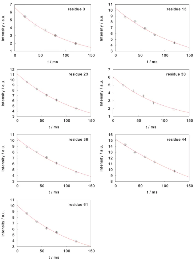
Figure S3. Measured intensity decays in the two-field NMR experiment for the measurement of
carbon-13 longitudinal relaxation rates. Intensities are shown as black crosses together with their experimental uncertainty, the red curves represent the fitted mono-exponential decay.
Figure S4. Measured intensity decays in the two-field NMR experiment for the measurement of
carbon-13 R1ρ relaxation rates. Intensities are shown as black crosses together with their
Figure S5. Measured intensity decays in the two-field NMR experiment for the measurement of
proton longitudinal relaxation. Intensities are shown as black crosses together with their experimental uncertainty, the red curves represent the fitted mono-exponential decay.
Figure S6. Measured intensity decays in the two-field NMR experiment for the measurement of
proton R1ρ relaxation rates. Intensities are shown as black crosses together with their experimental
Correlation function for the analysis of relaxation.
The motions of the CH bond are decomposed into three statistically independent motions. The correlation function 𝐶"#(𝑡) is written as the product of three correlation functions:
𝐶'(𝑡) = 𝐶)*+,'(𝑡)𝐶-.'/(𝑡)𝐶0(𝑡) (S1)
𝐶)*+,'(𝑡) is the correlation function for the fast rotation of the methyl group about its symmetry axis, the subscript i defines the orientation of the principal axis of the interaction under consideration, here 𝑖 ∈ {𝐶𝐻, 𝐶𝐶, 𝐶𝐷, 𝐻𝐷}; 𝐶-.'/(𝑡) describes the motions of the “symmetry” axis of the methyl group aligned with the CC bond; and 𝐶0(𝑡) is the correlation function for overall rotational diffusion of the entire protein or domain. Fast rotation of the methyl group about its symmetry axis is described using the simple model-free correlation function 𝐶)*+,'(𝑡):
𝐶)*+,'(𝑡) = 𝑆)*+,'8 + :1 − 𝑆
)*+,'8 =𝑒𝑥𝑝(−𝑡 𝜏⁄ )*+) (S2)
This rotation is axially symmetric, not isotropic, and the order parameter depends on the angle qi between the principal axis of the interaction and the methyl axis. At equilibrium, all orientations of the methyl group are equally probable, which leads to an order parameter 𝑆)*+,'8 = [(3 cos8𝜃
' − 1) 2⁄ ]8. For the CH dipole-dipole coupling, with an ideal tetrahedral geometry, qCH
= 109.47º, and hence 𝑆)*+,KL8 = 1 9⁄ . We consider that the carbon-13 chemical shift anisotropy tensor is axially symmetric, with a principal axis aligned with the CC bond, and 𝑆)*+,KK8 = 1. Motions of the CC axis are described by the “extended model free” approach, 44-46 with a
correlation function 𝐶-.'/(𝑡): 𝐶-.'/(𝑡) = 𝑆N8𝑆
/8+ :1 − 𝑆N8=exp:−𝑡 𝜏⁄ = + 𝑆N N8 (1 − 𝑆/8)exp(−𝑡 𝜏⁄ ) / (S3)
Motions in two different ranges of correlation times are accounted for in 𝐶-.'/(𝑡): faster (resp. slower) motions are described by the order parameter 𝑆N8 (resp. 𝑆
/8) and the correlation time 𝜏N (resp. 𝜏/). The overall rotational diffusion of the protein is described by an isotropic diffusion tensor defined by a single correlation time tc with a correlation function 𝐶ST(𝑡) =
Figure S7. Parameters for internal dynamics obtained by the analysis of three sets of relaxation
rates. Sf2 and Ss2 are order parameters associated with fast and slow motions of the C 1-C 1 bond,
respectively. Corresponding correlation times are tf and ts. tmet is the correlation time for rotation
of the methyl group. Results of analysis of all methyl group motions published earlier [1] are presented. Analysis of relaxation at 20 magnetic fields [1] all longitudinal relaxation rates measured at fields B0 < 9 T where measured with no rf pulse at low field are shown in rows (a),
(d), (g), (j), (m), (p), and (s) (for detailed description of the dynamics parameters see [1]). Parameters obtained from the analysis of longitudinal, transverse relaxation and dipolar cross-relaxation rates at high field only (9.4 T; 14.1 T; 18.8 T; and 22.3 T) are shown in rows (b), (e), (h), (k), (n), (q), and (t). Analysis of the set of high field relaxation rates complemented by accurate longitudinal and transverse relaxation rates at 0.33 T measured with the two-field spectrometer are shown in rows (c), (f), (i), (l), (o), (r), and (u).
Table S3. Carbon longitudinal and transverse relaxation rates, and carbon-hydrogen dipole-dipole
cross-relaxation rate at 22.3 T (950 MHz proton Larmor frequency) used in the MCMC analysis presented in Fig. S7. The residue number, longitudinal relaxation rate, transverse relaxation rate and carbon-proton cross-relaxation rates are shown in the first, second, and third respectively and were published earlier [1]. Chemical exchange affects relaxation rates of Ile-44 and its transverse relaxation rates were not included in the analysis.
Residue R1 (13C) / s-1 R2 (13C) / s-1 sNOE (13C-1H) /s-1 3 0.25 ± 0.003 2.18 ± 0.02 0.079 ± 0.001 13 0.36 ± 0.004 1.76 ± 0.02 0.113 ± 0.001 23 0.54 ± 0.005 1.90 ± 0.02 0.198 ± 0.002 30 0.29 ± 0.003 2.31 ± 0.02 0.085 ± 0.001 36 0.32 ± 0.003 1.84 ± 0.02 0.087 ± 0.001 44 0.31 ± 0.003 - 0.077 ± 0.001 61 0.42 ± 0.004 2.04 ± 0.02 0.144 ± 0.001
Table S4. Carbon longitudinal and transverse relaxation rates, and carbon-hydrogen dipole-dipole
cross-relaxation rate at 18.8 T (800 MHz proton Larmor frequency) used in the MCMC analysis presented in Fig. S7. The residue number, longitudinal relaxation rate, transverse relaxation rate and carbon-proton cross-relaxation rates are shown in the first, second, and third respectively and were published earlier [1]. Chemical exchange affects relaxation rates of Ile-44 and its transverse relaxation rates were not included in the analysis.
Residue R1 (13C) / s-1 R2 (13C) / s-1 sNOE (13C-1H) /s-1 3 0.27 ± 0.004 2.10 ± 0.02 0.081 ± 0.002 13 0.39 ± 0.003 1.71 ± 0.02 0.119 ± 0.002 23 0.56 ± 0.005 1.88 ± 0.01 0.203 ± 0.003 30 0.32 ± 0.004 2.25 ± 0.02 0.088 ± 0.002 36 0.36 ± 0.003 1.73 ± 0.02 0.092 ± 0.002 44 0.34 ± 0.004 - 0.079 ± 0.002 61 0.44 ± 0.004 1.94 ± 0.02 0.151 ± 0.003
Table S5. Carbon longitudinal and transverse relaxation rates, and carbon-hydrogen dipole-dipole
cross-relaxation rate at 14.1 T (600 MHz proton Larmor frequency) used in the MCMC analysis presented in Fig. S7. The residue number, longitudinal relaxation rate, transverse relaxation rate and carbon-proton cross-relaxation rates are shown in the first, second, and third respectively and were published earlier [1]. Chemical exchange affects relaxation rates of Ile-44 and its transverse relaxation rates were not included in the analysis.
Residue R1 (13C) / s-1 R2 (13C) / s-1 sNOE (13C-1H) /s-1 3 0.34 ± 0.006 2.04 ± 0.02 0.079 ± 0.002 13 0.46 ± 0.005 1.66 ± 0.01 0.121 ± 0.003 23 0.64 ± 0.006 1.84 ± 0.01 0.220 ± 0.004 30 0.40 ± 0.006 2.17 ± 0.02 0.086 ± 0.002 36 0.44 ± 0.005 1.67 ± 0.013 0.096 ± 0.002 44 0.41 ± 0.006 - 0.088 ± 0.002 61 0.51 ± 0.005 1.89 ± 0.01 0.156 ± 0.003
Table S6. Carbon longitudinal and transverse relaxation rates, and carbon-hydrogen dipole-dipole
cross-relaxation rate at 9.4 T (400 MHz proton Larmor frequency) used in the MCMC analysis presented in Fig. S7. The residue number, longitudinal relaxation rate, transverse relaxation rate and carbon-proton cross-relaxation rates are shown in the first, second, and third respectively and were published earlier [1]. Chemical exchange affects relaxation rates of Ile-44 and its transverse relaxation rates were not included in the analysis.
Residue R1 (13C) / s-1 R2 (13C) / s-1 sNOE (13C-1H) /s-1 3 0.49 ± 0.04 2.22 ± 0.10 0.077 ± 0.009 13 0.62 ± 0.03 1.67 ± 0.08 0.125 ± 0.011 23 0.74 ± 0.03 1.90 ± 0.07 0.229 ± 0.017 30 0.57 ± 0.04 2.29 ± 0.10 0.091 ± 0.010 36 0.62 ± 0.03 1.75 ± 0.08 0.108 ± 0.010 44 0.52 ± 0.03 - 0.110 ± 0.010 61 0.62 ± 0.03 2.05 ± 0.07 0.162 ± 0.013
Table S7. Median values and standard deviations for fitted parameters shown in the distributions in Figure S7 “all fields”. Results were obtained after a Markov-Chain Monte-Carlo on corrected high-resolution relaxometry data and high-field data.
SX8 S
Y8 CSA (ppm)
Median +s -s Median +s -s Median +s -s
3 0.71 0.01 0.01 0.76 0.12 0.15 23.8 1.57 1.43 13 0.63 0.02 0.03 0.62 0.06 0.15 23.9 2.53 2.33 23 0.51 0.01 0.01 0.90 0.07 0.12 20.1 1.36 1.37 30 0.81 0.01 0.02 0.74 0.10 0.30 22.5 2.05 2.19 36 0.67 0.02 0.02 0.58 0.03 0.03 29.4 1.28 1.19 44 0.51 0.03 0.05 0.28 0.02 0.03 Not fitted 61 0.55 0.02 0.01 0.89 0.07 0.11 26.1 1.87 1.83 tmet (ps) tf (ps) ts (ns)
Median +s -s Median +s -s Median +s -s
3 8.56 1.06 0.88 34.8 24.4 17.0 17.7 8.86 10.6 13 11.5 1.85 0.94 77.3 40.7 39.3 3.13 4.10 1.08 23 21.7 0.38 0.33 150 11.8 12.1 18.3 8.37 11.4 30 9.03 0.92 0.61 61.8 47.6 35.4 6.98 14.8 4.20 36 8.05 1.14 0.43 82.8 24.8 37.6 2.48 0.63 0.45 44 5.58 2.44 1.17 70.3 42.1 42.9 1.27 0.36 0.22 61 14.4 0.71 0.45 138 18.2 26.1 17.3 9.05 12.7
Table S8. Median values and standard deviations for fitted parameters shown in the distributions in Figure S7. Results were obtained after a Markov-Chain Monte-Carlo high-field data only. CSA was kept constant to the median value shown in Table S7.
𝑆N8 𝑆 /8 Median +s -s Median +s -s 3 0.70 0.01 0.01 0.78 0.12 0.14 13 0.64 0.03 0.03 0.34 0.27 0.24 23 0.54 0.03 0.03 0.71 0.20 0.33 30 0.83 0.02 0.04 0.40 0.28 0.25 36 0.71 0.03 0.03 0.37 0.23 0.25 44 0.70 0.20 0.20 0.63 0.28 0.35 61 0.60 0.03 0.04 0.54 0.25 0.29 tmet (ps) tf (ps) ts (ns)
Median +s -s Median +s -s Median +s -s
3 8.76 1.00 0.89 30.8 19.8 14.2 20.8 6.61 9.56 13 11.4 1.07 0.52 91.2 27.4 33.6 8.98 4.70 4.97 23 22.2 0.82 0.49 136 18.5 23.0 19.2 7.62 10.6 30 9.26 0.66 0.48 65.3 2x10³ 36.1 18.1 7.53 8.42 36 8.21 0.66 0.38 114 34.8 41.4 6.50 4.28 3.76 44 8.56 1.04 2.37 3x10³ 16x103 3x10³ 21.2 6.38 15.8 61 15.2 1.08 0.57 103 30.2 25.6 19.9 6.69 9.66
Table S9. Median values and standard deviations for fitted parameters shown in the distributions in Figure S7. Results were obtained after a Markov-Chain Monte-Carlo on accurate carbon longitudinal and transverse relaxation rates at 0.33 T measured in this study and high-field data.
𝑆N8 𝑆 /8 Median +s -s Median +s -s 3 0.69 0.02 0.23 0.71 0.16 0.42 13 0.64 0.02 0.03 0.43 0.22 0.29 23 0.54 0.03 0.03 0.70 0.20 0.29 30 0.83 0.02 0.02 0.36 0.32 0.24 36 0.69 0.03 0.06 0.55 0.10 0.30 44 0.51 0.02 0.03 0.28 0.07 0.11 61 0.61 0.03 0.04 0.40 0.28 0.26 tmet (ps) tf (ps) ts (ns)
Median +s -s Median +s -s Median +s -s
3 8.31 1.08 0.90 45.0 9x10³ 23.9 21.5 6.33 8.81 13 11.3 0.92 0.52 91.6 28.7 31.6 6.74 5.96 3.76 23 22.2 0.71 0.48 132 16.6 22.6 19.9 7.16 10.1 30 9.34 0.72 0.49 53.3 35.6 29.4 19.0 7.03 10.0 36 8.29 1.29 0.56 105 82.8 53.9 3.38 5.43 1.68 44 5.85 1.43 0.74 74.1 35.1 28.3 1.83 1.43 0.50 61 15.4 1.26 0.68 94.4 33.6 30.0 20.0 6.73 9.33 Reference:
[1] Cousin, S.F.; Kadeřávek, P.; Bolik-Coulon, N.; Gu, Y.; Charlier, C.; Carlier, L.; Brüschweiler-Li, L.; Marquardsen, T.; Tyburn, J.M.; Brüschweiler, R.; Ferrage, F., Time-resolved protein side-chain motions unraveled by high-resolution relaxometry and molecular dynamics simulations J. Am. Chem. Soc. 2018, 140, 13456-13.


![Table S2. Proton longitudinal and transverse relaxation rates. The residue number, longitudinal relaxation rate, transverse relaxation rate, predicted longitudinal and transverse relaxation rates simulated using dynamic parameters published earlier [1] a](https://thumb-eu.123doks.com/thumbv2/123doknet/11365344.285677/16.918.108.782.587.844/longitudinal-transverse-relaxation-longitudinal-relaxation-transverse-relaxation-longitudinal.webp)