THÈSE DE DOCTORAT
Présentée pour obtenir le grade de Docteur en Sciences de l’Université Mohammed V-Agdal Faculté des sciences-Rabat
Abdelhak MAHMOUDI Discipline: Science de l’ingénieur
Spécialité: Informatique
Machine Learning Using Support Vector Machines: Application
to Human Brain Decoding and Weld Flaws Classification
Soutenue le 07 Octobre 2013 Devant le jury:
Président:
M. El-Houssine BOUYAKHF, PES, Faculté des Sciences, Rabat, Maroc Examinateurs:
Mme. Fakhita REGRAGUI, PES, Faculté des Sciences, Rabat, Maroc M. Samir BENNANI, PES, EMI, Rabat, Maroc
M. Abdelaziz BOUROUMI, PES, Faculté des Sciences, Ben M’sik, Maroc M. Mohammed Majid HIMMI, PES, Faculté des Sciences, Rabat, Maroc Invités:
M. Andrea BROVELLI, Dr. Chercheur INT-CNRS, Marseille, France M. Rachad ALAMI, Dr. Chef DIAI, CNESTEN, Rabat, Maroc
Faculté des Sciences, 4 Avenue Ibn Battouta B.P. 1014 RP, Rabat – Maroc Tel +212 (0) 37 77 18 34/35/38, Fax : +212 (0) 37 77 42 61, http://www.fsr.ac.ma
FACULTÉ DES SCIENCES
Rabat
Les travaux présentés dans ce mémoire ont été effectués au sein du laboratoire d’Informatique, Mathématiques appliquées, Intelligence Artifi-cielle et Reconnaissance des Formes (LIMIARF) à la Faculté des Sciences de l’université Mohammed V-Agdal, Rabat, Maroc. Un premier stage de recherche a été effectué en collaboration avec la division Instrumentation et Applications Industrielles (DIAI) du Centre National de l’Energie, des Sciences et des Techniques Nucléaires (CNESTEN). Un deuxième stage de recherche a été réalisé dans le cadre du projet Européen Neuromed en col-laboration avec l’Institut des Neurosciences Cognitives de la Méditerranée (INCM) (actuellement l’Institut des Neurosciences de la Timone (INT) d’Aix Marseille université).
Qu’il me soit permis d’adresser ma vive gratitude et ma profonde recon-naissance au Directeur de cette thèse, Madame Fakhita REGRAGUI, pro-fesseur de l’enseignement supérieur à la Faculté des Sciences de Rabat, pour la confiance qu’elle m’a témoignée le long de ce travail. Sa disponibilité et son constant souci de faire avancer nos recherches m’ont poussé à donner le meilleur de moi-même. Sa lecture attentive de ce document, ses conseils et ses remarques judicieux ont grandement aidé à améliorer ce mémoire. Je la remercie aussi de sa présence parmi le jury de cette thèse.
Je suis particulièrement reconnaissant à Monsieur El Houssine BOUYAKHF, professeur de l’enseignement supérieur à la Faculté des Sciences de Rabat et Directeur du laboratoire LIMIARF pour m’avoir accueilli au sein de son laboratoire, pour sa gentillesse et pour sa confiance dont j’espère avoir été à la hauteur. Je le remercie aussi de m’avoir fait l’honneur de présider le jury de cette thèse.
Mes remerciements vont également à Monsieur Mohammed Majid HIMMI, professeur de l’enseignement supérieur à la Faculté des Sciences de Rabat. Merci pour vos encouragements de tous les jours et d’avoir accépté de juger ce travail.
Mes reconnaissances vont également à Monsieur Samir BENNANI, pro-fesseur de l’enseignement supérieur à l’Ecole Mohammedia d’ingénieurs de l’université Mohammed V-Agdal, Rabat, qui a bien accepté d’être rapporteur de cette thèse, pour sa lecture minutieuse et ses remarques. Je le remercie aussi de bien vouloir siéger parmi les membres du jury.
Je tiens aussi à remercier Monsieur Abdelaziz BOUROUMI, professeur de l’enseignement supérieur à la Faculté des Sciences Ben M’sik de l’université Hassan II Mohammedia-Casablanca d’avoir accepté d’être rapporteur de cette thèse. Je ne peux que lui être reconnaissant et je le remercie pour son aide, pour les riches discussions que nous avons eues. Je le remercie de même que
plications Industrielles (DIAI) du Centre National de l’Energie, des Sciences et des Techniques Nucléaires (CNESTEN). Je tiens à exprimer ma profonde gratitude pour l’honneur qu’il me fait en acceptant de juger mon travail et d’avoir accepté mon invitation à siéger parmi les membres de jury de cette thèse.
A Monsieur Andrea BROVELLI, chercheur à l’Institut des Neurosciences de la Timone (INT) d’Aix Marseille université. Je tiens à le remercier pour son encadrement pendant mes huit mois de stages à l’Institut des Neurosciences Cognitives de la Méditerranée (INCM) dans le cadre du projet Neuromed. C’est un honneur qu’il me fait en acceptant d’évaluer ce travail et d’avoir accepté d’être membre de jury de cette thèse.
Ma gratitude à Monsieur Driss BOUSSAOUD, Ex-Directeur de l’Institut des Neurosciences Cognitives de la Méditerranée (INCM) pour m’avoir ac-cueilli dans son établissement et de m’avoir permis de travailler dans une équipe de chercheurs internationaux. Merci de m’avoir soutenu chaque fois qu’il était nécessaire.
A Monsieur Khalid El MEDIOURI, Directeur Général du Centre Na-tional de l’Energie, des Sciences et des Techniques Nucléaires (CNESTEN), de m’avoir accueilli pendant quelques mois au CNESTEN.
Pour votre patience, votre confiance, votre dévouement,
votre amour,
Je vous aime.
A mes soeurs, Najat et Safae et mon frère Omar,
A mon frère Amine et ma belle-soeur Asmae
Avec mes toutes petites adorables nièces, Tasnime et Nour,
Pour votre soutien et tout le bonheur que vous m’apportez.
Je vous aime aussi.
A toute ma famille
Mes tantes et oncles, mes cousines et cousins,
A tous mes amis
1 Introduction 1
2 Machine Learning 5
2.1 Introduction . . . 5
2.2 Learning a function . . . 6
2.2.1 Regression versus classification. . . 7
2.2.2 Linear separability . . . 9
2.2.3 Unsupervised versus supervised learning . . . 9
2.3 Supervised classifiers . . . 11
2.3.1 Instance based classifiers . . . 11
2.3.2 Logic based classifiers: Decision trees . . . 13
2.3.3 Perceptron based classifiers . . . 16
2.3.4 Statistical based classifiers . . . 19
2.3.5 Support Vector Machines. . . 21
2.4 Data processing . . . 21
2.4.1 Data-set balance . . . 22
2.4.2 Dimensionality reduction . . . 25
2.5 Model selection . . . 30
2.5.1 Example of bias-variance tradeoff . . . 30
2.5.2 Cross Validation . . . 31
2.6 Classifier performance evaluation . . . 33
2.6.1 Accuracy metric . . . 33
2.6.2 Receiver Operating Characteristic (ROC) Curve . . . . 34
2.7 Conclusion . . . 35
3 Mathematical basis of the support vector machines 37 3.1 Introduction . . . 37
3.2 Mathematical basis of Support Vector Machines . . . 38
3.2.1 Linear SVM . . . 38
3.2.2 Non Linear SVM . . . 41
3.3 Why does SVM works well? . . . 43
3.4 Finding SVM optimal parameters . . . 45
3.5 Feature selection using linear SVM-RFE . . . 46
4 Decoding functional magnetic resonance images of brain 47
4.1 Introduction . . . 47
4.2 The fMRI experiment. . . 48
4.3 From univariate to multivariate analysis . . . 50
4.3.1 Univariate analysis of fMRI data: The GLM approach 50 4.3.2 Multivariate analysis of fMRI data: The MVPA approach 54 4.4 MVPA as a classification problem . . . 54
4.4.1 Which classifier to use? . . . 54
4.4.2 Dimensionality reduction . . . 55
4.4.3 N-fold cross-validation . . . 57
4.4.4 Performance estimation of SVM using ROC . . . 58
4.4.5 Nonparametric permutation test analysis . . . 58
4.5 Decoding fMRI data using searchlight analysis . . . 59
4.5.1 Experimental design . . . 60
4.5.2 The proposed multivariate searchlight implementation. 61 4.6 Conclusion . . . 67
5 Weld flaws classification 69 5.1 Introduction . . . 69
5.2 Detection of flaw candidates . . . 72
5.2.1 Weld bead isolation . . . 72
5.2.2 Flaws detection using local thresholding . . . 76
5.2.3 Other results . . . 79
5.3 Flaws classification . . . 79
5.3.1 Weld flaws features extraction . . . 81
5.3.2 SMOTE to correct data-set unbalance . . . 85
5.3.3 Feature selection using CV-SVM-RFE . . . 85
5.3.4 Classification using linear SVM . . . 86
5.3.5 Results and discussion . . . 86
5.4 Conclusion . . . 94
6 Conclusion 95 6.1 Summary of contributions . . . 95
6.2 Research perspectives . . . 96
A List of publications 99 A.1 International journals . . . 99
A.2 International conferences . . . 99
2.1 Linear regression. . . 8
2.2 Linear classification. . . 8
2.3 Linearity versus non linearity. . . 10
2.4 Supervised versus unsupervised learning. . . 10
2.5 Nearest mean classifier. . . 12
2.6 K-nearest neighbor classifier. . . 12
2.7 Decision tree. . . 16
2.8 Single layered perceptron. . . 17
2.9 Artificial neural network. . . 18
2.10 Data-set unbalance . . . 23
2.11 Curse of dimensionality . . . 26
2.12 Principal component analysis. . . 29
2.13 Bias-variance tradeoff. . . 32
2.14 Confusion matrix. . . 34
2.15 ROC curve representation. . . 35
3.1 Support vector machine illustration. . . 38
3.2 Effect of C on the decision boundary. . . 40
3.3 Decision boundary with polynomial kernel. . . 43
3.4 Decision boundary with RBF kernel. . . 44
3.5 Grid and pattern search. . . 45
4.1 Typical fMRI experiment. . . 49
4.2 Event-related versus blocked deign. . . 50
4.3 Stimuli function convolution with the HRF. . . 52
4.4 Thresholded statistical map. . . 53
4.5 Cross-validation schemes . . . 57
4.6 Experimental design of arbitrary visuomotor learning. . . 60
4.7 Label vector design. . . 62
4.8 AUC performance map of the searchlight analysis. . . 63
4.9 2D Illustration of the "searchlight" method. . . 64
4.10 ROC analysis of simulated data. . . 65
4.11 Non-parametric analysis results. . . 66
5.1 X-ray radiography. . . 69
5.2 Weld bead extraction steps. . . 73
5.3 An original X-ray image. . . 73
5.5 Otsu’s thresholding.. . . 76
5.6 Weld bead isolation. . . 76
5.7 Homogenous image. . . 78
5.8 Sauvola’s thresholding. . . 79
5.9 Influence of the window’s size. . . 80
5.10 Results flaw/Non-Flaw. . . 80
5.11 Results Circular flaw. . . 81
5.12 Results linear flaw. . . 81
5.13 Classification analysis steps. . . 83
5.14 Analyzes results. . . 92
1 FKNN algorithm . . . 14
2 SVM-RFE algorithm . . . 46
3 SVM-ROC algorithm . . . 58
Introduction
Nowadays, machine learning (ML) is a powerful technology that can be ap-plied to several real-world problems including object, speech and handwriting recognition, medical diagnosis, spam classification, robotics, sentiment anal-ysis, computational finance, etc. It involves the question "how can one build computer programs that automatically improve their performance through experiences?". Concretely, in a variety of real-world problems, the core of ML deals with modeling and generalization. Modeling consists of inferring a function (a model) that describes a subset of collected data examples from experiences. Generalization is the property that the model will perform well on unseen subset of data examples.
Learning from data is a big challenge despite of its apparent simplicity. In fact, the generalization performance of a learning algorithm depends on many parameters: the nature of the learning task, the data dimensionality and distribution, the chosen learning model, the performance measurement metric, etc. Therefore, crucial choices have to be carried out to achieve the desired performance.
Depending on the fact that the collected data could be associated with a label or not, learning can be supervised or unsupervised. Supervised learning infers a function from labeled data while unsupervised learning consists in finding hidden structures in unlabeled data. Other types of learning exist such as semi-supervised and reinforcement learning [Kaelbling 1996].
In this work we were mostly interested in supervised classification where data are associated with discrete labels. One of the most powerful supervised classifiers is the support vector machine (SVM) classifier which proved to per-form an excellent generalization perper-formance in many applications compared to other classifiers [Vapnik 1995]. The generalization properties of SVM do not depend on the dimensionality of the data space, in both cases of balanced or unbalanced data. In addition, SVM can be wrapped efficiently into a fea-ture selection algorithm to perform feafea-ture rankings. Therefore, SVM is now one of the standard tools available for ML.
In light of the above, we attempted to use the SVM properties in two applications: (1) Human brain decoding using functional magnetic resonance imaging (fMRI) for neuroscience tasks; (2) Weld flaws detection and classification using X-Ray images for non-destructive testing (NDT) tasks.
Human brain decoding
Decoding human brain fascinates more and more the community of neuroscientists [Haynes 2006, van Gerven 2013]. The brain can be viewed as a system (a model) that maps stimuli (inputs) into brain activity (outputs). Under this assumption, human brain decoding consists of using brain activity to predict information about the stimuli. One of the most used techniques to measure brain activity is fMRI. This technique exploits blood-oxygen-level-dependent (BOLD) contrasts to map neural activity associated with the brain functions in each voxel in the brain. The BOLD signal may be analyzed either at each voxel independently (univariate analysis) or at spatial pattern of voxels (multivariate analysis). One of the limitations of univariate analysis is the assumption that the covariance across neighboring voxels is not informative about the cognitive function under examination
[Friston 1995, Kriegeskorte 2006]. Multivariate methods represent more
promising techniques that are currently exploited to investigate the informa-tion contained in distributed patterns of neural activity to infer the funcinforma-tional role of brain areas and networks. They are based on ML algorithms and are known as multi-voxel pattern analysis (MVPA). MVPA is considered as a supervised classification problem where the classifier attempts to capture the relationships between spatial pattern of fMRI activity and stimuli. In a review paper related to MVPA, we showed that the most important challenges concern the high-dimensional input structure of the acquired fMRI data and the interpretability of the obtained results [Mahmoudi 2012]. The choice of the SVM classifiers is appropriate in this case since they generalize well even in high-dimensional feature space. In addition, when used in their linear form, SVMs produce linear boundaries in the original feature space, which makes the interpretation of the results straightforward.
Weld flaws detection and classification
Non destructive testing (NDT) is a set of techniques used in industry to evaluate the properties of a material or a component without causing damage. In the current industrial practice, radiography testing (RT) remains among the most adapted NDT processes widely used for detecting and classifying flaws resulting from welding operations, very often detrimental to the integrity of welded components. RT can be carried out using X-or γ-rays producing radiographs of the exposed welded component with reflected flaws which may exhibit features linked to morphology, position, orientation, size, etc. Experts in NDT have the ability to visually interpret
radiographs by assigning the detected flaws to different classes including cracks (C), linear inclusions (LI), lack of penetration (LP) and porosities (PO), etc. However, such conventional interpretation of radiographs is a very expensive process while being slow and subject to errors. In 1975, a weld radiograph was digitized for the first time and with the advance in digital image processing techniques, the first automatic inspection system (AIS) was developed [Snyder 1975]. In the last few years, ML algorithms were introduced to contribute and build more powerful and optimized AISs in terms of performance, time and cost.
Generally, a weld flaws AIS consists of two main stages: flaws detection and flaws classification. Flaws detection stage involves two steps: the image preprocessing step seeking to improve the quality of the image and the seg-mentation step allowing to detect the weld flaws candidates. Researchers used various traditional preprocessing and segmentation approaches which are often complex and require more computing time [Liao 2009,Lim 2007,Wang 2008]. In this work we propose to use global and local thresholding allowing more ef-ficiency in terms of computing complexity [Mahmoudi 2008,Mahmoudi 2009]. Flaws classification involves three steps: feature extraction, fea-ture selection and classification. For feature extraction, several types of features have been used such as geometric-based features
[Wang 2002, Shafeek 2004, Da-Silva 2005, Liao 2003b, Liao 1998],
moment-based features [Nacereddine 2006] and texture-based features
[Kasban 2011, Mery 2003]. In the feature selection step, several
meth-ods were proposed in the literature such as correlation-based methmeth-ods
[Liao 2003a], sequential forward selection (SFS) method [Mery 2003],
prin-cipal components analysis (PCA) [Vilar 2009] and ant colony optimization (ACO)-based methods [Liao 2009]. Instead, the recursive feature elimination (RFE) method can be chosen as an alternative for features selection due to its high performance [Guyon 2002]. Nonetheless, RFE is data-dependant. We propose in this case to combine RFE with SVM and introduce the cross-validation procedure to make feature selection data independent. Finally, in the classification step, most of the researchers used the artificial neural network (ANN)-based algorithms [Khandetsky 2002, Wang 2002,
Nacereddine 2006, Lim 2007, Zapata 2010, Kasban 2011]. Recent research
are interested in the use of SVMs due to their high generalization performance
[Wang 2008, Valavanis 2010, Domingo 2011]. However, only a few authors
addressed the data-set unbalance problem [Hernández 2004,Liao 2008] which limits the application of the SVM classifiers [Akbani 2004]. In this work, we show that an AIS can improve its generalization performance through the SVMs using appropriate features selection whether in balanced or unbalanced set of data environment [Mahmoudi 2013].
Brief overview of the chapters
This dissertation comprises six chapters briefly described as follows:
In chapter2, we first define some terminologies generally used in ML com-munity. Second, we give a brief survey of some powerful supervised classifiers. Third, we discuss two main data preprocessing techniques: data unbalance correction and dimensionality reduction. Fourth, we focus on the problem of model selection and conditions under which learning data can be guaran-teed. Finally, we present and discuss metrics used to estimate the classifier generalization performance.
Chapter 3 is devoted to SVM classifiers. After a brief introduction of linear and non-linear SVMs from a theoretical perspective, we attempt to answer the question of why SVMs work well. We then describe some methods used to find SVMs optimal parameters. Finally, we introduce the SVM-based recursive feature elimination algorithm (SVM-RFE) to find relevant features allowing better generalization performance.
Chapter 4 deals with the application of the above mentioned techniques to decode fMRI signals acquired during a functional neuroimaging task. We first describe a typical fMRI experiment. Second, we report the limitations of univariate analysis and present MVPA as a solution to decode functional neuroimaging data. Third, we discuss the recommendations necessary to per-form MVPA analysis. These includes the choice of the classifier, dimensional-ity reduction, cross-validation scheme, performance estimation and the non-parametric permutation test analysis. Based on the above, we implement a method called searchlight to decode fMRI data of an arbitrary visuomotor learning task and give illustration of the obtained results.
In chapter 5, we apply machine learning using SVM to the detection and classification of weld flaws. We first describe the proposed method that allows the detection of weld flaws using image processing techniques. Second, we suggest a set of analyzes that allow an automatic inspection system to improve its generalization performance. These analyzes include balancing the data using Synthetic Minority Over-sampling Technique (SMOTE) and selecting the features using cross-validated SVM-RFE.
Machine Learning
2.1
Introduction
Learning is difficult to be defined precisely. According to the psychologist Peter Gray [Gray 2010], learning is defined broadly as "any process through which experience at one time can alter an individual’s behavior at a future time.". Some dictionaries state that: "Learning is the most general term referring to knowledge obtained by systematic study or by trial and error". Others tell us that: "Learning is the activity or process of gaining knowledge or skill by studying, practicing, being taught, or experiencing something".
Very often, concepts being explored by psychologists illuminate certain aspects for mathematicians and physicists and vise versa. In 1959, Arthur Samuel defined a new field called machine learning as "the field of study that gives computers the ability to learn without being explicitly programmed". In 1997, Tom Mitchell gives an explicit definition stating that "A computer program is set to learn from an experience E with respect to some task T and some performance measure P if its performance on T as measured by P improves with experience E".
Concretely, in a variety of real-world problems, big amount of data are collected and need to be learned. Machines (computer programs) seem to be powerful tools to perform such a learning. In other words, given data ex-amples, the core of ML deals with modeling and generalization. Modeling consists of inferring a function (a model) that describes a subset of data ex-amples. Generalization is the property that the model will perform well on unseen subset of data examples.
Depending on the fact that data examples are labeled or unlabeled, learn-ing from data can be supervised or unsupervised. Supervised learnlearn-ing infers a function from labeled data while unsupervised learning refers to the problem of trying to find hidden structures in unlabeled data. Other types of learn-ing includes semi-supervised learnlearn-ing which combines both labeled and unla-beled examples to generate an appropriate function and reinforcement learn-ing where the algorithm learns a policy of how to act given an observation of the world. Every action has some impact in the environment, and the environ-ment provides feedback that guides the learning algorithm [Kaelbling 1996].
It is also useful to distinguish between two main supervised models: clas-sification models (classifiers) and regression models. Classifiers map the input space into pre-defined class labels. On the other hand, regression models map the input space (data examples) into a real-value domain ref.
Learning from data is a big challenge despite of its apparent simplicity. In fact, the generalization performance of a learning algorithm depends on many parameters: the nature of the learning task, the data’s dimensionality and distribution, the chosen learning model, the performance measurement metric, etc. Therefore, crucial choices have to be carried out.
This chapter focuses on supervised learning as a classification problem. In section 2.2, we first begin by defining some terminologies generally used in ML. In section2.3, we give a brief survey of some known supervised classifiers. Section 2.4 discusses data preprocessing techniques including data unbalance correction and dimensionality reduction. Section2.5focuses on the problem of model selection and conditions under which learning data can be guaranteed. Finally, in section 2.6, two metrics to estimate the classifier generalization performance are presented and discussed.
2.2
Learning a function
Imagine that there is a function f of a vector-valued input x of n elements x = (x1, ..., xn). The task of the learner is to guess what is the output f (x).
Let h be the hypothesis about the function to be learned. h is selected from a class of functions H by training the learner using a sub-set of examples called "training-set". Another set called "test-set" is used in order to test the performance of h in predicting the correct output.
It is worth mentioning that ML community uses different terminologies. For example, the input vector is called by a variety of names. Some of these are: input vector, pattern vector, feature vector, sample, example, and in-stance. The components, xi, of the input vector are variously called features,
attributes, input variables, and components. The output vector may be called the target variable, label or class.
For more coherence in this thesis report, we will assume the following notations and terminologies:
• Example: the input vector. • m: the number of examples.
• x(i): the i-th example (i∈ {1, ..., m})
• n: the number of features.
• xj: the j-th feature of the example x (j ∈ {1, ..., n}).
• x(i)j : the j-th feature of the i-th example.
• y(i): the output of the i-th example.
2.2.1
Regression versus classification
The output vector y may be a real number (y ∈ IR) or a discrete value (for instance y ∈ {1, −1}). In the first case, the learning problem is called "regres-sion". The process embodying the function h is called a function estimator, and the output is called an output value or estimate.
Regression is the problem of predicting a real-valued function from training examples Fig.2.1. In its linear form, suppose the input features of an example x(i) are x(i)
1 , ..., x (i)
n . A linear function of these features is of the form:
f (x(i)1 , ..., x(i)n ) = w0+ w1x1(i)+ ...wjx(i)j + ... + wnx(i)n (2.1)
where w = {w0, w1, ..., wn} is a tuple of weights providing that x(i)0 = 1.
The objective of linear regression is to find the weight vector w that min-imizes the following sum-of-squares error:
J(w) =
m
∑
i=1
(f (x(i))− y(i))2 (2.2) The weights that minimize J can be computed analytically. A more general approach, which can be used for wider classes of functions, is to compute the weights iteratively. Several methods are used for this end, the simplest one is the Gradient Descent algorithm [Zinkevich 2010].
Alternatively, when the output y is a discrete value (for instance y ∈ {1, −1}), the learning problem is called "classification", the process embody-ing h is variously called a "classifier " and the output itself is called a label, a class, or a decision.
Classification consists in determining the decision function f that takes the values of various features in the data example x and predicts the class of that example (Fig. 2.2). Training will then consists of modeling the relationship between the features and the class label by assigning a weight w to each feature. This weight corresponds to the relative contribution of the feature to successfully classifying two or more classes. When more than two classes are present, the problem can be transformed into a combination of multiple two-class problems (i.e., each class versus all the others).
Figure 2.1: Linear regression.
2.2.2
Linear separability
In geometry, two sets of points in a 2-dimensional space are linearly separable if they can be completely separated by a single line. In general, two sets of examples are linearly separable in n-dimensional space if they can be separated by a hyperplane.
In the field of machine learning, classifiers that perform decision based on the value of a linear combination of the features are called linear classifiers.
In more mathematical terms: Let X1and X2 be two sets of examples in an
n-dimensional feature space. Then X1 and X2 are linearly separable if there
exists n + 1 real numbers w1, w2, .., wn, b, such that every point x(i) ∈ X1,
i∈ {1, ..., m} satisfies:
n
∑
j=1
wjx(i)j ≥ b (2.3)
and every point x(i) ∈ X2 satisfies: n
∑
j=1
wjx(i)j ≤ b (2.4)
where x(i)j is the j-th component of x(i) (j ∈ {1, ..., n}).
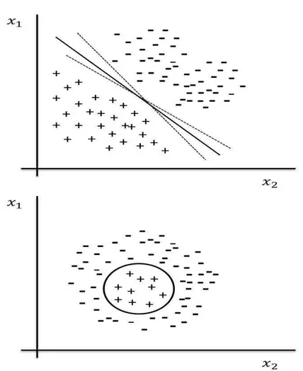
Linear classifiers at first seems trivial, however, the difficulty is in deter-mining the parameters w and b based on the training-set. Indeed, there is an infinite number of linear separators as illustrated by Fig. 2.3. In such case, we need a criterion for selecting among all decision hyperplanes that perfectly separate the training data.
Alternatively, classifiers that perform decision based on a non-linear com-bination of the features are called linearly inseparable classifiers. Those are used when no good linear separator between the classes exists (Fig. 2.3).
2.2.3
Unsupervised versus supervised learning
Since learning involves an interaction between the learner and the environ-ment, one can divide learning tasks according to the nature of that interaction. There are two major settings in which we wish to learn a function (Fig.2.4). In the first learning called unsupervised learning, we simply have a training-set without function values for them. The problem in this case, typically, is to partition the training-set into clusters, C1, ..., Ck, in some appropriate
way. Hence, the objective is to find patterns in the available input data. For example, consider the task of email anomaly detection, all the learner gets as training-set is a large body of email messages and the learner’s task is
Figure 2.3: Linearity versus non linearity. Data in top are linearly separable while data in bottom are linearly inseparable.
Figure 2.4: Supervised versus unsupervised learning. Left data are unlabeled (unsupervised learning). Right, data are labeled (supervised learning).
to detect "unusual" messages. Algorithms commonly used for unsupervised learning include: k-means, self-organizing map (SOM), adaptive resonance theory (ART), etc [Kohonen 1982,Carpenter 1987].
In the second learning called supervised learning, we know the values of f for the examples in the training-set. We assume that if we can find a hypothesis h, that closely agrees with f for the elements of this training-set, then this hypothesis will be a good guess for f . The objective is to learn how to generalize from what has been taught, i.e., to give the correct answer to previously unknown questions. As an illustrative example, consider the task of learning to detect spam email. If the learner receives training emails for which the label spam/not-spam is provided it should figure out a rule for labeling a newly arriving email message.
In this thesis, we will focus on supervised learning. Hereafter we will give brief survey of the commonly used supervised classifiers.
2.3
Supervised classifiers
2.3.1
Instance based classifiers
2.3.1.1 Nearest mean classifier
The nearest mean classifier finds the centroid of a given class and stores it for later classification of test examples. Given a set of m training examples in a c-class problem (c the number of classes) with each class Cl (l = 1...c), having
ml elements, the centroid of class l can be computed as follows:
ol = 1 ml ∑ x(i)inC l x(i) (2.5)
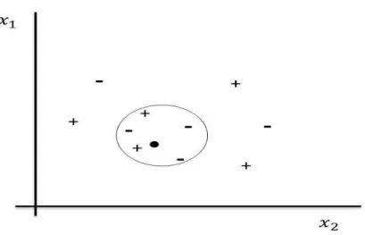
In the classification phase, an unseen test example x is assigned a class label among the classes associated to the stored centroids for which the Euclidean distance from x is the smallest (Fig. 2.5).
2.3.1.2 K-nearest neighbor classifier (KNN)
The k-nearest neighbor classifier assigns an unseen test example to the class represented by the majority of its k-nearest neighbors [Cover 1967]. k is a user-defined constant and the term "nearest" is quantified by a metric measure, usually the Euclidean distance (Fig. 2.6).
To demonstrate a KNN analysis, let’s consider the task of classifying a test example among a number of known examples. This is shown in Fig. 2.6, which depicts the examples with the (+) and (-) symbols and the test example
Figure 2.5: Nearest mean classifier. Data in red color are centroids of each cluster. The unseen example (filled circle) is classified as positive because it is closed to the positive centroid.
Figure 2.6: K-nearest neighbor classifier. The circle groups the k-nearest (k = 5) neighbors of the unseen test example (filled circle). Since the number of negative examples (3) is greater than the number of positive examples (2) within the circle, the unseen example is assigned to the negative class.
with a dark circle. The task is to classify the outcome of the test example based on a selected number of its nearest neighbors. In other words, we want to know whether the test example can be classified as a (+) or (-).
To proceed, let’s consider the outcome of KNN based on 1-nearest neigh-bor. It is clear that in this case 1NN will predict the outcome of the test example with a (+) (since the closest point carries a (+)). By increasing the number of nearest neighbors to 2, the 2NN will not be able to classify the outcome of the test example since the second closest point is a (-), and so both the (+) and the (-) examples achieve the same score (i.e., win the same number of votes). Finally, increasing the number of nearest neighbors to 5 (5NN); will define a nearest neighbor region, which is indicated by the circle. Since there are 2 (+) and 3 (-) examples in this circle, 5NN will assign a (-) to the outcome of the test example.
2.3.1.3 Fuzzy KNN classifier
The fuzzy KNN classifier assigns membership values µl to an unseen test
example x indicating its belongingness to all classes rather than assigning it to a particular class only as in KNN [Keller 1985]. Given a set of m training examples x(i)(i ={1...m}) in a c-class problem, the membership value in the
class l (l ={1...c}) of x are expressed as follows:
µl(x) = ∑k i=1µli(1/||x − x(i)|| 2 (m−1)) ∑k i=1(1/||x − x(i)|| 2 (m−1)) (2.6) where µli denotes the membership of the i-th nearest neighbors in the l-th
class, which is usually known or can be determined beforehand. The following is the fuzzy KNN algorithm:
2.3.2
Logic based classifiers: Decision trees
Decision trees are trees that classify examples by sorting them based on the feature values. Each node in a decision tree represents a feature in an example to be classified, and each branch represents a value that is assigned to the node. Examples are classified starting at the root node and sorted based on their feature values.
The classification begins from the root node. The best feature is used to divide the training-set and the procedure is then repeated on each partition of the divided data, creating sub-trees until the training-set is divided into subsets of the same class. The term best is defined as how well the feature splits the actual set into homogeneous subsets that have the same label. In other terms, the best feature splits the examples into subsets that are (ideally)
Algorithm 1 FKNN algorithm
Input a test example x of unknown classification. Set k, 1 < k < m
Initialize i = 1
while Not all the k-nearest neighbors of x found do Compute distance from x to x(i)
if i < k then
Include x(i) to the set of k-nearest neighbors.
else(x(i) closest to x than any previous nearest neighbor)
Delete the farthest of the k-nearest neighbors. Include x(i) to the set of k-nearest neighbors.
end if end while Initialize l = 1 while l <= c do
Compute the membership value µl using Eq. 2.6.
Increment l; end while
Assign x to the class with the highest µl.
"all positive" or "all negative". Information gain is a common metric used by different decision tree algorithms to find the such features.
Let consider the two class classification problem and suppose the training-set contains m examples ( m+ positive and m−negative) (i.e., m = m++m−).
The entropy H of binary variable is defined as:
H(m + m , m− m ) =− m+ m ln( m+ m )− m− m ln( m− m ) (2.7)
Suppose a chosen feature xj having l distinct values divides the training
set T into l subsets Tk(k = {1...l}). The expected entropy (EH) remaining
after trying feature xj is:
EH(xj) = l ∑ k=1 m+k + m−k m H( m+k m+k + m−k , m−k m+k + m−k ) (2.8) The information gain I of the feature xj is computed as the difference
between the binary entropy H and the expected entropy EH:
I(xj) = H(
m+
m , m−
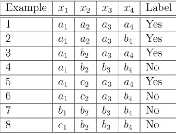
Example x1 x2 x3 x4 Label 1 a1 a2 a3 a4 Yes 2 a1 a2 a3 b4 Yes 3 a1 b2 a3 a4 Yes 4 a1 b2 b3 b4 No 5 a1 c2 a3 a4 Yes 6 a1 c2 a3 b4 No 7 b1 b2 b3 b4 No 8 c1 b2 b3 b4 No
Table 2.1: Data examples used for the decision tree algorithm Fig. 2.7.
The decision tree can then be constructed top-down using the information gain I in the following way:
1. Begin at the root node.
2. Determine the feature with the highest information gain which is not already used as an ancestor node.
3. Add a child node for each possible value of that feature.
4. Attach all examples to the child node where the feature values of the examples are identical to the feature value attached to the node. 5. If all examples attached to the child node can be classified uniquely, add
that classification to that node and mark it as leaf node.
6. Go back to step two if there are unused features left, otherwise add the classification of most of the examples attached to the child node. Fig.2.7shows an example of a decision tree for the training-set of Table2.1. Each of the eight rows in the table represents an example that is described by four features x1, x2, x3, x4 with different values. The last column shows the
labels of each example.
For instance, using the decision tree depicted in Fig. 2.7, the example (x1 = a1, x2 = b2, x3 = a3, x4 = b4) would sort to the nodes: x1, x2, and
finally x3, which would classify the example as being "Yes".
Decision tree algorithms can be implemented serially or in parallel depend-ing upon the size of data set. Some of them such as SLIQ, SPRINT, CLOUDS, BOAT and Rainforest have the capability of parallel implementation. IDE 3, CART, C4.5 and C5.0 are serial classifiers. Haider et al. provided an overview
Figure 2.7: Decision tree applied to data of table 2.1.
of these decision tree algorithms and compared them against pre-defined cri-teria including data dimensionality and root selection metric. The authors concluded that SLIQ and SPRINT are suitable for larger data sets whereas C4.5 and C5.0 are best suited for smaller data sets [Haider 2013].
2.3.3
Perceptron based classifiers
2.3.3.1 Single layered perceptron
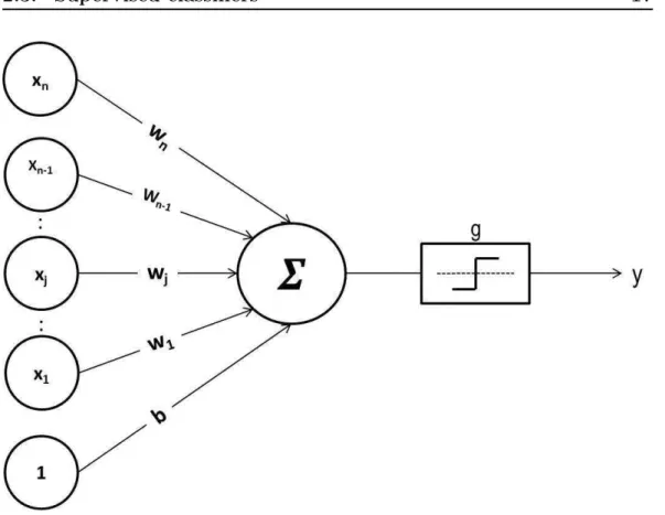
In 1943, McCulloch and Pitts [McCulloch 1943] proposed a binary thresh-old unit as a computational model for a single layered perceptron (Fig. 2.8). Given a data example x, if x1, ...xn are its input feature values and w1, ...wn
are connection weights (typically real numbers in the interval [−1, 1]), then perceptron computes the sum of weighted input units and generates an out-put unit y of 1 if the sum is above a certain threshold b and 0 otherwise. Mathematically: y = g( n ∑ j=1 wjxj− b) (2.10)
Figure 2.8: Single layered perceptron.
where g(.) is a step function at 0. For simplicity of notation, the threshold b is often considered as being another weight w0 =−b attached with a constant
input unit x = 1.
The McCulloch-Pitts perceptron has been generalized in many ways. An obvious way is to use activation functions other than the threshold function. Different types of activation functions are then used depending on the problem at hand. Some examples are given bellow:
• Sigmoidal activation function: g(x) = 1
1+e−βx (β is the slope parameter)
• Hyperbolic tangent activation function: g(x) = e2x−1 e2x+1
• Linear activation function: g(x) = x
• Sinusoidal activation function: g(x) = sin(x)
The training algorithm begins with initial values for the weights w, and iteratively updates these weights until all data examples have been classified correctly or if the iteration number has reached a predefined maximum value.
Figure 2.9: Artificial neural network.
2.3.3.2 Artificial Neural Network
Unfortunately, single layered perceptrons can only classify linearly separable sets of examples. In order to process non-linear cases as well, single lay-ered perceptrons are connected to construct a network called artificial neural network (ANN) (Fig. 2.9. The most commonly used architecture is the Feed-forward network in which the signals are allowed to travel one way only from an input layer to an output layer through one or more hidden layers. The input layer receives the information to be processed (the feature vectors) and in the output layer, the results of the processing are found. Every unit in the input layer sends its activation value (using the equation 2.10) to each of the hidden units to which it is connected. Each of these hidden units calculates its own activation value and the resulted signal is then passed on to the output units.
There are several algorithms with which a network can be trained
[Neocleous 2002]. However, the most well-known and widely used learning
algorithm to estimate the values of the weights is the Back Propagation (BP) algorithm [Russell 2003]. Generally, the BP algorithm includes the following six steps:
1. Present a training example to the neural network and initialize the cor-responding weights.
2. Compare the network’s output to the desired output from that example. Calculate the error in each output neuron.
3. Calculate for each neuron, the local error that represents how much lower or higher the output must be adjusted to match the desired output. 4. Adjust the weights of each neuron to lower the local error.
5. Assign responsibility for the local error to neurons at the previous level, giving greater responsibility to neurons connected by stronger weights. 6. Repeat the above steps with the neurons at the previous level, using
each one’s responsibility as its error.
The BP algorithm will have to perform a high number of weight modifi-cations before it reaches a good weight configuration. Therefore, ANNs use different stopping rules to control when training ends such as stopping after a specified number of epochs or when an error measure reaches a threshold, etc.
The major problem encountered with the ANNs is that they are too slow for most applications. Other approaches are used to speed up the training rate such as Weight-elimination algorithm, Genetic algorithms and Bayesian methods [Willis 1997, Dunson 2005].
2.3.4
Statistical based classifiers
Conversely to perceptron based techniques, statistical approaches are char-acterized by having an explicit underlying probability model, which provides a probability that an instance belongs to each class, rather than simply a classification. Naive Bayes classifiers and Fisher’s linear discriminant (FLD) are popular methods used in statistics and ML to find the linear combina-tion of features which best separate two or more classes. We will give a brief description of each of them.
2.3.4.1 Naive Bayes classifiers
The Naive Bayes classifier is a traditional demonstration of how genera-tive assumptions and parameter estimations simplify the learning process
[Domingos 1997]. Consider the problem of predicting a label y ∈ [0, 1] based
on a vector of features x = (x1, ..., xn), where each xi is assumed to be in [0, 1]
hBayes(x) = argmin y∈[0,1]
P [Y = y|X = x] (2.11)
The number of parameters required to describe the probability density P [Y = y|X = x] is in the order of 2n. This implies that the number of
examples needed grows exponentially with the number of features.
In the Naive Bayes approach a (rather naive) generative assumption is made. This assumption states that given the label, the features are indepen-dent of each other. Mathematically,
P [X = x|Y = y] =
n
∏
i=1
P [Xi = xi|Y = y] (2.12)
The assumption of independence of features is almost always wrong and for this reason, naive Bayes classifiers are usually less accurate than other more sophisticated learning algorithms. Nevertheless, naive Bayes classifier has a major advantage to require a short computational time for training.
Under the assumption of independence and using Bayes rule, the Bayes optimal classifier can be further simplified:
hBayes(x) = argmin y∈[0,1] P [Y = y]P [X = x|Y = y] = argmin y∈[0,1] P [Y = y] n ∏ i=1 P [Xi = xi|Y = y] (2.13)
As a result, the generative assumption reduced significantly the number of parameters from 2n to 2n + 1 only.
2.3.4.2 Fisher’s Linear discriminant
Fisher’s Linear discriminant (FLD) is another demonstration of how genera-tive assumptions simplify the learning process [Fisher 1936]. As in the Naive Bayes classifier, the problem of predicting a label y ∈ [0, 1] based on a vector of features x = (x1, ..., xn) is considered. The generative assumption assumes
first that P [Y = 1] = P [Y = 0] = 1/2 and second, the conditional probability of x given y is a Gaussian distribution such that its covariance matrix is the same for both values of y. Formally, let µ0, µ1 ∈ Rn be the means of class
0 and 1 respectively, and let Σ be a covariance matrix. Then, the density distribution is given by:
P [X = x|Y = y] = 1 (2π)n/2|Σ|1/2 exp [− 1 2(x− µy) TΣ−1(x − µy)] (2.14)
Under this assumption, the Bayes optimal solution is to predict points as being from the second class if the log of what is called the likelihood ratio is below some threshold t:
hBayes(x) =
{
1, if log(P [Y =1]P [X=x|Y =1]P [Y =0]P [X=x|Y =0]) > t
0, otherwise. (2.15)
With the other generative assumptions, the log-likelihood ratio becomes: 1 2(x− µ0) TΣ−1(x − µ0)− 1 2(x− µ1) TΣ−1(x − µ1) (2.16)
which can be rewritten as w· x + b where:
w = (µ1− µ0)TΣ−1 (2.17) and, b = 1 2(µ T 0Σ−1µ0− µT1Σ−1µ1) (2.18)
As a result, the above derivation shows that under the aforementioned generative assumptions, the Bayes optimal classifier is a linear classifier. One may train the classifier by estimating the parameters µ0, µ1 and Σ from the
data, using for example the Maximum Likelihood Estimator (MLE). With those estimators at hand, the values of w and b can be calculated as in Eqs.
2.17 and 2.18.
2.3.5
Support Vector Machines
The Support Vector Machine classifier (SVM) is a supervised learning method belonging to a family of generalized linear classifiers. For binary classification, the main aim is to simultaneously minimize the empirical classification error and maximize the geometric margin between the two-classes. Hence they are also known as maximum margin classifiers. The SVM problem can be reduced to find the hyperplane that maximizes the distance from it to the nearest examples in each class. Since this thesis deals with the application of SVM classifiers to real-world problems, we will devote a part of the next chapter to detail the mathematical basis of linear and non linear SVM classifiers.
2.4
Data processing
In order to gain in generalization performance; regardless the ML algorithm to use; much care should be taken to data processing before training. This may include mainly data balancing and reducing dimensionality.
2.4.1
Data-set balance
Let m+and m−be the number of positive and negative examples respectively.
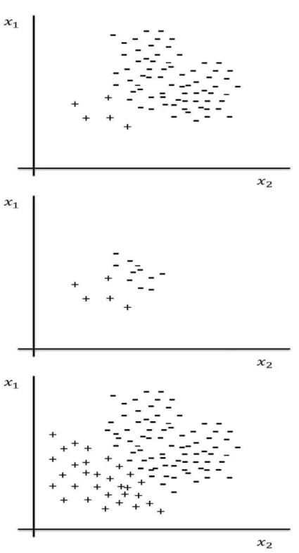
The data-set unbalance problem occurs when the data-set is dominated by positive examples (m+ >> m−). For example, the top graph in Fig. 2.10
shows more negative (-) than positive (+) signs while in the other graphs there is a better balance between the two sets which make it easier to classify. When faced with unbalanced data-sets, the generalization performance of a classifier drops significantly [Akbani 2004].
A data preprocessing method for dealing with unbalanced data falls into one of the following three categories: under-sampling the majority class, over-sampling the minority class, or hybrid of over-over-sampling and under-over-sampling. Examples of each of these methods are given below.
2.4.1.1 Over-sampling methods
- Random Over-sampling (RandOver): This method randomly select ex-amples from the minority class with replacement until the number of selected examples plus the original examples of the minority class is identical to that of the majority class.
- Synthetic Minority class Over-sampling (SMOTE): This method is performed by taking each minority class example and introducing synthetic examples along the line segments joining any/all of the randomly chosen k nearest neighbors of this minority class example [Chawla 2002]. For instance, if the amount of over-sampling needed is 200%, only two neighbors are chosen and one sample is generated in the direction of each. Synthetic examples are generated as follows:
1. Take the difference between the example under consideration and its nearest neighbor;
2. Multiply this difference by a random number between 0 and 1;
3. Add the resulting example to the feature vector under consideration. This causes the selection of a random point along the line segment be-tween two specific examples.
- Agglomerative Hierarchical Clustering (AHC): This method was first used by Cohen et al. [Cohen 2006]. It involves three major steps:
1. Use an agglomerative hierarchical clustering algorithm such as single linkage to form a dendrogram;
Figure 2.10: Data-set unbalance illustration. Top, negative data far outnumber the positive data. Middle, under-sampling the negative data. Bottom, over-sampling the positive data.
2. Gather clusters from all levels of the dendrogram and compute the clus-ter centroids as synthetic examples;
3. Concatenate centroids with the original minority class examples.
2.4.1.2 Under-sampling methods
- Random Under-sampling (RU): This is a non-heuristic method that randomly select examples from the majority class for removal without re-placement until the remaining number of examples is same as that of the minority class. Generally, such a solution leads to lose of information and becomes difficult to accept especially when only very limited amount of data is available [Akbani 2004].
- Bootstrap Under-sampling (BU): This method is similar to RU, but with replacement. An example can be selected more than once.
- Condensed Nearest Neighbor (CNN): This method first randomly draw one example from the majority class to be combined with all examples from the minority class to form a training-set D, then use a 1-NN to classify the examples in this training-set and remove every misclassified example from the training-set to D [Hart 1968].
- Edited Nearest Neighbor (ENN): This method was originally pro-posed by Wilson [Wilson 1972] . It works by removing noisy examples from the original set. An example is deleted if it is incorrectly classified by its k-nearest neighbors.
- Neighborhood Cleaning Rule (NCR): This method was origi-nally proposed by Laurikkala [Laurikkala 2001] and it employs the Wilsons ENN Rule to remove selected majority class examples. For each example Ei = (xi, yi) in the training set, its three nearest neighbors are found. If Ei
belongs to the majority class and the classification given by its three near-est neighbors is the minority class, then Ei is removed. If Ei belongs to the
minority class and its three nearest neighbors misclassify it, then remove the nearest neighbors that belong to the majority class.
- K-Means Based (KM): This method, first used by Cohen et al.
[Cohen 2006]. It applies the k-means clustering algorithm to group the
ma-jority class into sub-clusters and the resulting prototypes of sub-clusters are used as synthetic cases to replace all the original majority class examples.
- Fuzzy-C-Means Based (FCM): This method is similar to KM, except that the fuzzy c-means algorithm is used instead of the k-means clustering algorithm.
2.4.1.3 Hybrid methods
- SMOTE-RU Hybrid: After over-sampling the minority class with SMOTE, the majority class is under-sampled by removing samples randomly from the majority class. The process continue until the minority class reaches a certain percentage of the majority class [Chawla 2002].
- SMOTE-ENN Hybrid: This method uses SMOTE to generate syn-thetic minority examples and then applies ENN to remove each major-ity/minority class example from the data set that does not have at least two of its three nearest neighbors of the same class [Batista 2004].
- AHC-KM Hybrid: This method combines AHC-based over-sampling and KM-based under-sampling [Cohen 2006].
- SMOTE-Bootstrap Hybrid (SMOTE-BU): This method was first proposed by Chawla [Chawla 2002]. It uses SMOTE for over-sampling the minority class followed by Bootstrap sampling the majority class so that both classes have the same or similar number of examples.
2.4.2
Dimensionality reduction
2.4.2.1 The curse of dimensionality
The "curse of dimensionality" is a term coined by Richard Bellman
[Bellman 1961] when dealing with the problem of rapid increase in volume
caused by adding extra dimensions to the feature space. It is a significant obstacle in high dimension data analysis due to the fact that the sparsity increases exponentially given a fixed amount of data points.
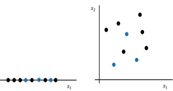
An illustration of this phenomenon is shown in Fig. 2.11 where a 1-NN classifier is used to classify nine examples. On one hand, if one feature, say, x1 is only used (left), obviously, the 1-NN classifier will not be discriminative,
the number of examples seems to be large. On the other hand, with two features, say, x1 and x2 (right), the nine examples will be too sparse and the
1-NN classifier would need more examples to perform well.
In ML problems that involve learning from a finite number of data ex-amples m in a high-dimensional feature space (n features) with each feature having a number of possible values, an enormous amount of training data are required (typically m >> n) to ensure that there are several examples with each combination of values. When one uses machine learning where high di-mensional data (n > m) is involved, one may be faced with drawbacks includ-ing: (1) computational efficiency challenge; (2) poor generalization abilities of the learning algorithm (see section 2.5) and (3) difficulty in interpreting, finding meaningful structure or illustrating the data.
Figure 2.11: Curse of dimensionality. In left, data are in one dimension. In right, data are in two dimensions. The sparsity of data increases with the increase in dimension.
In order to avoid the curse of dimensionality, one can pre-process the data-set by reducing its dimension before running a learning algorithm. One can suspect that there is only a small set of features (let say k features) that are "relevant" to the learning task. The question is, how that set of features can be found? Two solutions are possible:
• selecting smaller feature-subset from the high dimensional set of fea-tures.
• combining the high dimensional set of features to get a smaller feature-set.
2.4.2.2 Feature selection
Most of the methods for dealing with high dimensionality focus on feature selection techniques. The selection of the subset can be done manually by using prior knowledge to identify irrelevant features or by using proper algorithms. Generally, researchers make distinction between two feature selection approaches: wrapper approaches and filtering approaches.
Wrapper approaches
Wrapper approaches wrap around the learning model, and repeatedly make calls to it to evaluate how well it does using different feature subsets.
forward search is one instantiation of wrapper feature selection approaches. It is based on the following steps:
1. Initialize the feature-subset F to be ∅ (F = ∅). 2. Repeat
(a) For i = {1..., n} if i /∈ F, let Fi = F ∪ {i}, and evaluate features
Fi. (I.e., train the learning algorithm using only the features in Fi,
and estimate its generalization error.)
(b) Set Fi to be the best feature subset found on step (a).
3. Select and output the best feature subset that was evaluated during the entire search procedure.
The outer loop of the algorithm can be terminated either when F = {1, ...n} is the set of all features, or when |F| exceeds some pre-set thresh-old k corresponding to the maximum number of features that one want the algorithm to consider using.
Beside forward search, other search procedures can also be used. For example, backward search starts off with F = {1, ...n} as the set of all features, and repeatedly deletes features one at a time (evaluating feature deletions in a similar manner to how forward search evaluates single-feature additions) untilF = ∅.
Wrapper feature selection algorithms often work quite well, yet, it is com-putationally costly according to the need to make many calls to the learning algorithm. Indeed, exhaustive forward or backward search would take about O(n2) calls to the learning algorithm.
One of the well known wrapper methods is the support vector machine based recursive feature elimination (SVM-RFE) algorithm. It will be detailed in section 3.5 of chapter 3.
Filtering approaches
Filtering approaches give heuristic, but computationally much cheaper, ways of choosing a feature subset. The idea here is to compute some simple score S(i) that measures how informative each feature xi is about the class
labels y. Then, simply pick the k features with the largest scores S(i). One possible choice of the score would be define S(i) to be (the absolute value of) the correlation between xi and y, as measured on the training-set. This would
the class labels. In practice, it is more common (particularly for discrete-valued features xi) to choose S(i) to be the mutual information between xi
and y. If xi and y are independent, then xi is clearly very non-informative
about y, and thus the score S(i) should be small. Conversely, if xi is very
informative about y, then S(i) would be large.
Filtering approaches are very efficient and fast to compute, however, a feature that is not useful by itself can be very useful when combined with others.
2.4.2.3 Features combination
Rather than eliminating irrelevant and redundant features, other methods are concerned with transforming the observed features into a small number of "projections" or "dimensions". The underlying assumptions are that the features are numeric and the dimensions can be expressed as linear combinations of the observed features (and vice versa). Each discovered dimension is assumed to represent an unobserved factor and thus to provide a new way of understanding the data. A number of algorithms dealing with the linear dimensionality reduction have been developed over the years [ref]. One of the most popular is the principal components analysis (PCA).
Principal components analysis (PCA)
With principal components analysis, the dimensionality reduction is performed by highlighting the similarities and differences in the data-set
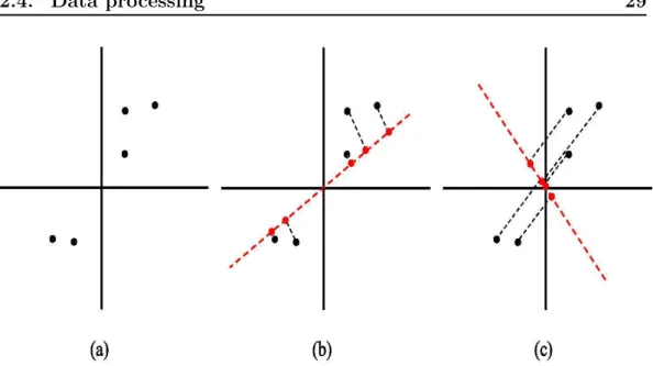
[Jolliffe 2002]. For example, consider the data-set (dark circles) in Fig. 2.12
and suppose we want to reduce dimensionality of this data-set from 2-dimensions to 1-dimension. One should first normalize the data so that the features have zero mean µ and unit variance σ. This ensures that different features could be treated in the same scale. The normalization steps are as follows:
1. Let µj = m1 ∑mi=1xj(i)
2. Replace each xj(i) with xj(i)− µi
3. Let σj2 = m1 ∑mi=1(xj(i))2
4. Replace each xj(i) with xj(i)/σj
PCA attempts to find a direction u(1) ∈ IRn onto which to project the
Figure 2.12: Principal component analysis. (a) original normalized data in two dimension. (b) first projection. (c) second projection. PCA attempts to find the projection that maximize the variance of the projected data (b).
distances). In other words, PCA attempts to maximize the variance of the projected data (the red circles).
Suppose we pick two directions (dashed red lines), we see that the projected data have a fairly large variance in Fig.2.12(b) and tend to be far from zero. In contrast, in Fig.2.12(c) the projections have a significantly smaller variance, and are much closer to the origin.
In general, to reduce the dimensionality from n-dimensions to k-dimensions, PCA attempts to find k vector u(1), u(1), ...u(k) ∈ IRn onto which
to project the data so as to minimize the projection error.
To formalize this, let consider a unit vector u and a data point x(i), the
distance from the origin of the projection of x(i) onto u is given by x(i)Tu.
Hence, to maximize the variance of the projections, one would like to choose a unit-length u so as to maximize the expression:
1 m m ∑ i=1 (x(i)Tu)2 = uTΣu (2.19) with: Σ = m ∑ i=1 x(i)x(i)T (2.20)
Σ is just the empirical covariance matrix of the data assumed to have zero mean.
To summarize, in order to find a 1-dimensional subspace to approximate the data, u must be the principal eigenvector of Σ. More generally, to project data into a k-dimensional subspace (k < n), one should choose u1, ..., uk to
be the k eigenvectors corresponding to the highest eigenvalues of Σ . The ui’s
now form a new, orthogonal basis for the data (since Σ is symmetric). Then, to represent x(i) in this basis, one only needs to compute the corresponding
vector: y(i) = u1Tx(i) u2Tx(i) .. . ukTx(i) ∈ IRk
Thus, whereas x(i) ∈ IRn, the vector y(i) now gives a lower, k-dimensional,
representation for x(i). The vectors u
1, ..., uk are called the first k principal
components of the data.
2.5
Model selection
In supervised learning, a model must be selected from among a set of models. By selecting a model, we mean finding the optimal parameters with which a model can "explain well" the training-set, but also "generalize well" to new unseen examples. One can therefore make distinction of three possible config-urations: In the first one, the model "does not explains well" the training-set and in this case it will do "very bad" on new examples. In other words, this model has a high bias or is underfitting the training-set. In the second con-figuration, the model "explains well" the training-set and is "good enough" when predicting new examples. In the third configuration, the model "ex-plains very well" the training-set but is "very bad" on new examples. In this last configuration, one say that the model has high variance or is overfitting the training-set.
Intuitively, the second configuration seems to be preferred and selecting a model will be reduced to finding the one that is just right in the bias-variance tradeoff.
2.5.1
Example of bias-variance tradeoff
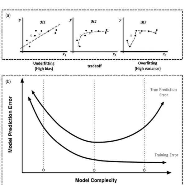
Let’s consider the data in the scatter plots of Fig. 2.13(a). The filled circles represent the training-set and the the not filled circles represent the test-set. The gray curves attempt to model the training-set using three polynomial regression models:
• M2: y = a + bx1+ cx12.
• M3: y = a + bx1+ cx12+ dx13+ ex14+ f x15+ gx16
At very low levels of complexity (M1), the model seems too simple for the
training-set and consequently it does not fit well the test-set. This is the case of high bias (or underfitting).
Very high level of complexity (M3) helps fitting the training-set but it
causes the model to do a worse job of predicting the test-set. Consequently, we say that the complex model has a high variance or is overfitting the training-set.
Clearly what we want is a model which is powerful enough to represent the underlying structure of the training-set, but not so powerful that it faithfully models the test-set. In other words, a model that is just right in the bias-variance tradeoff (M2).
2.5.2
Cross Validation
One way to find the optimal model parameters is the use of cross validation where the data is split into two sets: a training-set and a validation-set. The idea is to choose the model in which the error of the validation-set is minimum. This is illustrated in the Fig. 2.13(b). Let the true prediction error be the number of classification errors made on validation-set divided by the number of examples in validation-set and let the training error be the number of classification errors made on training-set divided by the number of examples in training-set. The training error decreases as the model complexity grows while the true prediction error decreases until a certain level of complexity before rising up. At that level of complexity, the model is just right in the bias-variance tradeoff.
Splitting data to perform cross-validation is a critical issue. On one hand, training involving as many examples as possible may lead to better models. However, having a small validation-set means that the validation-set may fit well, or not fit well, just by luck. On the other hand, the computed errors will depend on the chosen way in splitting data. There are various methods that have been used to reuse examples for both training and validation in order to improve the generalization error [Kohavi 1995, Lemm 2011, Hastie 2009].
In the so called k-fold cross-validation, data are divided into k mutually exclusive and exhaustive equal-sized subsets: D1, ..., Dk. For each validation
subset, Di, one should train on the union of all of the other subsets, and
empirically determine the prediction error, εi, on Di. An estimate of the
prediction error that can be expected on new examples of a model, trained on all the examples in data, is then the average of all εi’s.
Figure 2.13: Bias-variance tradeoff. (a) The gray curves attempts to model the training-set (filled circles) using three polynomial regression models. The modelM1
has high bias, the model M3 has high variance and the model M2 is just right in
the bias-variance tradeoff. (b) Cross-validation. At each level of complexity, the training error and the true prediction error are computed using different training and validation sets. In the case of high bias, both the training error and the true prediction error have high values. In the case of high variance, the training error is very low but the true prediction error is very high. Using cross-validation, one can find the model allowing the bias-variance tradeoff.
Leave-one-out cross validation (LOO-CV) is the same as cross validation for the special case in which k = m, m being the number of examples, and each Di consists of a single example. When validating on each Di, one simply note
whether or not a mistake was made. The total number of mistakes divided by k yield the estimated prediction error. This type of validation is, of course, more expensive computationally, but useful when a more accurate estimate of the error rate for a classifier is needed.
It is worth mentioning that the validation-set used as part of training is not the same as the test-set. The test-set is used to evaluate how well the learning algorithm works as a whole. So, it is cheating to use the test-set as part of learning since the aim is to predict unseen examples.
2.6
Classifier performance evaluation
2.6.1
Accuracy metric
ML algorithms come with several parameters that can modify their behaviors and performances. Evaluation of a learned model is traditionally performed by maximizing an accuracy metric. Considering a basic two-class classification problem, let {p, n} be the true positive and negative class labels and {Y, N} be the predicted positive and negative class labels. Then, a representation of classification performance can be formulated by a confusion matrix (contin-gency table), as illustrated in Fig. 2.14. Given a classifier and an example, there are four possible outcomes. If the example is positive and it is classified as positive, it is counted as a true positive (TP); if it is classified as negative, it is counted as a false negative (FN). If the example is negative and it is classified as negative, it is counted as a true negative (TN); if it is classified as positive, it is counted as a false positive (FP). Following this convention, the accuracy metric is defined as:
Acc = T P + T N
m++ m− (2.21)
where m+ and m− are the number of positive and negative examples
re-spectively (m+ = T P + F N, m−= F P + T N ).
However, accuracy can be deceiving in certain situations and is highly sensitive to changes in data. In other words, in the presence of unbalanced data-sets (i.e., where m+ >> m−), it becomes difficult to make relative
Figure 2.14: Confusion matrix.
2.6.2
Receiver Operating Characteristic (ROC) Curve
Metrics extracted from the receiver operating characteristic (ROC) curve can be a good alternative for model evaluation, because they allow the dissociation of errors on positive or negative examples. The ROC curve is formed by plotting true positive rate (TPR) over false positive rate (FPR) defined both from the confusion matrix by:
T P R = T P
m+ (2.22)
F P R = F P
m− (2.23)
Any point (F P R; T P R) in ROC space corresponds to the performance of a single classifier for a given distribution. The ROC space is useful because it provides a visual representation of the relative trade-offs between the benefits (reflected by T P ) and costs (reflected by F P ) of classification in regards to data distributions.
Generally, the classifier’s output is a continuous numeric value. The de-cision rule is performed by selecting a dede-cision threshold which separates the positive and negative classes. Most of the time, this threshold is set regard-less of the class distribution of the data. However, given that the optimal threshold for a class distribution may vary over a large range of values, a pair (FPR;TPR) is thus obtained at each threshold value. Hence, by varying this threshold value, a ROC curve is produced.
Fig. 2.15 illustrates a typical ROC graph with points A, B and C rep-resenting ROC points and curves L1 and L2 reprep-resenting ROC curves. Ac-cording to the structure of the ROC graph, point A (0,1) represents a perfect classification. Generally speaking, one classifier is better than another if its corresponding point in ROC space is closer to the upper left hand corner. Any