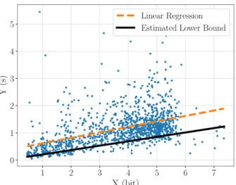
Regression to a Linear Lower Bound With Outliers: An Exponentially Modified Gaussian Noise Model

Outline. The article proceeds as follows: we introduce the optimization problem coming from the classical SVR and describe the modifications brought by adding linear constraints

In a fully Bayesian treatment of the probabilistic regression model, in order to make a rigorous prediction for a new data point, it requires us to integrate the posterior

We see that CorReg , used as a pre-treatment, provides similar prediction accuracy as the three variable selection methods (this prediction is often better for small datasets) but

Keywords: linear regression, Bayesian inference, generalized least-squares, ridge regression, LASSO, model selection criterion,

Focusing on a uniform multiplicative noise, we construct a linear wavelet estimator that attains a fast rate of convergence.. Then some extensions of the estimator are presented, with

In this paper, we consider an unknown functional estimation problem in a general nonparametric regression model with the feature of having both multi- plicative and additive

Our approach is close to the general model selection method pro- posed in Fourdrinier and Pergamenshchikov (2007) for discrete time models with spherically symmetric errors which

1) Center model: This model (also called CM method) was first proposed by Billard and Diday [18]. In this model only the midpoints of the intervals are considered to fitting a