HAL Id: inria-00576479
https://hal.inria.fr/inria-00576479
Submitted on 15 Mar 2011
HAL is a multi-disciplinary open access
archive for the deposit and dissemination of
sci-entific research documents, whether they are
pub-lished or not. The documents may come from
teaching and research institutions in France or
L’archive ouverte pluridisciplinaire HAL, est
destinée au dépôt et à la diffusion de documents
scientifiques de niveau recherche, publiés ou non,
émanant des établissements d’enseignement et de
recherche français ou étrangers, des laboratoires
Local regularity-based interpolation
Pierrick Legrand, Jacques Lévy Véhel
To cite this version:
Pierrick Legrand, Jacques Lévy Véhel. Local regularity-based interpolation. WAVELET X, Part of
SPIE’s Symposium on Optical Science and Technology, SPIE, Aug 2003, San Diego, United States.
�inria-00576479�
Local regularity-based interpolation
Pierrick Legrand, Jacques L´evy V´ehel Projet Fractales, IRCCyN
1 Rue de la No´e, B.P. , 44000 Nantes, France {Pierrick.Legrand, Jacques.Levy-Vehel}@irccyn.ec-nantes.fr
Description of the work and motivation
A ubiquitous problem in signal processing is to obtain data sampled with the best possible resolution. At the acquisition step, the resolution is limited by various factors such as the physical properties of the captors or the cost. It is therefore desirable to seek methods which would allow to increase the resolution after acquisition. This is useful for instance in medical imaging or target recog-nition. In some applications, one dispose of several low resolution overlapping signals [1]. In more general situations, a single signal is available for superres-olution. Interpolation then requires that the available data be supplemented by some a priori information. Two types of methods have been explored: In the first, ”class-based” one, the signal is assumed to belong to some class, with conditions expressed mainly in the time or frequency domain [3, 5, 10]. This puts constraints on the interpolation, which is usually obtained as the mini-mum of a cost-function. The second type of approaches hypothesizes that the information needed to improve the resolution is local and is present in a class of similar signals [2, 4]. This type of approach could be called ”contextual”. Both ”class-based” and ”contextual” approaches use a ”model” for interpola-tion: The ”class-based model” is that the signal belongs to an abstract class characterized by a certain mathematical property. The ”contextual model” is that the signal will behave locally under a change of resolution in way ”similar” to other signals in a given set, for which a high resolution version is known. Both types of techniques have some drawbacks. Roughly speaking, class-based methods generally lead to overly smooth signals, while contextual-based ones, on the contrary, tend to generate spurious details.
Our motivation is to find a way to interpolate in such a way that smooth regions as well as irregular ones (e.g. sharp edges) remain so after zooming. We interpret this as the constraint that interpolation should preserve the local regu-larity. We measure this regularity through a notion of H¨older exponent. H¨older exponents have been shown to correspond to an intuitive notion of regularity in both images and 1D signals [6]. In order to control the interpolation and obtain a simple implementation, we need to make some assumptions on the signal, to the effect that (a) this H¨older exponent can be easily estimated from wavelet coefficients (b) the exponent allows to predict the finer scales coefficients. Tech-nically, this requires that the signal is not oscillatory. Our scheme allows to control both the reconstruction error and the regularity of the interpolated sig-nal, i.e. the visual appearance of the added information.
1
The method
The method is best understood in terms of wavelet coefficients: Let X de-noted the input signal and let dj,k be its wavelet coefficients, where, as usual, j
corresponds to scale and k to location. Roughly speaking, if a signal has reg-ularity α at point t, then its wavelet coefficient dj,k(j,t) ”above” t are bounded
by C2−jα for some constant C: ∀j = 1 . . . n, |d
j,k(j,t)| ≤ C2−jα. The
expo-nent α corresponds to an intuitive notion of regularity: A large α translates in a smooth signal, while α ∈ (0, 1) means that the signal is continuous and non differentiable at t. If the signal is discontinuous at t but bounded, then α = 0. Now if we are willing to conserve the regularity, we should prescribe the wavelet coefficient above t at the superresolved scale n + 1 in such a way that |dn+1,k(n+1,t)| ≤ C2−(n+1)α.
For concreteness, let us explain schematically how our method would act on a uniform region and on a step edge. On a uniform region, all the wavelet coefficients are close to zero. The bound on the wavelet coefficients then holds with arbitrarily large α, since 0 ≤ C2−jα for all α > 0. As a consequence, the
predicted coefficient dn+1,kwill be zero, since it must satisfy the same inequality:
Smooth regions will remain smooth, because no detail will be added. On the other hand, above a step edge, the wavelet coefficients dj,kdo not decay in scale.
This imply that α = 0. The predicted coefficient dn+1,kwill then be of the same
order as dn,k. As a consequence, the local regularity of the interpolated image
will be again equal to 0 at this point, and the edge will not be blurred.
Our approach has similarities with both class-based and contextual methods. As in class-based methods, we do not rely on information learnt from a database, and require that the signal belongs to a definite class. A distinctive feature is that our class is based on local features. The similarity with contextual approaches is that the information is learnt from the image instead of being a priori, as in class-based ones. Also, this information is local in space and scale, and is versatile enough to handle a wide variety of situations.
Let X denote the original signal, and Xn= (xn1, . . . xn2n) its regular sampling
over the 2npoints (tn
1, . . . tn2n). Let ψ denote a wavelet such that the set {ψj,k}j,k
forms an orthonormal basis of L2. Let d
j,k be the wavelet coefficients of X.
For p = 1 . . . 2n, we consider the point t = tn
p and the wavelet coefficients
which are located ”above” it, i.e. dj,k(j,t) with k(j, t) = ⌊(t − 1)/(2n+1−j)⌋ + 1.
Let αn(t) denote the slope of the liminf regression (see [7] for an account on
liminf regressions) of the vector (log(d1,k(1,t), . . . dn,k(n,t)) versus (−1, . . . , −n).
When n tends to infinity, αn(t) tends to liminf
log dn,k(n,t)
−n . This number has been
considered in the literature [9] under the name of weak scaling exponent, denoted βw. It is a measure of the local regularity in the following sense. The weak
scaling exponent of the signal X at t0 is defined as: βw= sup{s : ∃n, X(−n)∈
Cts+n0 } where X(−l) denotes a primitive of order l of X and Cs
t0 is the usual
pointwise H¨older space at t0. When the local H¨older exponent αl and the
pointwise H¨older exponent αp of X at t coincide, then βw is also equal to their
assume that this is the case. In other words, we consider that our signals belong to the class S defined as follows:
S = {X ∈ L2(IR), ∀t ∈ IR, αp(t) = αl(t)}
The class S may appear somewhat abstract to the reader. Here are a few clues. S contains all C∞ signals and all signals of the type P
n∈IN|t − tn|γn,
with tn ∈ IR, γn ∈ IR+. Many everywhere irregular signals are also in S, such as
the continuous nowhere differentiable Weierstrass functionPn∈IN2−nhsin(2nt),
h ∈ (0, 1). On the other hand, ”chirp” signals as |t|γsin(1/|t|β), γ > 0, β > 0
do not belong to S. For X in S, at each point t, the ”largest” coefficients are located above t in the following sense. Take any sequence dj,k of coefficients
such that k2−j tends to t. Then, if X belongs to S,
liminfj→∞
log |dj,k|
−j ≥ liminf j→∞
log |dj,k(j,t)|
−j (1)
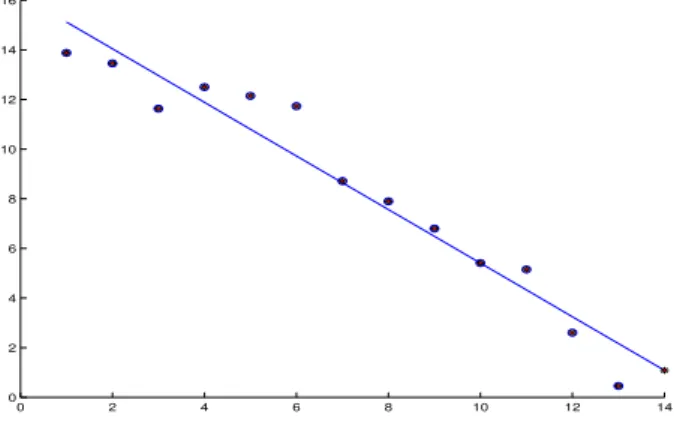
Such signals are called ”non-oscillatory” in the literature. To perform the in-terpolation, we compute above each point t the regression of the wavelet co-efficients vs scale (figure 1). The parameters of the regression allow to build the extrapolated coefficient. These coefficients in turn determine the ”superre-solved” signal. For a sampled signal Xn, we denote ˜Xn the signal interpolated
on infinitely many levels.
2
Regularity and Asymptotic properties
Proposition 1 Let X be in Cη for some η > 0. Then, for all ε > 0, there
exists N such that for all n > N , all p and all t ∈ (tn
p, tnp+1), α ˜ Xn p (t) = α ˜ Xn l (t) ∈ [β − ε, β + ε], where β = min(βw(tnl), βw(tnl+1)).
Proposition 2 Let X belong to S, and assume X ∈ Cα. Then, ∀ε > 0, ∃N :
n > N ⇒ ||X− ˜Xn||2= O(2−n(α−ε)). In addition, ||X− ˜Xn||Bs
p,q = O(2
−n(α−s−ε))
for all s < α − ε.
3
Numerical experiments
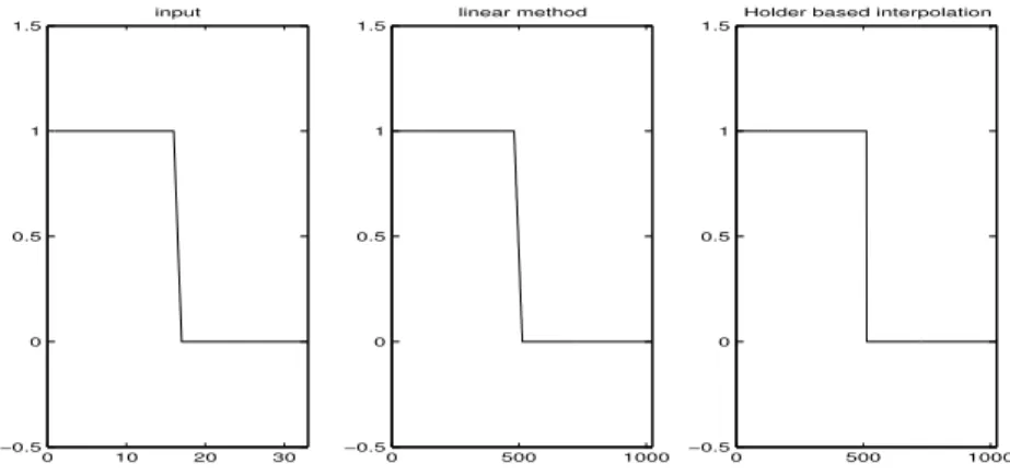
We provide experiments on a step edge (figure 2), a generalized Weierstrass function (figure 3), and a real-world signal, namely a road profile (figure 4). In each case, we compare our method with a simple linear interpolation.
References
[1] S. Baker, T. Kanade, Super-resolution: Reconstruction of Recognition, Proc. of IEEE-Eurasip Workshop on Nonlinear Signal and Image Processing, 2001, pp. 349-385. [2] F.M. Candocia, J.C. Principe, Superresolutions of images based on local correlations,
[3] D. M. Donoho, I. M. Johnstone,J.C. Hoch, A.S. Stern, Maximum Entropy and the Nearly Balck Object, J.R. Statist. Soc. B., 54 1 (1992), pp. 41–81 .
[4] W.T. Freeman, T.R. Jones, E.C. Pazstor, Example-Based Super-Resolution, MERL Tech. Rep. 2001-30, 2001.
[5] K.-L Kueh, T. Olson, D. Rockmore, K.-S Tan, Non-linear Approximation Theory on Finite Group, 1999.
[6] J. L´evy V´ehel, Fractal Approaches in Signal Processing, Fractals, 3(4) (1995), pp. 755-775.
[7] P. Legrand, J. L´evy V´ehel, Signal Processing with FracLab Preprint [8] J. L´evy V´ehel, S. Seuret The 2-microlocal formalism, preprint.
[9] Y. Meyer, Wavelets, Vibrations and Scalings, American Mathematical Society, 9 (1997), CRM Monograph Series.
[10] D.C. Youla, H. Webb, Image restoration by the method of convex projections: Part I - theory, IEEE Tr. Med. Imag. 1(2), 1982, pp. 81–94.
0 2 4 6 8 10 12 14 0 2 4 6 8 10 12 14 16
Figure 1: Regression above a point of the signal. We find scales in abscissa and the log of the wavelet coefficients in ordinate. The extrapolated coefficient is the rightmost point.
0 10 20 30 −0.5 0 0.5 1 1.5 input 0 500 1000 −0.5 0 0.5 1 1.5 linear method 0 500 1000 −0.5 0 0.5 1 1.5
Holder based interpolation
Figure 2: Interpolation of a step edge (32 points to 1024 points). Notice how the edge is not blurred with the H¨older based interpolation.
0 100 200 −2 −1 0 1 2 3 4
Low resolution generalized Weierstrass
0 200 400 −2 −1 0 1 2 3 4 5 linear method 0 200 400 −2 −1 0 1 2 3 4 5
Holder based interpolation
20 40 60 0 0.5 1 1.5 2 Zoom1 460 480 500 −1.2 −1 −0.8 −0.6 −0.4 −0.2 Zoom2 0 200 400 −2 −1 0 1 2 3 4 5
Hight resolution generalized Weierstrass
Figure 3: Generalized Weierstrass (Pn∈IN2−ntsin(2nt)) with zooms and
com-parison with linear interpolation. Notice how the H¨older based method preserves the irregular as well as regular parts of the signal. In the zoomed figures the H¨older based interpolation is the dashed one.
0 50 100 −1.54 −1.52 −1.5 −1.48 −1.46 −1.44 −1.42 −1.4x 10 4 Road profile 0 1000 2000 −1.54 −1.52 −1.5 −1.48 −1.46 −1.44 −1.42 −1.4x 10 4 linear method 0 1000 2000 −1.54 −1.52 −1.5 −1.48 −1.46 −1.44 −1.42 −1.4x 10 4
Holder based interpolation
780 800 820 840 −1.4334 −1.4332 −1.433 −1.4328 −1.4326 −1.4324 x 10⁴ Zoom1 1900 1920 1940 1960 1980 −1.5 −1.498 −1.496 −1.494 −1.492 −1.49 x 10⁴ Zoom2