1
ATTEL PROJECT
PERFORMANCE-BASED APPROACHES FOR HIGH STRENGTH
TUBULAR COLUMNS AND CONNECTIONS UNDER
EARTHQUAKE AND FIRE LOADINGS
Deliverable 3 – Cyclic testing
- D3.1: monotonic and cyclic test data on base-joint specimens; - D3.2: monotonic and cyclic test data on column specimens;
- D3.3: monotonic and cyclic test data on beam-to-column joint specimens; - D3.4: cyclic test results laboratory report.
Contributing Partners: Centro Sviluppo Materiali Stahlbau Pichler University of Thessaly University of Trento
2
TABLE OF CONTENTS
I. Deliverable 3.1 : base joint specimens ... 4
I.1. Column base joint ... 4
I.1.1. Column base joint design for static loading ... 4
I.1.2. Standard joint for seismic loading ... 6
I.1.3. Innovative joint under seismic loading ... 8
I.2. Tests on base plates component ... 11
I.2.1. Experimental procedure-Instrumentation ... 11
I.2.2. Experimental Results ... 12
II. Deliverable 3.2 : column specimens ... 16
II.1. Mechanical characterization of materials ... 17
II.2. Tensile tests ... 17
II.2.1. Cyclic tests ... 18
II.2.2. Residual stresses ... 19
II.2.3. Discussion and conclusions ... 24
II.3. Tests on column specimens ... 24
II.3.1. Geometrical measurements before testing ... 26
II.3.2. Axial compression tests ... 27
II.3.3. Combined axial and bending tests ... 29
III. Deliverable 3.3 : Beam-to-column joint specimens ... 31
III.1. Beam-to-column joints ... 31
III.2. Beam-to-column through-plate component ... 36
III.2.1. Test Instrumentation ... 36
III.2.2. Experimental Results ... 37
III.3. Slab reinforcement component ... 39
III.4. Experimental results on joints ... 46
III.4.1. Types of test ... 46
III.4.2. Column-base joints ... 48
III.4.3. Beam-to-column joint ... 51
III.5. Column full-scale tests data sheets ... 55
III.5.1. As1... 55 III.5.2. As3-13 ... 56 III.5.3. As3-25 ... 56 III.5.4. As3-50 ... 58 III.5.5. As3-75 ... 60 III.5.6. Bs1 ... 62
3 III.5.7. Bs3-13 ... 63 III.5.8. Bs3-25 ... 63 III.5.9. Bs3-50 ... 65 III.5.10. Bs3-75 ... 67 III.5.11. Al1 ... 69 III.5.12. Al3-25 ... 71 III.5.13. Al3-50 ... 72 III.5.14. Al3-75 ... 73 III.5.15. Bl1 ... 74 III.5.16. Bl3-25 ... 75 III.5.17. Bl3-50 ... 76 III.5.18. Bl3-75 ... 77 IV. References ... 78
4
I. Deliverable 3.1 : base joint specimens
I.1.
Column base joint
Tests on joints are essential in order to understand the behaviour of joints and to propose their numerical model. This in order to evaluate the both mechanical and hysteretic response of the whole structure.
In agreement with the prototype structure designed in the WP2 and the aim of the project, three different solutions were tested by the Trento’s Laboratories:
• 2 tests on the base-joint designed for the static solution, considering joint without stiffeners; • 2 tests on the base-joint designed for the seismic solution, considering a fully-rigid and full
strength joint with stiffeners complying the capacity design proposed in EN 1998-1(2005); • 2 tests on the improved base-joint designed for the seismic solution, considering a fully-rigid
and full strength joint with extended columns in the foundations.
In detail each typology of column-base joints was tested under cyclic and random test, as showed below.
Together with the finalisation of the detailing of the joints, the test set-ups weredesigned too. With reference to the base joints, a scheme of the experimental set-up is depicted in theFigure 1.
In detail, preloaded Dywidag bars were used in order both to restrain the foundation and to apply axial load equal about 700 kN in the column;while, the horizontal force is applied by means of electro-hydraulic actuator MTS with stroke equal to ±250mm and maximum load equal to ±1000kN.
Figure 1. Test set-up of column-base joint test at UNITN Laboratory
I.1.1. Column base joint design for static loading
Column base joints were designed for static loadings considering a semi-rigid joint without stiffeners. The specimens were realized in three steps: i) the cast of foundation blocks; ii) the positioning of circular hollow columns exploiting anchor bolts; iii) the cast of the expansive grout. Figure 2 shows the realization of these column-base joints made at the Materials and Structural Testing Laboratory of the University of Trento (UNITN Laboratory).
These werecharacterized by:
• CHS columns realized using 323,9 x 10 tubular columns in HSS S590 steelgrade; • C30/37 concrete;
5
Figure 2. Realization of the column-base joints designed for the static solution at the UNITN Laboratory
In order to better understand the behaviour of each joint, different type of instruments were used during the test. In detail:
• Seika inclinometers, as shown in Figure 3, were used to monitor the flexural deformation of the columns;
• Linear strain gauges, welded on the base plate to evaluate strain and stress on the elements, as depicted in Figure 4.
• LVDT transducers, as shown in Figure 5, were used to monitor the elongation of joint components.
6
Figure 3. Inclinometers position Figure 4. Strain gauges position on base plate
Figure 5. LVDTs position on anchor bolts and base plate
I.1.2. Standard joint for seismic loading
Figure 7 shows a column-base joint designed for seismic loading considering a rigid and full strength joint with stiffeners complying with the capacity design proposed in EN 1998-1 (2005). The specimens were realized in three steps: i) the cast of foundation blockswith the re-bars of the column; ii) the positioning of circular hollow columns exploiting anchor bolts; iii) the filling of the hollow column with concrete.
Thefollowing pictures of Figure 7 show the realization of the column-base joints characterized by: • CFT columns realized using 355,6 x 12 tubular columns in HSS S590 steelgrade;
• C30/37 concrete;
• 8 B450 C rebars inside the column; • 8 M27 anchor bolts, class 8.8;
7
Figure 6. Realization of the column-base joints designed for the standard seismic solution at the UNITN Laboratory
Figure 7. Realization of the column-base joints designed for the standard seismic solution at the UNITN Laboratory
Instruments used during the test are listed herein:
• Seika inclinometers as in tests on column-base joints designed under static load, see Figure 3; • LVDT transducers, as shown inFigure 8, were used to monitor the elongation both of anchor
bolts and of the base plate;
• Linear strain gauges, welded both to the re-bars and to the plate to evaluate strain and stress on the elements, as depicted in Figure 9.
8
Figure 8. LVDTs position on anchor bolts and plate
Figure 9. Strain gauges position on plate and inside the column, on the rebars
I.1.3. Innovative joint under seismic loading
Figure 10 shows the improved column-base joint designed for seismic loading,considering a fully-rigid and full strength joint with columns embedded into thefoundations. This typology of joint required more attention in the location of thereinforced bars owing to the large number or reinforced bar employed. Three stepswere required in order to realize these joints: i) filling of the hollow circular columnswith re-bars; ii) casting of the foundation blocks with instrumented re-bars andrealization of appropriate holes in order to insert the columns; iii) correct positioningthrough anchor bolts of the columns in the holes and filling of the free space withexpansive grout.
Figure 10 shows the realization of the relevant base joints characterized by:
• CFT columns realized using 355,6 x 12 tubular columns in HSS S590 steel grade; • C30/37 concrete;
• 8 B450 C re-bars inside the column; • 4 M27 anchor bolts class 8.8;
9
Figure 10. Realization of the column-base joints designed for the innovative seismic solution at the UNITN Laboratory
Instruments used during testing are listed here:
• Seika inclinometers as in tests on column-base joints designed under static load, see Figure 3; • LVDT transducers, as shown in Figure 11, were used to monitor the elongation both of anchor
bolts and of the base plate;
• Linear strain gauges, welded both to the re-bars and to the plate to evaluate strain and stress on the elements, see Figure 12;
• Linear strain gauges were positioned on the re-bars in the concrete foundations in order to take into account the activation of the strut&tie mechanisms as shown in Figure 13.
10
Figure 11. LVDTs position on anchor bolts and plate
Figure 12. Strain gauges position on plate and inside the column, on the re-bars
11
I.2.
Tests on base plates component
This experimental investigation consists of three (3) base plate tests (denoted as Component 3) to determine the flexural response of the rectangular base steel plate of a tubular column. The specimens have been subjected to a monotonic pure bending moment. Three (3) plate thicknesses were examined, that is tpl=14, 16 and 18 mm. The steel tubes are made of high-strength steel (TS590) with a nominal
yield stress of 735 MPa and the base plates of S355 steel. The nominal cross-section for the tubes is CHS 193.7x10. The high-strength tubes have been produced by Tenaris Dalmine, and the specimens segments were manufactured by Stahlbau Pichler.
I.2.1. Experimental procedure-Instrumentation
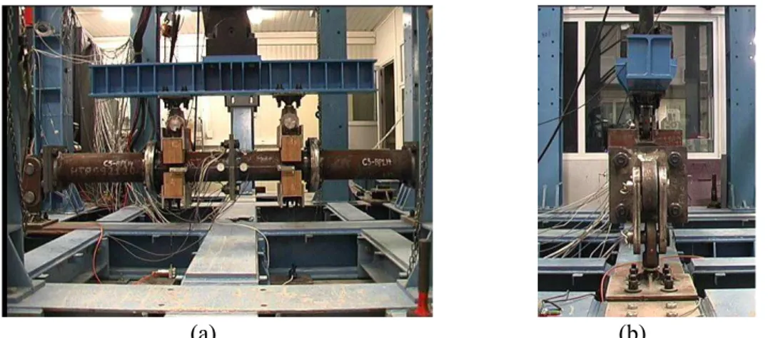
The dimensions of the steel plates are 400x400 mm and they are connected with four (4) M30 bolts, as shown in Figure 14. For the Component 3 tests, 4-point bending was applied to the tubular section of the specimens through a steel cross-beam with two special ball-joint hinges and appropriate wooden grip assemblies. Both ends of the specimens were supported by a double-hinge ‘roller’ system.
(a) (b)
Figure 14. Test setup for the Component 3 tests: (a) front view and (b) side view with double-hinge ‘roller’ system.
The instrumentation setup consisted of wire position transducers and DCDT’s for measuring load-point and support displacements, respectively, and inclinometers for measuring rotation of the tubes relative to the base (see Figure 15a). Strain gages were placed on the base plates at a distance of 25 mm to measure longitudinal and transverse strains starting at 5 mm away from the weld- toe (see Figure 15b). The base plate instrumentation is shown in Figure 16.
(a) (b)
Figure 15. Component 3 base plate instrumentation measuring: (a) base rotation, (b) strain along lines A, B and C.
A
B
12
Figure 16. Strain gage instrumentation for base plate.
I.2.2. Experimental Results
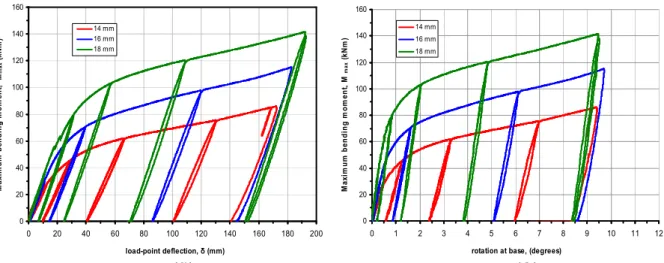
The specimens were subjected to monotonic 4-point bending loading with a stroke rate of 0.1 mm/sec. Three representative load-point displacements values of 90, 100 and 120 mm and corresponding base rotation values of 4, 5 and 6 deg. from the experimental results were chosen to describe flexural behavior of the specimens in the yielding region. The measured experimental results are presented in Table 1.
Table 1. Test results for Component 3 specimens.
type of specimen base plate thickness, tpl (mm)
applied moment, Mmax (kNm)
at load-point deflection of
applied moment, Mmax
(kNm) at base rotation δ=90 mm δ=100 mm δ=120 mm r=4 o r=5o r=6o Component 3 14 67.3 69.4 73.5 64.8 68.7 72.2 16 89.8 92.7 96.6 87.5 92.7 97.3 18 115.4 118.2 122.9 116.5 120.9 125.4
The specimen with a plate thickness of tpl=14 mm resisted a bending moment of 67.3 kNm at a
load-point displacement of δ =90 mm, a bending moment of 69.4 kNm at a load-load-point displacement of δ =100 mm and a bending moment of 73.5 kNm at a load-point displacement of δ =120 mm. At the same load-point displacement values, the specimen with tpl=16 mm resisted a bending moment of 89.8, 92.7
and 96.6 kNm, respectively, and that with tpl=18 mm a bending moment of 115.4, 118.2 and 122.9
kNm, respectively. The applied bending moment vs. displacement and vs. base plate rotation diagrams for the Component 3 specimens under monotonic loading are shown in Figure 4. The flexural stiffness of the specimens, which is the same initially at about 3÷4 kNm/mm as expected, is approximately constant in the yielding region of the plate at about 0.25 kNm/mm due to the same steel grade used, independently of the thickness of the base plate (see Figure 17). However, the level of the resisted bending moment for each plate increased by about 25 kNm for every 2 mm increase in plate thickness from 14 to16 and 16 to18 mm. All specimens failed due to large deformations of the base plates, as shown in Figure 18. 4 0 0 d = 1 9 3 , 7 4 0 0 w e l d t o e t u b e 8 0 5 8 0 5 5 5 5 5
l i n e A
l i n e A
l i n e A
l i n e A
BBBB
CCCC
3 213
(a) (b)
Figure 17. Experimental results for the Component 3 specimens under monotonic loading: (a) applied bending moment vs. load-point displacement, (b) bending moment vs. base rotation.
(a) (b)
Figure 18. (a) Deformed Component 3 specimen and (b) failure mode of base plate.
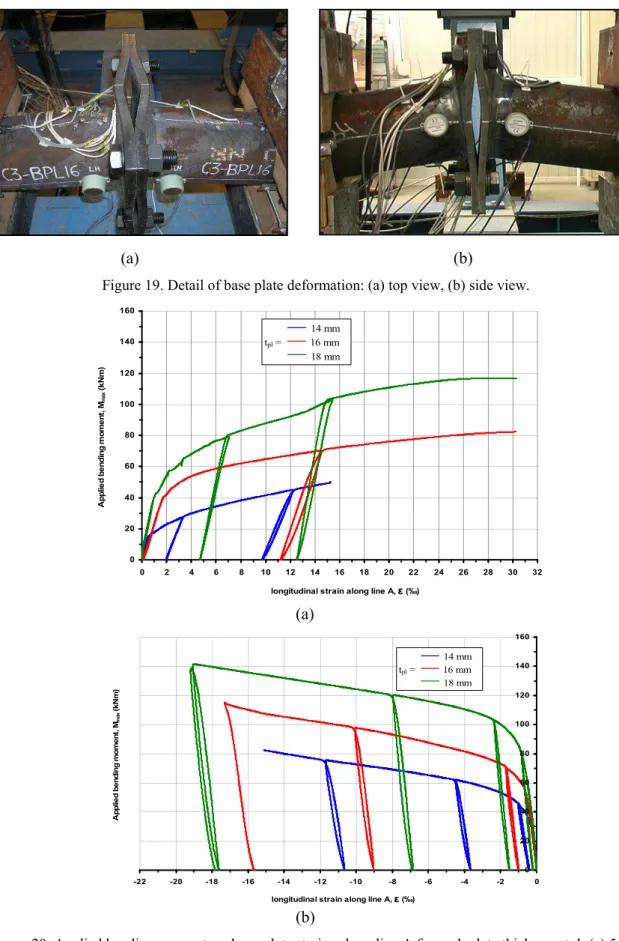
Under monotonic loading, the specimens with the larger base plate thickness showed higher flexural resistance at the same flexural deformation (or base rotation) and lower deformation at the same applied bending moment than those with the smaller thickness, as expected. The failure mode of the base plates are shown in Figure 19. The longitudinal strains along line A and C (Figure 16) changed sign from positive close to the weld-toe to negative towards the end of the plate (see Figure 20, Figure 21) causing reverse curvature in both sections A and C, with an inflection point at a distance of about 35 mm from the plate edge (more or less the line which connects the outside edge of the washers used for the bolts). On the other hand, tensile strains were measured in the transverse direction of line A (vertical section of plate) and C (horizontal section) with much larger values at the end of the plate than close to the weld-toe, causing 2 to 3 times higher transverse curvature along the vertical section than that in the horizontal section of the plate (axis of applied moment), as shown in Figure 19.
0 20 40 60 80 100 120 140 160 0 20 40 60 80 100 120 140 160 180 200 load-point deflection, δ (mm) M a x im u m b e n d in g m o m e n t, Μm a x ( k N m ) 14 mm 16 mm 18 mm 0 20 40 60 80 100 120 140 160 0 1 2 3 4 5 6 7 8 9 10 11 12
rotation at base, (degrees)
M a x im u m b e n d in g m o m e n t, Μ m a x ( k N m ) 14 mm 16 mm 18 mm
14 (a) (b)
Figure 19. Detail of base plate deformation: (a) top view, (b) side view.
(a)
(b)
Figure 20. Applied bending moment vs. base-plate strains along line A for each plate thickness, tpl: (a) 5 mm away from the weld-toe, (b) 80 mm away from the weld-toe.
0 20 40 60 80 100 120 140 160 0 2 4 6 8 10 12 14 16 18 20 22 24 26 28 30 32
longitudinal strain along line A, ε (‰)
A p p li e d b e n d in g m o m e n t, Μ m a x ( k N m ) 14 mm tpl = 16 mm 18 mm 0 20 40 60 80 100 120 140 160 -22 -20 -18 -16 -14 -12 -10 -8 -6 -4 -2 0 longitudinal strain along line A, ε (‰)
A p p li e d b e n d in g m o m e n t, Μ m a x ( k N m ) 14 mm tpl = 16 mm 18 mm
15
(a) (b)
Figure 21. Applied bending moment vs. base-plate strains along line C for each plate thickness, tpl : (a) 5 mm away from the weld-toe, (b) 80 mm away from the weld-toe.
0 20 40 60 80 100 120 140 160 0 2 4 6 8 10 12 14 16 18 20
longitudinal strain along line C, ε (‰)
A p p li e d b e n d in g m o m e n t, Μ m a x ( k N m ) 14 mm tpl = 16 mm 18 mm 0 20 40 60 80 100 120 140 160 -12 -10 -8 -6 -4 -2 0
longitudinal strain along line C, ε (‰)
A p p li e d b e n d in g m o m e n t, Μ m a x ( k N m ) 14 mm tpl = 16 mm 18 mm
16
II. Deliverable 3.2 : column specimens
CHS circular hollow section HSS high strength steel D diameter
t thickness
ID specimen identification S0 original cross sectional area D0 original cross sectional diameter L0 original gauge length
Rp0,2 stress at 0.2% of plastic extension Rm tensile strength
Ag percentage plastic extension at maximum force (percentage of the extensometer length) A permanent elongation after fracture expressed as a percentage of the original gauge length Z percentage reduction of area
εy the total strain (elastic + plastic) corresponding to Rp0.2 of the material σmax maximum stress of a stress controlled cyclic tests
σmin minimum stress of a stress controlled cyclic tests
ext res ,
σ
is the residual stress measured on the external surface;m
σ
is the membrane component of residual stress;b
σ
is the bending component of residual stress; E is the Young modulus of the material;l in the application of sectioning method is the strip length;
f in the application of sectioning method is the flexural deformation of a strip. ECCS European Convention for Constructional Steelwork
CFT concrete fillet tube
O ovality imperfections (Dmax-Dmin)/Dnominal e dimples or wrinkling imperfections
LVDT linear displacement transducer
Nmax in an axial load tests the maximum compressive axial load reached
du in an axial load tests the column shortening at maximum compressive axial Napply in a combined load test the applied compressive axial load
Mmax in a combined load test the maximum bending moment reached
17
II.1. Mechanical characterization of materials
Two (2) different CHS made of HSS nominal strength grade S590 from seamless quenched and tempered products were studied:
Cross-section A diameter (D) = 355 mm thickness (t) = 12 mm Cross-section B diameter (D) = 323.9mm thickness (t) = 10 mm Material testing programme performed is summarized in Table 2
Table 2. Material characterization testing program.
Test Nr. of test
Tensile test at room temperature 4
Cyclic test at room temperature 10
Hole drilling 8
Chemical composition 4
Microstructural analysis and hardness 8
Material thoughness 4
Sectioning method 2
II.2. Tensile tests
Two (2) tensile tests each cross-section were performed at room temperature in accordance with [7]. Specimens were cylindrical (7 mm in diameter) machined in longitudinal direction. Results are reported in Table 3 and Figure 22.
Table 3. Results of tensile test at room temperature.
Cross
ID S0 D0 L0 Rp0,2 Rm Ag A Z
section mm² mm mm MPa MPa % % %
A A-1 37.72 6.93 50 746 821 7.2 16 72
A-2 37.72 6.93 50 733 811 6.8 15 72
B B-1 38.16 6.97 50 723 805 7.3 16 72
18
Figure 22. Room temperature tensile tests on CHS: engineering stress vs. engineering strain.
II.2.1. Cyclic tests
Five (5) cyclic tests each cross-section were performed on cylindrical specimens (6 mm in diameter) machined in longitudinal direction. Testing programme and loading specifications are reported in Table 4 where
εy the total strain (elastic + plastic) corresponding to Rp0.2 of the material σmax maximum stress of a stress controlled cyclic tests
σmin minimum stress of a stress controlled cyclic tests
Table 4. Testing programme and loading conditions for material cyclic tests.
Cyclic test Strain/stress range
specimen ID
Cross section A Cross section B Strain controlled cyclic
tests
± 2 εy A-1 B-1
± 1.5 εy A-2 B-2
Stress controlled cyclic tests
σmax = σ (2 εy) ; σmin = 0 A-3 B-3
σmax = σ (2 εy) ; σmin = - 0.4
σmax A-4 B-4
σmax = σ (2 εy) ; σmin = - 0.8
σmax A-5 B-5
Each cyclic test was continued up to 100 cycle were completed, no premature failure was recorded. Whole test data are available up to 30th cycle, after the 30th cycle 1 each 5 cycle performed was recorded. Results are summarized in Table 4 and Table 5 for strain and stress controlled tests respectively. Stress softening (Table 5) and strain stabilization (Table 6) are evaluable.
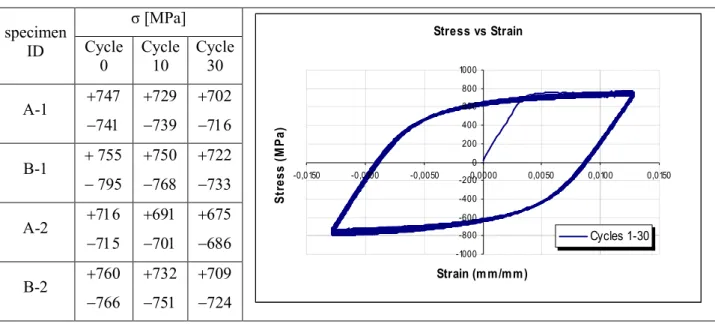
Table 5. Results of strain controlled cyclic tests. Strain controlled cyclic test B-1.
specimen ID σ [MPa] Stress vs Strain -1000 -800 -600 -400 -200 0 200 400 600 800 1000 -0,0150 -0,0100 -0,0050 0,0000 0,0050 0,0100 0,0150 Strain (m m/mm) S tr e s s ( M P a ) Cycles 1-30 Cycle 0 Cycle 10 Cycle 30 A-1 +747 −741 +729 −739 +702 −716 B-1 + 755 − 795 +750 −768 +722 −733 A-2 +716 −715 +691 −701 +675 −686 B-2 +760 −766 +732 −751 +709 −724
19
Table 6. Results of stress controlled cyclic tests. Stress controlled cyclic test B-4.
specimen ID ε x 10-2 Stress vs Strain -400 -200 0 200 400 600 800 1000 0,0000 0,0020 0,0040 0,0060 0,0080 0,0100 0,0120 0,0140 0,0160 Strain (m m/mm) S tr e s s ( M P a ) Cycles 0-30 Cycle 0 Cycle 10 Cycle 30 A-3 +1.08 +0.70 +1.15 +0.77 +1.19 +0.81 B-3 +1.31 +0.90 +1.37 +0.97 +1.40 +1.00 A-4 +1.08 +0.47 +1.20 +0.65 +1.28 +0.73 B-4 +0.31 +0.64 +1.41 +0.81 +1.46 +0.88 A-5 +1.05 +0.072 +1.38 +0.37 +1.87 +0.82 B-5 +1.46 +0.14 +2.01 +0.79 +3.32 +0.19
II.2.2. Residual stresses
Heat treated products as those under study are expected to show very low level of residual stresses (about 5-15% of yield stress).
As first attempt the hole drilling technique was applied to measure residual stresses. This technique is a semi-destructive one and measure via electrical strain gauges the evolution of residual strains relaxation while removing a little quantity of material by drilling. Four (4) measurements on each of the two (2) cross sections A and B were performed producing a total of 8 measuring points.
Since higher value than those expected have been measured (about 200MPa) extra investigations were planned. In particular:
• Material characterization to verify the effectiveness of tempering process (chemical composition, metallographic inspections, hardness and thoughness).
• Residual stress measurements applying another technique: the method of sectioning.
a. Material characterization
When substantial variation of residual stresses is expected it should be coupled with variation of metallurgical quantities as grain size and material hardness. Metallographic inspections and hardness HV10 measurements were performed in 4 different positions through each cross-section and 3 different depths each position. Moreover chemical composition and material toughness have performed. The data obtained shown no substantial variation of metallurgical quantities thorough thickness and in the different positions analyzed, that is in accordance with the heat treatment experienced by the material.
20 245 250 255 260 265 270 275 280
Outside Diam Mid Diam Inside Diam
h a rd n e s s H V 1 0 A B C
Figure 23. Hardness through thickness of three different CHSs. Table 7. Impact test Charpy V.
Cross section-ID Temp. [°C] Energy [J] Brittle area [%] A-1 - 20 172 15 A-2 - 20 175 20 B-1 - 20 162 20 B-2 - 20 178 15 C-1 - 20 148 0 C-2 - 20 147 0 OD
21 MD
ID
Figure 24. Microstructure analysis of CHS A (355 x 12 mm).
22 MD
ID
Figure 25. Microstructure analysis of CHS B (323.7 x 10 mm).
b. Sectioning method
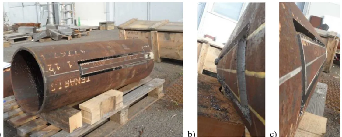
The “sectioning method” [8] was selected by the Consortium for a deeper evaluation of longitudinal residual stresses. This method consists of the extraction of a cross-section and its sectioning in several strips. It is based on the principle that internal stresses are relieved by cold-cutting the specimen. The stress distribution over a cross section can be determined with reasonable accuracy by measuring the change in length of each strip and by applying Hooke’s Law. Substantial variation through thickness of longitudinal residual stress is detected via measuring eventual deflection of strips after cutting. While historically the change in length of the strips was measured by means of mechanical extensometers recently the application of electrical strain gauges has proved its benefits [9]and the present application refers to the latter.
The sectioning method was applied on cross section A (Figure 26): a 2m long specimen was instrumented with electrical strain gauges on the external surface at mid span; allowing to the record of both longitudinal and transversal strains relaxation during sectioning. Test piece was extracted and subsequently sectioned by cold sawing (Figure 27) and data acquisition was continued during those operations.
23
Figure 26. Sectioning method: instrumented specimen before during and after sectioning.
Longitudinal residual stresses were measured on the external surface (
σ
res ,ext) and its distribution through cross section is reported in Figure 27. Longitudinal residual stresses are in the range of (-20 MPa ; + 63 MPa ) in accordance with the heat treatment experienced by the products.Figure 27. Sectioning method: cross section A after sectioning (left) and longitudinal residual stress distribution through cross section A (right) measured on the external surface.
Flexural displacements due to through thickness variation of residual stresses were evaluated by the application of the method of Anderson-Fahlman [10]. It consists on cold cutting a longitudinal strip of appropriate length (l) and measuring its flexural deformation (f), bending residual stress (
σ
b) being obtained by the formula:2
l Etf
b =
σ
andσ
res,ext =σ
b +σ
mwhere:
ext res ,
σ
is the residual stress measured on the external surface;m
σ
is the membrane component of residual stress;b
σ
is the bending component of residual stress; E is the Young modulus of the material; t is the CHS thickness;24 l is the strip length;
f is the flexural deformation.
In the present case two (2) strips 800mm long were milled (Figure 28). On one of the two milled strips 15 MPa of bending residual stress (+ 15MPa on the external surface and – 15MPa on the internal surface) were measured while on the other strip no relevant flexural deformation was detected.
a) b) c)
Figure 28. Application of the method of Anderson-Fahlman: a) specimen; b) deflected strip; c) not deflected strip.
II.2.3. Discussion and conclusions
Products under study are HSS seamless quenched and tempered tubes. Several different material tests have been performed and main results are listed below:
• Material strength is well above the S590 nominal strength class, in fact its actual resistance can be classified as S690 steel grade.
• Material cyclic tests were performed with the scope of defining material behaviour for finite element modelling (task 5.1): stress softening and strain cyclic stabilization were well detected with constant strain and constant stress cyclic tests respectively.
• Residual stresses were measured via the application of the method of sectioning: very low values of residual stress (about 10% of yield stress) were measured in accordance with the heat treatment experienced by these products.
II.3. Tests on column specimens
Eighteen (18) full scale monotonic tests were performed on HSS CHS columns made from seamless quenched and tempered products. Cross section dimensions and classification in accordance with EN 1993-1-1 and EN1993-1-12 are reported in the following table.
Table 8. Cross sectional dimensions of specimens.
ID diameter D [mm] thickness t [mm] D/t Nominal S590 Class Actual S690 Class A 355 12 29.6 3 3 B 323.9 10 32.4 3 4
As cross sectional classification depends also on yield strength of materials, both actual and nominal values of yield stress are considered in Table 8. In the following of this task only actual value of yield stress is considered.
The full scale testing arrangement is shown in Figure 29 where a Bs specimen is ready to be tested. Bending moment is applied at column ends leading to uniform bending along the column. Columns are connected to the machine hinges via two symmetric extensions (1.5 m long for long specimens and 2.0 m for short specimens), the second order moment generated by is taken into account in the elaboration of experimental data performed in Task 6.2.
25
Figure 29. Column Bs arranged in the testing machine before testing.
With the scope of reducing time needed for the testing arrangement, dedicated testing grips have been designed and fabricated. Hence full scale column specimens have been delivered with base column flanges to be bolted on the dedicated frame grips (Figure 30).
Each cross section was tested in two different column lengths:
• Short column (1850mm) relevant for cross sectional behaviour • Long column (4850 mm) relevant for member behaviour
Loading conditions applied are several different combinations of axial compressive load (N) and bending moment (M) as detailed in Table 9. In this way main points of M-N interaction diagrams can be checked.
Figure 30. Full-scale column test: one of the testing grips dedicated to column test of the project and column specimens delivered with stiffened flanges.
Table 9. Testing program for monotonic full scale tests
Cross section
Class EN
1993-1-12
Short column Long column
slenderness Nr. of tests slenderness Nr. of tests Pin ends Fixed ends Pin ends Fixed ends A 3 15 7.6 Nr. 5 tests: - 1 N - 4 N+M 40 20 Nr. 4 tests: - 1 N - 3 N+M B 4 17 8.3 Nr. 5 tests: - 1 N - 4 N+M 44 22 Nr. 4 tests: - 1 N - 3 N+M
26 II.3.1. Geometrical measurements before testing
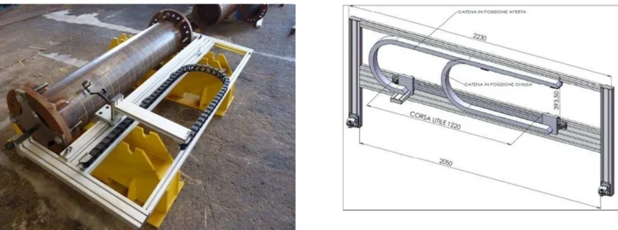
The actual dimensions of columns (thickness, diameters and outer profile) were measured before testing so as to characterize geometrical imperfections relevant for cross sectional and/or member stability. The geometrical survey of the outer profile was performed employing a measuring equipment, developed and realized for the scope. It is composed by an aluminium stiff reference frame able to rotate around a reference axis of the column and equipped with a sliding guide supporting an LVDT which is always in contact with the column outer profile (Figure 31). It allow to obtain actual diameters (D), ovality imperfections (O = (Dmax-Dmin)/Dnominal) and dimples (wrinkling) imperfections (e).
Figure 31. Actual geometry measurements: measuring device arranged on short specimen.
Thickness (t) distribution has been measured on the short column to be tested under combined loading. Three cross sections have been measured each column, using ultrasonic device for thickness for the diameters.
Maximum deviations of the above dimensions (D, O, t and e) from the nominal values are summarized in Figure 32 while complete set of measurements are available in the following sections.
A comparison with tolerances reported in the relevant standard of products [13] was also performed. It can be noted that columns actual dimensions are in accordance with and satisfy the admissible tolerances reported in Table 10.
Table 10. Dimension tolerances reported in EN 12010-2:2006 [7].
dimension ID tolerance
Diameter D ± 1 %
Thickness t
- 10 % (the positive deviation of thickness is implicitly limited by the tolerance on the mass: ± 6 % on each
delivered member length)
Ovality O 2 %
27
Figure 32. Measurement of geometrical imperfections: deviations from nominal dimensions of column specimens.
II.3.2. Axial compression tests
Four (4) tests were conducted in pure axial compression and fixed ends conditions. The load was applied at a constant displacement rate of 1.7mm/min.
Columns instrumentation is listed below:
• nr. 12 strain gauges on circumferential positions through 3 different cross sections; • nr. 4 LVDT in axial direction on circumferential positions ;
• specimens were grid marked with a 50mm edge square grid; • evolution of global deformation process by video-recording. The test results are summarized in Table 11.
Table 11. Axial compressive test results.
specimen ID slenderness Nmax [kN] du [mm]
nominal actual delta
Short column As1 7.6 9556 10254 + 7.30% 10.4 Bs1 8.3 6449 7961 + 23.4% 8.79 Long column Al1 20 9307 10857 + 16.7% 18.7 Bl1 22 6171 7812 + 26.6% 17.0
In the figures below the load-displacement curves obtained from short column tests and long column tests are reported together with photographs of the columns after testing.
28
Figure 33. Axial compression tests: load vs. shortening diagram
Figure 34. Axial compression tests: short column after testing As1 (left) and Bs1 (right).
Figure 35. Axial compression tests: long column Al1 after testing.
The geometry of bulge developed during the test was measured and is available in the following sections.
29 II.3.3. Combined axial and bending tests
Fourteen (14) full scale tests have been performed under combined loading condition and free end rotations. Testing procedure consists of axial load increase at a constant rate up to the desired value then while axial load is hold fixed, slowly increase of the bending moment.
The columns were instrumented as listed below:
• nr. 4 strain gauges on 4 circumferential positions at mid span cross section; • nr. 2 LVDT in axial direction (positions 90° and 180°);
• nr. 2 LVDT to measure column transversal displacement; • hinges rotation;
• evolution of global deformation process by video-recording.
Some photographs of the specimen after testing are reported in Figure 36. In Table 12 results obtained on short columns are summarized.
Figure 36. Column Bs3-13 and column As3- 13 after testing.
Table 12. Combined loading tests: short column results.
ID Napply [kN] Mmax [kN m] ΦΦΦΦu [degrees]
As3-13 1340 891 2.6 As3-25 2500 732 1.9 As3-50 5000 377 1.1 As3-75 7600 102 0.4 Bs3-13 1000 575 2.4 Bs3-25 1865 492 1.8 Bs3-50 3980 209 1.0 Bs3-75 5822 76 0.5
30
Figure 37. Combined loading tests: short column Moment vs. Rotation curves.
In Table 13 results obtained on long columns are summarized.
Table 13. Combined loading tests: long column results.
ID Napply [kN] Mmax [kN m] ΦΦΦΦu [degrees]
Al3-25 1530 670 4.4° Al3-50 2590 441 3.3° Al3-75 4588 150 1.7° Bl3-25 1000 450 4.2° Bl3-50 2020 232 3.0° Bl3-75 3298 79 1.5°
Complete moment vs rotation diagrams obtained for long columns are shown in Figure 38.
Figure 38. Combined loading tests: long column Moment vs. Rotation curves.
31
Figure 39. Columns (left to right) Al3-50 Bl3 – 25 Bl3-50 Bl3-75 after testing.
Measurements of ovalization after testing are available in the following sections Extensive discussion of experimental data obtained is reported in Task 6.2.
III. Deliverable 3.3 : Beam-to-column joint specimens
III.1. Beam-to-column joints
Figure 40 shows the full scale beam-to-column joint realized by the use of tubular members in HSS S590.In agreement with the results of the design of the prototype structures andcomplying with the capacity design rule, the joints were realized with:
• composite beams HE280B S275 + concrete slab 55mm • composite columns 355,6x12 HSS S590 grade;
• connection of the beams to the column realized by means of horizontal andvertical plates S355 welded to the column and bolted to the beams by the use of cover plates and of M20 and M27 bolts Class 10.9.
32
Figure 40. Realization of beam-to-column joints at the UNITN Laboratory
Together with the finalisation of the detailing of the joints, the test set-ups weredesigned too. With reference to the proposed joint solutions, a scheme of the experimental set-up is shown in the Figure 41. The full-scale specimens were fixed to the set-up equipment in three points:
• at the base of the column, a hinge and a system of 8 bolts fixed the column tothe set-up equipment. The bottom part of the column was much more rigid andtransferred the shear forces without significant deformation.
• at the top of the column was fixed to the actuator with a system of 8 bolts. It should be well fixed so that the force and displacement of the actuator would be fully transferred to the joint. • at the far end of the beam was connected to a pendulum with a system of 8 bolts.With this type
of set-up, it allowed no transformation of the moment andhorizontal force from this end of the beam to the ground and no verticaldeformation of the beam.
33 The loads were applied by the actuator that was fixed horizontally to the reaction wall of the laboratory. Displacement control was used in order to simulate the actual earthquake situations. In both cyclic and monotonic test, the actuator was connected by the hinge system on top of the column to transfer the force and displacement.
The following instrumentswere used during testing:
•
Seika inclinometers that surveyed the distortion of the joint and the rotationsbetween beam and column;Figure 42. Inclinometers position
• LVDT transducers that surveyed the displacement between column and slab, beam and slab and the distortion of the joint;
34
Figure 44. LVDTs position on the beam and on the joint
• Strain gauges that survey the deformation both of the steel elements of thecomposite beams in the zone of the plastic hinges and of the re-bars into theslab to monitor the activation of the compression transfermechanism from the concrete slab into the column.
35
Figure 46. Strain Gauges position on re-bars
Figure 47. Strain Gauges position on flanges’ beam
36
III.2. Beam-to-column through-plate component
This experimental task includes four (4) to-column tests to study the response of four (4) beam-to-column through-plate specimens (denoted as Component 2) under compression. The CHS 323.9x10 steel tubes (produced by Tenaris Dalmine) are made of high-strength steel (TS590- fy=735 MPa) and
the HEM280 beams and through-plates of S355 steel. The parts of the specimens were manufactured by Stahlbau Pichler.
III.2.1. Test Instrumentation
For the Component 2 tests, four (4) geometries of steel through-plates were studied, as shown in Table 1. For the Component 2 tests, 3-point bending was applied to the simply supported specimens through an actuator bolted to the top of the column tube as shown in Figure 49. The instrumentation setup for this type of test consisted of wire position transducers to measure load-point displacements, DCDT’s for measuring support displacements and a number of axial and biaxial strain gages which were attached to the through-plates (see Figure 50a) and column tube (see Figure 50b).The specimens were subjected to monotonic 3-point bending (stroke rate=0.1 mm/sec).
Figure 49. Test setup for Component 2 specimens
(a) (b)
37 III.2.2. Experimental Results
As far as the ultimate bending capacity is concerned, the specimen with the 120x10-mm steel plate resisted a bending moment of 189.7 kNm, that with 120x12-mm plate a bending moment of 185.4 kNm and the specimen with a 100x12-mm plate a bending moment of 191.2 kNm (see Table 14). There is a kink in all load-deflection curves shown in Figure 3 due to slipping of the bolted connections along the span of the beam, so the true estimated load-point displacement at failure is about 10÷12 mm.
The general view of a deformed specimen is shown in Figure 52. More specifically, the specimen with the 100x15-mm through-plate failed due to lateral buckling of the plate outside the column tube at a bending moment of 221.2 kNm (Figure 53), while the specimens with the 120x10-, 120x12- and 100x12-mm through-plates under monotonic loading failed due to buckling of the through-plate inside the column tube (see Figure 54). The flexural capacity of the three (3) specimens was, at load point deflections values, close enough. It seems that for the considered differences in plate height and thickness, the flexural response is very similar. Conversely, the specimen with the thickest and shortest 100x15-mm through-plate, which failed due to lateral buckling of the plate outside the column tube (see Figure 53b), exhibited about 17% higher flexural capacity than the other three specimens.
Table 14. Experimental results for Component 2 tests.
specimen type height of through-plate, thickness of through- plate, tpl ( mm)
bending moment at plate failure, Mmax (kNm) Component 2 120 10 189.7 120 12 185.4 100 12 191.2 100 15 221.2 0 50 100 150 200 250 300 0 5 10 15 20 25 30 35 40 load-point deflection, δ (mm) M a x im u m b e n d in g m o m e n t, Μ m a x ( k N m ) plate 100x12 plate 100x15 plate 120x10 plate 120x12
Figure 51. Applied bending moment vs. LP displacement diagram for Component 2 specimens under monotonic loading.
38
Figure 52. Deformed Component 2 specimen
(a) (b)
Figure 53. Failure of the through-plate for specimen (100x15): (a) buckling inside the column tube, (b) lateral buckling outside the tube.
Figure 54. Failure of the through-plate for the remaining three (3) specimens. Buckling of through-plate inside the tube
39
III.3. Slab reinforcement component
This experimental investigation consists of four (4) tests on composite slab (denoted as Component 1) to determine the flexural response of the concrete slabs used in the structural joints tested at the University of Liege (two specimens) and the University of Trento (two specimens). Three (3) of the composite slab specimens under consideration (1.1, 1.2, and 1.3a) have been subjected to monotonic bending loading, whereas the forth specimen (1.3b) to cyclic bending loading (ECCS loading protocol) with the slab in tension.
Each of the specimens consists of a concrete slab, resting on a thin steel sheeting and supported by a heavy steel beam of section HEM 280 from S355 material, as shown in Figure 55. Each specimen also contains a steel tube, made of high-strength steel (TS590), with a nominal yield stress of 735 MPa, located in the middle of the slab, simulating the steel column. The two specimens similar to the ones tested in Liege, are denoted as specimens 1.1 and 1.2 and have the following characteristics:
• Steel beams: HEM 280 (S355) • Steel tube 323.9 × 10 mm (TS590)
• Concrete slab: thickness h=16 cm, nominal compressive strength C30/37 • Sheeting: Cofraplus 60 (S275), t =0.75 mm
• Longitudinal steel rebars 10Ø10 and 6Ø10 (B450-C) • Transverse steel rebars Ø10/100 (B450-C)
• Studs 19×125/100
The two specimens similar to the ones tested in Trento, are denoted as specimens 1.3a and 1.3b, and have the following characteristics:
• Steel beams: HEM 280 (S355) • Steel tube: 355.6 × 12.5 mm (TS590)
• Concrete slab: thickness h=12 cm, nominal compressive strength C30/37 • Sheeting : Fe250 G (fy=250 MPa), t=1.0 mm
• Longitudinal steel rebars 10Ø10 and 6Ø12 (B450-C) • Transverse steel rebars Ø10/100 (B450-C)
• Studs 19×125/100
Specimen 1.3a has been subjected to monotonic flexural loading and specimen 1.3b to cyclic flexural loading, with the slab in tension.
40
Figure 55: General views of concrete slab specimens.
The steel reinforcement arrangement of the concrete slabs is shown in Figure 56. Before casting of the concrete slabs, appropriate instrumentation (with strain gages) was done in specific rebars, as shown in Figure 56c and Figure 56d. A detailed configuration of instrumentation for specimens 1.1 and 1.3 is shown in Figure 57 and Figure 58, respectively. The 28-day cube compressive strength of the concrete used is 40.4 MPa.
(a) (b)
41
(e) (f)
Figure 56: Preparation of concrete slab specimens: (a) specimen 1.1; (b) specimen 1.2; (c) instrumentation of specimen 1.1 ; (d) instrumentation of specimen 1.2; (e) specimen 1.3; (f) instrumentation of specimen 1.3.
3 10 3 10 323,9 3224 1 0 0 0 200 200 310 310 s1.1 s2 s3 s1 s2 s3 m1.1 m1.2 m1.3 s1.3 s1.2
Figure 57. Instrumentation of concrete slab specimen 1.1.
1 0 0 0 3456 355,6 mesh 10/100x100 3 12 3 12 s1 s2 s3 s1.1 s2 s3 s1.2 s1.3 m1.1 m1.2 200 200 310 1 2 0 8 0 8 0
42 The experimental 4-point bending loading set-up is shown schematically in Figure 59. The specimens are supported at two points in the middle region, whereas vertical loading is applied through a cross-beam at the two ends of the specimens, so that a constant negative bending moment (slab in tension) is developed and the middle section of the slabs.
HEM 280
a
a
b
c
b
δ
δ
(a) HEA300 2770 22 75 IPE 360 FLOOR 40 23 55 HEA240 40 25 concrete slab steel sheeting steel beam hydraulic jack (b)43
(c) (d) (e)
Figure 59: Loading set-up for the composite concrete slab specimens.
type of
specimen specimen loading type of
flexural capacity (kNm) Reinforced concrete slabs (component type 1) 1.1 monotonic
329.7
1.2 monotonic331.8
1.3a monotonic264.0
1.3b cyclic290.0
The experimental results are summarized in the above Table, and the failure modes of the composite specimens 1.1, 1.2, 1.3a and 1.3b are shown in Figure 60, Figure 61, Figure 62 and Figure 63, respectively.
(a) (b)
Figure 60: Flexural behavior of composite slab specimen 1.1 under monotonic loading: (a) detail of cracking development, (b) debonding of steel sheeting and excessive flexural deformation of the slab.
44
(a) (b)
(c) (d)
Figure 61: Flexural behavior of composite slab specimen 1.2 under monotonic loading: (a) initiation of concrete cracking, (b) development of further cracking, (c) debonding of steel sheeting, (d) final stage: excessive concrete cracking.
(a) (b)
Figure 62: Flexural behavior of composite slab specimen 1.3a under monotonic loading: (a) detail of cracking development, (b) debonding of steel sheeting and final stage: excessive flexural deformation.
45 (a)
(b) (c)
Figure 63: Cyclic flexural response of composite slab specimen 1.3b: (a) detail of cracking development, (b) detail of excessive cracking around the tube and (c) general view of the final flexural deflection.
Several observations could be derived from the tests on the composite slab specimens. At first, the failure modes of specimens 1.1 and 1.2 are different from the ones of specimens 1.3. In the case of specimens 1.1 and 1.2, the cracks started from the tube perimeter and propagated along the tube’s radial direction (Figure 60). On a later stage the cracks opened progressively through the slab thickness. It was observed that for both specimens 1.1 and 1.2 the major cracks were mostly developed and propagated from the region around the tube circumference up to the stud closest to the tube. The cracks developed normal to the plane of bending near the studs closer to the tube, at both sides. On the other hand, in the case of specimens 1.3, the cracks started and propagated along a circular perimeter around the tube (Figure 62 and Figure 63) at a distance equal to the length of the studs placed radially around the tube wall. In particular, specimen 1.3b exhibited a very ductile behaviour. Both specimens 1.3a and 1.3b showed more distributed cracking throughout the concrete slab, while specimens 1.1 and 1.2 showed more localized cracking in the middle region of the slab and higher flexural capacity. The structural behaviour of the slab components is identified by the moment-displacement curves traced during the monotonic and cyclic tests (Figure 64, Figure 65).
46 0 50 100 150 200 250 300 350 400 0 10 20 30 40 50 60 70 80 90 100 110 120 load-point deflection, δ (mm) A p p li e d b e n d in g m o m e n t, Μ ( k N m ) specimen 1.1 specimen 1.2
Figure 64. Moment – deflection curves for specimens 1.1 and 1.2.
0 50 100 150 200 250 300 350 400 0 10 20 30 40 50 60 70 80 90 100 110 120 load-point deflection, δ (mm) A p p li e d b e n d in g m o m e n t, Μ ( k N m ) specimen 1.3a specimen 1.3b δy/4 δy 3δy/4 δy/2 3δy 2,5δy 2δy 4δy 3,5δy
Figure 65. Moment – deflection curves for specimens 1.3a and 1.3b.
III.4. Experimental results on joints
III.4.1. Types of test
Cyclic and monotonic tests were performed on beam-to-column joints and column-base joints. In detail, the following tests were realized: i) monotonic tests; ii) cyclic tests according to the ECCS procedure (ECCS, 1986); iii) random tests. The aim of tests was to understand the global behaviour of joints and the activation of mechanisms in critical parts. Figure 66 shows the loading protocol applied to beam-to-column joints; the inputs of tests for beam-to-column-base joints are similar and not shown for brevity.
47 a. Monotonic test
The monotonic test was realized in order to estimate the maximum force level and the maximum rotational capacity of the joint and the position of plastic hinges. Figure 66 shows the loading protocol applied; test was carried out in displacement control, on beam-to-column joint with maximum displacement imposed of about ±240mm.
Figure 66. Loading protocols relevant to tested beam-to-column joints
b. Cyclic test
Cyclic tests were performed in order to evaluate the hysteretic behaviour of joints, the degradation of strength and stiffness with the increasing of damage level as well asthe rotational capacity under cyclic loadings. The cyclic test was realized according to the ECCS stepwise increasing amplitude loading protocol (ECCS, 1986), modified with the SACprocedure (Karl et al., 1997). The stepwise was evaluated considering an interstorey drift angle equal to 5 mrad, in order to evaluate the benchmark displacement ey= 0.005h, where h is the storey height equal to 3.5 m. The loading protocol was divided
into the two following parts: • one cycle in the intervals:
/ 4,
/ 4; 2,
/ 4, 2
/ 4;3
/ 4,3
/ 4;
,
y y y y y y y y
e
+e
−e
+e
−e
+e
−e e
+ −• three cycles in the intervals:
2 , 2 ; 4 , 4 ;...;(2 2 ) , (2 2 )
e
y+e
y−e
+ye
y−+
n e
y++
n e
y−withn=1,2,3,...The maximum displacement reached in the test on beam-to-column joint was 12ey equal about to ±
210mm, corresponding to the available stroke of the actuator. Conversely, in the case of column-base joints it was possible to reach a displacement of ±16eyequal to about ±140mm, due to height of
specimens, which is equal to half height of the beam-to-column specimen. c. Random test
The aim of random tests was the characterizationof the actual behaviour andperformance of joints under seismic loading.The random testswere performed using as input the interstorey drift provided by the non-linearstructural analysis of the 2D frame developed in WP2. The 2D frame was subjected to seismicloading by means of a far field spectrum-compatible accelerogram, in agreement with theEN1998-1 (2005). The value of the peak ground acceleration was increased about to 1,8g, to obtain the displacements in loading protocol comparable to that maximumrecorded during the ECCS test. The response of the 2D frame was scaled in time to obtain quasi-static cyclic tests.
Figure 67 shows the 2D frame used to evaluate the loading protocol of the random test by non-linear analysis, considering two plastic hinges in parallel located at beam ends. In detail, the displacement at the middle height of the first story column depicts the input for tests on column-base joints.
48
Figure 67.Moment resisting frame model used to evaluate loading protocol for the random test
III.4.2. Column-base joints
Figure 68 shows the test set-up ofcolumn-base jointstested under cyclic loading protocols, according with the ECCS procedure and with random loadings up to collapse.
Figure 68.Axonometric view of Column-base joint
Table 15 shows the 6 tests realized on column-base specimens.
Table 15. Specimen nomenclature and test protocol
Number Label Test Protocol Type of Specimen
1 CBJSTE ECCS-SAC Column-base joint designed for static loads 2 CBJSTR RANDOM Column-base joint designed for static loads 3 CBJSEE ECCS-SAC Column-base joint designed for seismic loads 4 CBJSER RANDOM Column-base joint designed for seismic loads 5 CBJINE ECCS-SAC Column-base joint with an improved s. design 6 CBJINR RANDOM Column-base joint with an improved s. design
a. Column-base joint designed for static loading
The collapse of the joint was associated with plastic deformation of the thin base plate, as shown in Figure 69.
displacement h/2
49
Figure 69.Column-base joint for static loads: Geometry and Failure;
Relevant hysteretic behaviour was characterized by high values of rotation without significant strength degradation, as showed in the following figures. The maximum force reached was equal to about 170 kN associated with a displacement of about 175 mm.
-1000 -500 0 500 1000 -15 -10 -5 0 5 10 15 Displacements [%] Force [kN] -1200 -800 -400 0 400 800 1200 -120 -80 -40 0 40 80 120 Rotations [mrad] Moment [k Nm]
Figure 70.CBJSTEcolumn-base joint; Force-interstorey drift curves and Moment-rotation relationships
-1000 -500 0 500 1000 -15 -10 -5 0 5 10 15 Displacements [%] F o r c e [ k N ] -1200 -800 -400 0 400 800 1200 -120 -80 -40 0 40 80 120 Rotations [mrad] M o m e n t [ k N m ]
Figure 71.CBJSTRcolumn-base joint; Force-interstorey drift curves and Moment-rotation relationships
b. Standard column-base joint designed for seismic loads
The stiffeners welded on the thick base plate permitted to obtain enough strength of the joint, see Figure 72. The ductile behaviour exhibited from the standard joint was correlated to the development of the plastic hinge at the base of the column. The collapse of the joint was due to failure of anchor bolts for high value of the plastic rotation of about 45 mrad. Until failure, the stiffness and strength degradation was negligible. The behaviour recorded during the test is showed in Figure 73 and in Figure 74, respectively.
50 -1000 -500 0 500 1000 -15 -10 -5 0 5 10 15 Displacements [%] F o r c e [ k N ] -1200 -800 -400 0 400 800 1200 -120 -80 -40 0 40 80 120 Rotations [mrad] M o m e n t [ k N m ]
Figure 73.CBJSEEcolumn-base joint; Force-interstorey drift curves and Moment-rotation relationships
-1000 -500 0 500 1000 -15 -10 -5 0 5 10 15 Displacements [%] F o r c e [ k N ] -1600 -1200 -800 -400 0 400 800 1200 1600 -120 -80 -40 0 40 80 120 Rotations [mrad] M o m e n t [ k N m ]
Figure 74.CBJSERcolumn-base joint; Force-interstorey drift curves and Moment-rotation relationships
c. Innovative column-base joint designed for seismic loads
The aims of tests on the innovative seismic base joint, realized by means of a column embedded in the foundation, were two: i) the evaluation of the hysteretic behaviour of joint under seismic actions; ii) the study of the mechanism of transfer of force between the column and the foundation, similar to the Strut & Tie mechanism proposed in EN 1992-1-1 (2005). The base joint exhibited stiffness and strength higher than the ones provided by the standard solution. This joint showed ductile behaviour characterized by large plastic rotation of about 45 mrad with brittle failure on weld between the column and the base plate, due to phenomena of local instability in the wall of the column. The hysteretic behaviour exhibited two plastic hinges on the column: i) one plastic hinge was located in the plinth due to compression of the concrete filling consequent to the rotation of the column; ii) a second plastic hinge located on the column outside of the plinth. To study the internal mechanism in plinths due to interaction between the column and the foundation strain gauges on the rebars in the plinths were welded. The tension recorded during the test permitted to check the validity of the numerical model set by the Abaqus program, to study the mechanical behaviour in the plinth
Figure 75.Innovative column-base joint for seismic loads: Geometry and Failure
-1000 -800 -600 -400 -200 0 200 400 600 800 1000 -15 -10 -5 0 5 10 15 Displacements [%] F o r c e [ k N ] -1200 -800 -400 0 400 800 1200 -120 -80 -40 0 40 80 120 Rotations [mrad] M o m e n t [ k N m ]
51 -1000 -500 0 500 1000 -15 -10 -5 0 5 10 15 Displacements [%] F o r c e [ k N ] -1200 -800 -400 0 400 800 1200 -120 -80 -40 0 40 80 120 Rotations [mrad] M o m e n t [ k N m ]
Figure 77.CBJINRcolumn-base joint; Force-interstorey drift curves and Moment-rotation relationships
d. Classification of column-base joints
With reference to column-base joints there is not a classification of the stiffness of the joint. In fact, column base joints subject to seismic action have to be designed to full rigid and full strength. In other European projects, it was observed that both the strength and stiffness of the standard solution depends of the behaviour of grout and anchor bolts. It is difficult to obtain a rigid and full strength joint. In order to show this, it was possible to compare the actual resisting moment of the CFT column with the moment recorder during the test in the plastic hinge. We obtained that: i) the standard solution is not over strength with respect to the column owing to grout cracking and anchor bolt elongation; ii) the innovative solution it is overstrength with respect to the column, in agreement with design. Figure 78
shows the comparison between aforementioned moments.
-1500 -1200 -900 -600 -300 0 300 600 900 1200 1500 -120 -80 -40 0 40 80 120 M o m e n t [ k N m ] Rotations [mrad]
SEISMIC JOINT
MRd,col= 1206 kNm -1500 -1200 -900 -600 -300 0 300 600 900 1200 1500 -120 -80 -40 0 40 80 120 M o m e n t [ k N m ] Rotations [mrad]INNOVATIVE JOINT
MRd,col= 1206 kNmFigure 78. Moment-Rotation of Seismic and Innovative Column-base joints
III.4.3. Beam-to-column joint
Figure 79 shows the test set-up of beam-to-column joints tested under loading protocols show in Figure 66.Table 16 summarizes the tests realized on beam-to-column joints.
Table 16. Specimen nomenclature and test protocol
Number Label Test Protocol Type of Specimen
1 BTCJE ECCS-SAC Beam-to-column Joint
2 BTCJR RANDOM Beam-to-column Joint
52
Figure 79.3D view of beam-to-column joints
Tested beam-to-column joints showed a ductile behaviour characterized by large rotations and values of strength without significant degradation. The only evident damage was spalling of concrete in compression near the column for high value of displacements. Plastic hinges were developed in the weaker sections between the plates weldedto the column and the beam ends. The formation of plastic hinges was associated with slip,for high value of displacement, both between the butt strap plates and the plates welded at the column and between the butt straps plates and the beam. The slip was due to clearances in the holes.
On the basis of mechanical and economic considerations, beam-to-column joints were realized without the connectors on the upper cover plate. Respect to similar joints tested in the past, these joints exhibit very limited stiffness and strength degradation to hogging moment. This is due to absence of instability phenomena in the bottom flange of beams. The relationship Force-Displacement on the top of the column and Moment-Rotation of plastic hinges recorded during testing are showed in following figures.
Figure 80.BTCJMbeam -to-column joint; Force-interstorey drift curvesand Moment-rotation relationships