HAL Id: hal-01761901
https://hal.archives-ouvertes.fr/hal-01761901
Submitted on 9 Apr 2020
HAL is a multi-disciplinary open access
archive for the deposit and dissemination of
sci-entific research documents, whether they are
pub-lished or not. The documents may come from
teaching and research institutions in France or
abroad, or from public or private research centers.
L’archive ouverte pluridisciplinaire HAL, est
destinée au dépôt et à la diffusion de documents
scientifiques de niveau recherche, publiés ou non,
émanant des établissements d’enseignement et de
recherche français ou étrangers, des laboratoires
publics ou privés.
Using Probabilistic Relational Models to Generate
Synthetic Spatial or Non-spatial Databases
Rajani Chulyadyo, Philippe Leray
To cite this version:
Rajani Chulyadyo, Philippe Leray. Using Probabilistic Relational Models to Generate Synthetic
Spatial or Non-spatial Databases. Research Challenges in Information Science (RCIS) 2018, 12th
International Conference on, May 2018, Nantes, France. pp.1-12, �10.1109/RCIS.2018.8406645�.
�hal-01761901�
Using Probabilistic Relational Models to Generate
Synthetic Spatial or Non-spatial Databases
Rajani Chulyadyo
1,2 1Capacit´es SAS University of Nantes Nantes, France [email protected]Philippe Leray
22DUKe research group, LS2N Laboratory UMR 6004
University of Nantes Nantes, France [email protected]
Abstract—When real datasets are difficult to obtain for tasks such as system analysis, or algorithm evaluation, synthetic datasets are commonly used. Techniques for generating such datasets often generate random data for single-table datasets. Such datasets are often inapplicable when it comes to evaluat-ing data minevaluat-ing or machine learnevaluat-ing algorithms dealevaluat-ing with relational data. To address this, our earlier works have dealt with the task of generating relational datasets from Probabilistic Relational Models (PRMs), a framework for dealing with prob-abilistic uncertainties in relational domains. In this article, we extend this work by proposing to use more efficient data sampling algorithms, and by using a spatial extension of PRMs to generate synthetic spatial datasets. We also present our experimental analysis on three different data sampling algorithms applicable in our method, and the quality of the datasets generated by them. Index Terms—probabilistic relational models, spatial data, synthetic data generation, relational data, bayesian networks, sampling
I. INTRODUCTION
Synthetic or artificial datasets are essential for evaluating data mining algorithms, database applications, or any system that deals with data and/or databases when it is expensive to evaluate them on real datasets. Many synthetic database generation tools can be found online. Tools such as DataFiller [1], ObjectFiller.NET [2], Generate Data [3], Faker [4], etc., populate databases with random data. However, evaluating data mining algorithms requires that the evaluation data have certain regularities. The data mining community has been concerned about the generation of such artificial data since a long time. A number of research works deal with artificial data generation for specific domains such as credit scoring [5], genetic study [6], intrusion detection [7], weather analysis [8] etc. [9] provides general methods for generating datasets for data mining algorithms. Synthetic data are also commonly used in the field of spatial data analysis. [10] provides a review of techniques for generating spatial microdata. Most works on synthetic data generation are built around the generation of single-table data, which is not suitable for evaluating algorithms that deal with the context where instances may be related to one another. Such relational context is very common in real world applications.
Existing tools that generate multi-table data often generate random data. However, to get synthetic relational data that
resemble real world data, we should consider dependencies among attributes or those among objects. One approach to achieve this could be to generate data probabilistically using a generative model, which typically uses probabilistic models to describe how data is generated. Among such generative models is a Bayesian network (BN) [11], which represents probabilistic dependencies among random variables as a graph. However, BNs can only model single-table (non-relational) data. Because BNs are among simple probabilistic graphical models (PGM) with intuitive graphical representation, and several algorithms for sampling a BN to generate unseen data are already available in the literature, we consider Prob-abilistic Relational Models (PRMs) [12], [13], an extension of Bayesian networks for relational settings, to generate syn-thetic relational data. In our earlier works [14], [15], we had proposed a method for generating (non-spatial) datasets using PRMs. In this article, we extend it to generate spatial datasets using PRMs with Spatial Attributes (PRMs-SA) [16], an extension of PRMs that support spatial objects. We will also discuss on three different data sampling techniques applicable in our framework, and present experimental results on the performance of the data generation algorithms, and the quality of generated datasets. Our dataset generation method serves as a method for benchmark generation not only for evaluating PRM learning and other relational learning algorithms but also for testing database applications.
This article is organized as follows. After a brief overview of the underlying techniques in Section II, we present our approach of generating spatial, and non-spatial datasets using PRMs in Section III. Experimental results on our approach of synthetic data generation are presented in Section IV. Conclusions are presented in Section V.
II. TECHNICAL BACKGROUND
A. Bayesian network (BN)
A Bayesian network (BN) [11] is a Directed Acyclic Graph (DAG) where nodes correspond to random variables and arcs between nodes represent conditional dependencies; lack of an arc between nodes indicates that the variables are conditionally
independent. A BN associates with each random variable Xia
conditional probability P (Xi| P ai), where P ai∈ X is the set
BN is conditionally independent of its non-descendants given its parent. This conditional independence assumption enables BNs to simplify the joint probability distribution given by the Chain rule as follows:
P (X1, X2, . . . Xn) =Y
i
P (Xi| P ai) (1)
We can make queries on BNs to infer about variables of interest. Several algorithms can be found in the literature for making inference on BNs.
B. Probabilistic Relational Model (PRM)
BNs have been one of the main models for reasoning under uncertainty. The simplicity of their specification is one of the reasons for their success. However, one of the difficulties in Bayesian networks is to create and maintain the model of very large domains, which are usually conceived with relational settings. BNs are not sufficient to model this construct as they lack the concept of objects and their relations. They are designed for modeling attribute-based domains, where we have a single table of independent and identically distributed instances [17], whereas real world data are often stored and managed using relational representation. Converting relational data into flat data representation for statistical learning may introduce statistical skew and lose useful information that might help us understand the data. Thus, in order to learn a statistical model from relational data, Probabilistic Relational
Models (PRMs)were emerged. A PRM specifies a probability
model for classes of objects rather than simple attributes. The structure of relational dataset is often described by a relational schema. Conversely, a dataset is an instance of a relational schema. A PRM defines a probabilistic model for a relational schema of the domain. Instantiating a PRM for a dataset results in a Bayesian network, also known as a Ground Bayesian Network (GBN), on which inference can be performed. In the following, we give formal definitions of these concepts.
A relational schema, denoted R, describes the classes, X , and the attributes, A, in a domain, and specifies the constraints over the number of objects involved in a relationship. Each class X ∈ X is described by a set of descriptive attributes A(X) and a set of reference slots R(X). A reference slot X.ρ relates an object of class X to an object of class Y and has Domain[ρ] = X and Range[ρ] = Y . The inverse of a
reference slot ρ is called inverse slot and is denoted by ρ−1.
While a reference slot gives a direct reference of an object with another, objects of one class can be related to objects of another class indirectly through other objects. Such relations are represented with the help of a slot chain, a sequence of
slots (reference slots and inverse slots) ρ1, ρ2, . . . ρn such that
for all i, Range[ρi] = Domain[ρi+1]. A slot chain can be single-valued or multi-valued. When it is multi-valued, we need a function such as mode, average, cardinality etc., to summarize them. We call such function an aggregator.
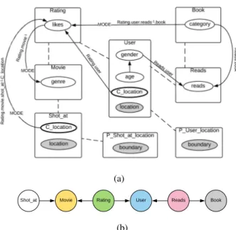
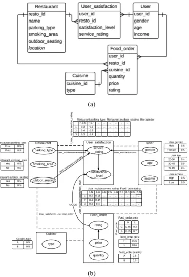
Fig. 1a depicts an example of a relational schema with 5
classes, X = { Restaurant,User satisfaction,Cuisine,Food order,
User}. Attributes other than identifiers form the set A.
Here, A(User satisfaction) ={satisfaction level, service rating}.
A descriptive attribute is also denoted as Class.attribute, e.g.,
User.age, Cuisine.type etc. Class User satisfaction contains two
reference slots, R(User satisfaction) = {user id, resto id}. The
former one, User satisfaction.user id, refers to the associated
Userobject, whereas the inverse slotUser satisfaction.user id−1
starts from theUserobject, and gives allUser satisfactionobjects
associated to theUserobject.User satisfaction.user id−1.resto id
is an example of a slot chain that gives all the restaurants that
have been rated by (i.e., related with) the givenUserobject.
Definition 1: Probabilistic Relational Model (PRM)
A PRM Π = (S, Θ) for a relational schema R is composed of a dependency structure S, and a set of parameters Θ [18]. The dependency structure S consists of a set of random variables and a set of probabilistic dependencies among the random variables. Each random variable X.A in S is a descriptive attribute A ∈ A(X) of a class X ∈ X , and has a set of parents Pa(X.A) = {U1, . . . Ul}, which describes probabilistic
dependencies. Each Uihas the form X.B or γ(X.τ.B), where
B is an attribute of any class, τ is a slot chain and γ is an aggregator of X.τ.B. Finally, the parameters Θ is a set of conditional probability distributions (CPDs), representing
P (X.A | P a(X.A)).z
Fig. 1b shows a PRM that corresponds to the relational schema in Fig. 1a. The dashed lines here indicate that the classes are linked through reference slots.
A dataset is an instance of a relational schema. An instance I of a schema can be complete (i.e., no missing values) or incomplete (i.e., missing or uncertain attributes, reference slots etc.). A special kind of partial instantiation of a relational
schema, where the set of objects σr(Xi) for each class and the
relations that hold between the objects are specified without specifying the values of the attributes, is called a relational
skeletonσrof the relational schema.
An example of a relational skeleton shown in Fig. 2a is an instance of the relational schema of Fig. 1a. Such skeleton describes how objects are related with each other in the dataset without specifying the attribute values.
Instantiating a PRM for a dataset results in a Bayesian net-work, also known as a Ground Bayesian Network (GBN). The process of generating a GBN involves copying the associated PRM for every object in skeleton σr. Thus, a GBN will have a
node for every attribute of every object in σrand probabilistic
dependencies and CPDs as defined in the PRM.
Definition 2: Ground Bayesian Network (GBN)
A ground Bayesian network (GBN) defined for a PRM Π and
a relational skeleton σr is as follows [13]:
• There is a node x.A for every attribute of every object
x ∈ σr(X).
• Each x.A depends probabilistically on parents of the
form x.B or x.K.B. If K is not single-valued, then the parent is the aggregate computed from the set of random variables {y | y ∈ x.K}, γ(x.K.B).
(a)
(b)
Fig. 1: An example of (a) a relational schema, and (b) a PRM
The joint distribution over the instantiations of a PRM, Π,
for a relational skeleton, σr is very similar to the chain rule
for standard Bayesian networks.
P (I | σr, Π) = Y X∈X Y A∈A(X) Y x∈σr(X) P (x.A | P a(x.A)) (2) Here, we need to ensure that the probability distributions are coherent, i.e. the sum of probability of all instances is 1. In Bayesian networks, this requirement is satisfied if the dependency graph is acyclic [13].
An example of a GBN (structure only), which is obtained by instantiating the PRM of Fig. 1b over the relational skeleton of Fig. 2a is shown in Fig. 2b. CPDs are not shown here due to space constraints. Colors are used only to distinguish the class of objects, and do not carry any significant meaning.
1) Inference in PRMs: The traditional approach to
inference in PRMs is to apply BN inference algorithms on the GBN obtained by unrolling a PRM for the given relational skeleton σr. Theoretically, standard inference
(a)
(b)
Fig. 2: An example of (a) a relational skeleton, and (b) a Ground Bayesian Network (GBN) obtained by unrolling the PRM of Fig. 1b over the relational skeleton.
algorithms for Bayesian networks can be used to query the GBN but it may be impractical because GBNs tend to be very big for real datasets. When GBNs are small, exact inference can be performed. Large and complex GBNs, however, limit the application of exact inference algorithms. Moreover, generation of such propositionalized models is itself too costly. This issue has already been raised in early works [19] in this field. [20] have proposed a method, called Lazy Aggregation Block Gibbs (LABG), for performing approximate inference in PRMs. Using the fact that a query can be answered in a Bayesian network by taking into account only the subgraph that contains all event nodes and is d-separated from the full GBN given the evidence nodes, the method constructs a partial GBN for the given query and applies Gibbs sampling method for approximate inference. Recent works [21]–[24] advocate lifted probabilistic inference, which aims at performing as much inference as possible without propositionalizing.
2) PRM with Spatial Attributes (PRM-SA): Probabilistic
an extension of regular PRMs, provide a general way to incorporate spatial information into a PRM and model spatial dependencies. They incorporate in PRMs the vector represen-tation of spatial objects, where a spatial object is described by its location in space in terms of geometry (which can be a point, line or polygon) and its attributes. Like a regular PRM, a PRM-SA is defined for a relational schema. However, before defining the probabilistic model of a PRM-SA, the relational schema needs to be adapted for the attributes (called spatial
geometry attribute or simply spatial attribute) that represent
the geometry of spatial objects. This is because the set of possible values of a spatial attribute is infinite, and hence conditional probability distributions associated with spatial attributes would be very big. It demands an extensive compu-tation for learning as well as inference and this is practically too difficult to achieve. Therefore, this set is partitioned into a finite number of disjoint subsets with the help of a spatial partition function. Each partition is then represented by a class, which is called a spatial partition class, and a reference slot (aka spatial reference slot or spatial ref. slot) that refers to the objects of the partition class is added in the corresponding spatial class.
Definition 3: Spatial class
Let SA(X) be the set of spatial geometry attributes in a class X. Then, a class X is a spatial class if it contains spatial
geometry attributes, i.e. if SA(X) is not empty. z
Definition 4: Spatial partition function, Spatial partition
class
Let X.SA be a spatial geometry attribute of a spatial class
X. We define a spatial partition function fsa : X.SA →
Range[fsa] where Range[fsa] is a finite set of spatial parti-tions represented by a spatial partition class PXSA. Thus, fsa associates each sa ∈ Domain[X.SA] to an object of PXSA
determined by the function itself.z
Partition functions are responsible for creating the objects of partition classes and mapping the values of a spatial attribute to their corresponding partitions.
Definition 5: PRM with Spatial Attributes (PRM-SA)
Let A(X) and SA(X) denote the set of descriptive attributes and geometry attributes respectively in class X.
For each spatial class X ∈ X such that SA(X) 6= ∅ and for each geometry attribute SA ∈ SA(X), we define the following:
• a new partition class PXSA,
• a partition function fsa : SA → PXSA that creates
instances of PXSA associating each sa ∈ Domain[SA]
to one of the instances of PXSA, and
• a new spatial reference slot X.CSAassociated with fsa.
Then, we adapt the relational schema for spatial attributes and define the probabilistic model in the following way.
Definition 5.1:Adapted relational schema
The relational schema is adapted for spatial attributes by
adding PXSAand X.CSAassociated with fsafor each spatial
class X ∈ X and for each geometry attribute SA ∈ SA(X).
Definition 5.2:Probabilistic model of a PRM-SA
Let PSAand CSAbe the set of partition classes and the set of
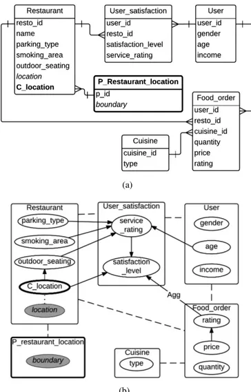
(a)
(b)
Fig. 3: An example of (a) a spatial relational schema adapted
for the spatial attributeRestaurant.location, and (b) a PRM-SA
added spatial reference slots respectively. Then, for each class X ∈ {X ∪ PSA} and each attribute A ∈ {A(X) ∪ CSA(X)}, we have
• a set of parents P a(X.A) = {U1, ..., Ul}, where each Ui
has the form X.B or γ(X.K.B), where B is an attribute of any class, K is a slot chain and γ is an aggregate of X.K.B,
• a legal conditional probability distribution CPD, P (X.A |
P a(X.A)).z
In the relational schema of Fig. 1a, Restaurant is a spatial
class with a spatial geometry attribute location (shown in
italics). To have a PRM-SA defined for this schema, we
adapt it as shown in Fig. 3a, where Restaurant.C location
is the added spatial ref. slot, and refers to the
spa-tial partition class P restaurant location objects defined for
Restaurant.location. The objects of P restaurant location are
de-fined using a spatial partition function, e.g., K-means. In
Fig. 4: Overview of PRM benchmark generation process [14].
attribute, called boundary, which is a polygon, and contains
information about the boundary of the partitions. Since this class is a spatial class, we can further partition the spatial geometry attribute of this class, thereby creating a hierarchy (not shown here). An example of a PRM-SA (structure only) defined for the adapted relational schema is shown in Fig. 3b. Like in PRMs, probabilistic inference is performed on a ground Bayesian network obtained by instantiating a PRM-SA for a given relational skeleton. Here, the skeleton must also include the objects of spatial partition classes.
III. SYNTHETIC DATASET GENERATION WITHPRMS
In our earlier works [14], [15], we had proposed a method for generating PRM benchmarks, which is depicted in Fig. 4. This method involves 3 steps – 1) generation of a random PRM, 2) instantiation of the generated PRM with a random relational skeleton to obtain a GBN, and 3) sampling the GBN to obtain synthetic (non-spatial) datasets. This article is concerned with the experimental evaluation of Steps 2 and 3, and proposes the extension of this method for generating synthetic spatial datasets.
A. Non-spatial dataset generation
In the first step of the method presented in Fig. 4, a random relational schema is created, and a random regular PRM is generated for this relational schema by specifying random dependencies between attributes present in the schema, and assigning random CPDs to each attribute. In the second step, a GBN is generated by instantiating the PRM over a randomly generated relational skeleton. We consider two ways of generating relational skeletons – 1) the one proposed in [25], which generates a relational skeleton with nearly equal number of objects of each class, and 2) another using k-partite graph generation algorithm [15], which generates more realistic skeletons with varying number of objects of each class. Finally, in the third step, a standard sampling algorithm for sampling Bayesian networks is applied on this network to generate a sample, which is then stored in a database. Forward
Sampling[26] is a well-known algorithm for this task. Though
this approach is theoretically possible, it may be impractical when it comes to generate very big datasets because the GBN would be huge for big datasets. Moreover, GBN generation is itself an expensive task.
Algorithm 1: Relational Forward Sampling Input: A PRM, Π =< R, S >; A relational skeleton, σr Output: An instance (or a sample), I
1: G ← Dependency structure of Π in topological order
2: for each node X.A ∈ G do
3: for each object x ∈ σr(X) do
4: if X.A has no parent then
5: Sample x.A from P (X.A) and write to I
6: else
7: e ← {}
8: for X.γ.B ← Parents of X.A do
9: Z.B ← X.γ.B
10: if Aggretation needed then
11: e ← e∪ Aggregate all z.B that have
x.A as their child
12: else
13: e ← e ∪ z.B that has x.A as its child
14: end if
15: end for
16: Sample x.A from P (X.A | e) and write to I
17: end if
18: end for
19: end for
Fig. 5: Generalization of PRM benchmark generation process .
We generalize the PRM benchmark generation process, as shown in Fig. 5, by skipping the specificity of PRM sampling technique to clarify that sampling a GBN is not the only way of generating synthetic datasets from a PRM. Relational forward
sampling(Algorithm 1) aims at sampling a PRM without using
a GBN. It adapts Forward Sampling algorithm for relational context and works directly with databases. This algorithm samples each PRM node in a topological order, and generates a random value for the corresponding attribute of all objects in the skeleton. Because this algorithm does not need to deal with GBN, GBN generation time is saved with this algorithm. The only time consuming operation in this algorithm is the communication with databases.
B. Spatial dataset generation
Synthetic spatial datasets can be generated by following the method of generating non-spatial datasets, and replacing the non-spatial components by their spatial counterparts. That means, we need to generate a PRM-SA (instead of a regular PRM) for a spatial relational schema, and instantiate it over a randomly generated spatial relational skeleton.
1) Random PRM-SA generation: As PRM-SA is defined for
a spatial relational schema adapted for the constituent spatial attributes, we first generate such schema. A spatial relational schema consists of two types of classes – one with spatial attributes, and the other without spatial attributes. The non-spatial part of such schema can be generated by following [14]’s method of generating a relational schema. Now to add spatial components to the generated non-spatial schema, the required number of spatial classes are selected from the schema, and spatial attributes are added to each of them. In the context of spatial databases, these spatial attributes would be columns of type ‘geometry’. For each added spatial attribute, a spatial ref. slot is added to the class, a spatial partition class is introduced to the schema, and a relational link between the spatial ref. slot and the spatial partition class is added. Generating random dependencies among non-spatial, and spatial ref. slots, and assigning random CPDs to each of these nodes will result in a random PRM-SA.
2) Spatial relational skeleton generation: A spatial
rela-tional skeleton can be generated in the same way as its non-spatial counterpart with a special constraint that the skeleton cannot have arbitrary number of partition class objects. For any spatial attribute, the set of objects of associated partition class is the range of the spatial partition function associated with the spatial attribute, and the corresponding spatial ref. slots refer to this set of partition class objects only. In other words, for any spatial partition class, the number of objects cannot exceed the cardinality of the domain of the referring spatial ref. slots. For this reason, we first generate partition class objects, and then generate the non-spatial part of the skeleton. These two operations can be interchanged or be done in parallel as they are independent. Finally, we add links between objects of spatial partition classes and those of respective spatial classes. This process is presented in Algorithm 2.
3) PRM-SA sampling: Sampling a PRM-SA can be
sepa-rated into two tasks, which can be achieved independently, – a) sampling of non-spatial attributes, and b) sampling of spatial attributes.
a) Sampling non-spatial attributes: A spatial relational
skeleton differs from a non-spatial relational skeleton in that some of the attributes are already observed in the former one. Spatial ref. slots, which act as both foreign keys and de-scriptive attributes, are already initialized during the skeleton generation process. Relational forward sampling (see Algo-rithm 1) is not applicable for generating spatial datasets from such partially-observed skeleton because it does not support evidences. Another way to generate a dataset from such par-tially initialized skeleton is to instantiate the PRM-SA over the skeleton to obtain a GBN, set evidences to this network, and
Algorithm 2: Spatial Relational Skeleton Generation Input: A PRM-SA, Π; Total number of objects in the
result-ing skeleton, N ;
Output: A spatial relational skeleton σr
1: G ← DAG representation of the spatial relational Schema
of Π
2: PSA← The set of partition classes in G
3:
4: for P ∈ PSAdo
5: σr(P ) ← Generate objects for P
6: end for
7:
8: G0← {G\PSA} . Sub-DAG obtained by removing
partition classes
9: σ0r← Generate non-spatial relational skeleton(G0, N )
10: σr← σr∪ σ0
r
11: Add links between σr(PSA), and σr(SA) in accordance
with Π
Algorithm 3: Relational Block Gibbs sampling (based on [20]’s LABG algorithm)
Input: A PRM, Π; A relational skeleton, σr, with or without
observations, e; burn-in, N Output: An instance (or a sample), I
1: G ← Generate GBN structure of Π for σr
2: Set evidences if any
3: Sample initial states s(0)
4: for t = 1 to N do
5: s(t)← s(t−1)
6: X.A ← Select an attribute for sampling
7: for each x.A ∈ G(X.A) do
8: if x.A is not observed then
9:
Pφ0(x.A) ← P (x.A | P a(x.A))
Y
y.B∈Ch(x.A)
P (y.B | P a(y.B))
10: Pφ← Normalize(P0
φ)
11: s(t)hx.Ai ← Sample Pφ0(x.A)
12: end if
13: end for
14: end for
then apply a BN sampling algorithm that supports evidences, such as Rejection sampling, Gibbs sampling etc. Alternatively, we can devise relational extensions of other BN sampling algorithms that support evidences.
To avoid the generation of a complete GBN, and to support evidences in relational skeletons, we propose Relational Block Gibbs (RBG) sampling algorithm, presented in Algorithm 3, which is based on [20]’s LABG algorithm. Good points about RBG algorithm are that it can be applied on partially observed skeletons, and it can also support the PRMs that have cycles in class level but are guaranteed to be acyclic in instance level. LABG starts with a partial GBN induced by the query. In our case, the query is the set of all unobserved variables.
This can lead to the generation of a complete GBN (when all attributes are not observed). To avoid this, only the structure of the GBN is generated in our approach; full CPDs are not computed for a couple of reasons because full CPDs are big tables and may require quite a good amount of memory for large and complicated GBNs. Besides, only a small number of values from these CPDs are required during actual sampling of the nodes. So, we compute those values only when required. After generating the structure and setting evidences, an initial sample is generated by assigning random values to unobserved nodes. This structure is imagined to be partitioned into blocks, where each block contains all nodes corresponding to the same attribute X.A. Then, an attribute X.A (or a block) is randomly selected with probability proportional to the size of its block. For each unobserved node in that block, its Markov blanket
is identified to compute full conditional distribution Pφ and
the node is then sampled according to this distribution. The steps of selecting a block and performing Gibbs sampling is performed a finite number of times or until convergence.
b) Sampling spatial attributes: RBG sampling algorithm
is essential for generating spatial datasets from PRM-SA as other existing algorithms cannot deal with partially-observed spatial relational skeleton. However, it samples only non-spatial attributes. To get a complete non-spatial dataset, we need to sample spatial attributes too. Sampling a spatial attribute requires assigning the centers of partitions (i.e., sampling the spatial attribute of spatial partition classes), and then sampling the remaining spatial attributes in the skeleton.
We propose two methods for assigning random partition centers – constrained randomization, and unconstrained ran-domization. In the former method, we pick random points from the entire world and assign them as the center of partitions. If the boundary of partitions is also needed, we can generate random polygons around the centers. In constrained randomization, the input can be a collection of points, a fixed polygon or a collection of polygons. In the first case, where the input is a collection of points, we pick random points from the collection and assign them as centers of partitions. For example, we need to simulate data for some specific cities, we are given a collection of cities as points, and we pick random cities to be the center of partitions. In the second case, where we have to sample spatial attributes from a fixed polygon (e.g., a specific country/city), we divide the polygon randomly into the required number of clusters and pick a random point within the polygons as the center of the partitions. In the last case, where the input is a collection of polygons, we pick random polygons as the boundary of partitions and then pick a random point within the polygon as the center of that partition.
Once we have chosen center and/or boundary of the partition classes, we can proceed with the generation of spatial attributes of spatial classes by generating random points around the centers and within the boundary (if boundary is available) such that the points follow a bivariate normal distribution with the center of the partition as mean and a random positive definite matrix as variance covariance matrix.
IV. EXPERIMENTS
We carried out some experiments to study Relational Block Gibbs (RBG) sampling algorithm, and compare it with Re-lational Forward Sampling (RFS), and sampling on GBN (which we will refer to as GBN-based sampling). These algorithms are implemented in PILGRIM [27], a software library for probabilistic graphical models, being developed at LS2N laboratory. We used the same for these experiments.
We deal with two types of relational skeletons in the experiments – one is generated using [25]’s algorithm, which generates a relational skeleton with nearly equal number of objects of each class, and another using k-partite graph generation algorithm [15], which generates more realistic skeletons with varying number of objects of each class. We refer to relational skeletons generated by the former algorithm as ‘Na¨ıve’ skeletons because they are less complex than the skeletons generated by the latter one. Since the experiments are not concerned with the generation of random PRMs, we use pre-defined PRMs(-SA) for all experiments.
We divide these experiments into two parts. In the first part, we apply RBG sampling algorithm to generate spatial datasets, and study its performance with respect to burn-in, relational skeleton type, and dataset size. In the second part, we compare RFS, RBG, and GBN-based sampling algorithms. Because RFS does not support evidences (a crucial require-ment for sampling PRMs-SA), and also because for GBN-based sampling PILGRIM relies on ProBT [28] library, which does not provide sampling algorithms that support evidences, we generate only non-spatial datasets from these algorithms to compare their performance. Moreover, since these two algorithms are used for sampling non-spatial attributes of SA, it is not necessary to apply them to sample PRMs-SA to compare the performance of these algorithms.
In the following, Section IV-A presents the study of RBG sampling, and Section IV-B presents the comparison of the three algorithms.
A. Empirical study of relational block Gibbs sampling algo-rithm
The aim of this study is to understand how relational block Gibbs sampling algorithm performs on different types of datasets of varying size, and how burn-in value affects the performance of the algorithm.
1) Methodology: We start with a PRM-SA shown in
Fig. 6a. The corresponding relational schema (before adapting for the PRM-SA) is shown as a DAG in Fig. 6b. Conforming to the (adapted) relational schema of this PRM-SA, we generate na¨ıve and k-partite graph-based skeletons having approxi-mately 100, 200, 500, 1000, 2000, 3000, and 5000 objects. So, we have altogether 14 relational skeletons. While generating k-partite skeletons, the choice of the scalar parameter α affects the structure of the skeleton to a great extent. Smaller values of α result in compact skeletons, i.e. many objects will have high in-degree. In-degree of objects, in fact, is determined by whether a referring object gets linked to an existing object or a new object, which in turn depends on the total number of
(a)
(b)
Fig. 6: (a) The PRMSA used in the experiments, and (b) the underlying relational schema as a DAG
objects generated so far. Thus, instead of picking a constant α for skeletons of different size, it should be chosen based on the size of the skeleton. In this study, we choose α to be the square root of the required number of objects in the skeleton. Also note that while generating these k-partite skeletons, we choose not to generate true scale-free graphs to avoid getting very complex skeletons for the experiments. Next, the PRM-SA is sampled for each of these skeletons applying RBG sampling algorithm with the following burn-in values – 100, 200, 300, 400, 500, 600, 700, 800, 900, 1000, 1500, 2000, 2500, and 3000. For each combination of dataset size, burn-in and skeleton type, the time taken to complete the algorithm is recorded, and parameters of the PRM-SA are learned on the generated sample. Chi-square goodness-of-fit test with significance level of 0.05 is performed to compare the original parameters with the learned ones. Using this test, we can check how well the PRM-SA nodes are sampled. Null hypothesis of this test is that the generated data for the given node are consistent with the original distributions used for generating the sample. The nodes that reject the test cannot be considered well-sampled. We count such nodes too.
2) Characteristics of the datasets: As mentioned
previ-ously, there are 14 relational skeletons – 7 na¨ıve skeletons, and 7 k-partite skeletons. Note that in terms of the size of the dataset, we consider the na¨ıve skeleton with approximately 100 objects is comparable to the k-partite skeleton with approximately the same number of objects even though we cannot ensure that they have exactly the same number of objects.
In na¨ıve skeletons, objects are almost uniformly distributed across classes as seen from Fig. 7 whereas in k-partite skeletons, the number of objects of relationship classes (i.e.,
Rating,Shot at, andReads) is higher than that of entity classes
book movie users reads rating
Total number of objects = 200
Number of objects 0 10 20 30 40
book movie users reads rating
Total number of objects = 1000
Number of objects
0
50
100
200
book movie users reads rating
Total number of objects = 2000
Number of objects
0
100
300
book movie users reads rating
Total number of objects = 3000
Number of objects
0
200
400
600
book movie users reads rating
Total number of objects = 5000
Number of objects 0 400 800 Naive K-partite
Fig. 7: Distribution of objects in the relational skeletons used in the experiments
(i.e.,Book,Movie, andUser) in almost all cases. However, this
expected phenomenon is not observed in the smaller datasets because the chosen scalar parameter might not have been enough to produce very compact datasets.
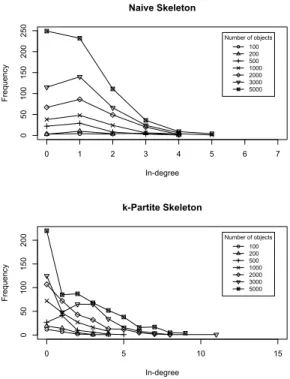
Fig. 8 and Fig. 9 reveal that na¨ıve skeletons are less complex than k-partite graph-based skeletons. The five charts in Fig. 8 correspond to the five edges present in the relational schema DAG shown in Fig. 6b. The charts show that the maximum in-degree of entity objects in na¨ıve skeletons is almost always less than k-partite skeletons, and does not increase significantly with the size of data. Fig. 9 shows the frequency of
in-degree of User objects for the references from Ratingobjects
in the na¨ıve and k-partite skeletons of different sizes. The same phenomenon was observed for other edges (not shown here due to space constraints). In this figure, we can see that there are more objects with high in-degree in k-partite skeletons compared to the corresponding na¨ıve skeletons. From these figures, we can conclude that the experimental k-partite skeletons are complex than the na¨ıve skeletons.
3) Results and discussion: Fig. 10 and Fig. 11 show the
time taken by the sampling algorithm on each skeleton for different values of burn-in. Here, we can see that it took longer to sample on k-partite skeletons than on na¨ıve skeletons. Possible reason behind this is that na¨ıve skeletons are generally simpler than k-partite skeletons because the latter ones tend to have nodes/objects that are referenced by many other nodes. Therefore, Markov blankets in k-partite skeletons tend to be much bigger than those in na¨ıve skeletons, thereby increasing computation time for conditional probability distributions. Another observation we can make is that the time taken by the algorithm increases almost linearly with the burn-in value (and also with the skeleton size). We can only expect to observe such linear relationship but cannot guarantee it because time
0 1000 2000 3000 4000 5000 0 2 4 6 8 User-Reads Dataset size Max in-degree 0 1000 2000 3000 4000 5000 0 5 10 15 Book-Reads Dataset size Max in-degree 0 1000 2000 3000 4000 5000 0 2 4 6 8 User-Rating Dataset size Max in-degree 0 1000 2000 3000 4000 5000 0 2 4 6 8 Movie-Rating Dataset size Max in-degree 0 1000 2000 3000 4000 5000 0 2 4 6 8 Movie-Shot_at Dataset size Max in-degree K-partite Naive
Fig. 8: Max in-degree of entity objects in the relational skeletons. Each chart corresponds to one of the four edges in the relational schema DAG of Fig. 6b
0 1 2 3 4 5 6 7 0 50 100 150 200 250 Naive Skeleton In-degree Frequency Number of objects 100 200 500 1000 2000 3000 5000 0 5 10 15 0 50 100 150 200 k-Partite Skeleton In-degree Frequency Number of objects 100 200 500 1000 2000 3000 5000
Fig. 9: Distribution of in-degree in na¨ıve and k-partite
skele-tons for the edge to User fromRatingobjects
taken for sampling actually depends on which attribute is selected, and how big its Markov blanket is. Because selecting an attribute for sampling and generating attribute values are
0 1000 2000 3000 4000 5000 10 20 30 Number of objects = 100 Burn-in Time taken (s) 0 1000 2000 3000 4000 5000 20 40 60 80 Number of objects = 200 Burn-in Time taken (s) 0 1000 2000 3000 4000 5000 40 100 160 Number of objects = 500 Burn-in Time taken (s) 0 1000 2000 3000 4000 5000 100 250 Number of objects = 1000 Burn-in Time taken (s) 0 1000 2000 3000 4000 5000 200 600 Number of objects = 2000 Burn-in Time taken (s) 0 1000 2000 3000 4000 5000 200 800 1400 Number of objects = 3000 Burn-in Time taken (s) 0 1000 2000 3000 4000 5000 500 2000 Number of objects = 5000 Burn-in Time taken (s) K-partite Naive
Fig. 10: Burn-in vs time taken by RBG sampling algorithm on na¨ıve and k-partite graph-based skeletons of different size.
done randomly, we cannot predict the exact behavior of the increase of burn-in value.
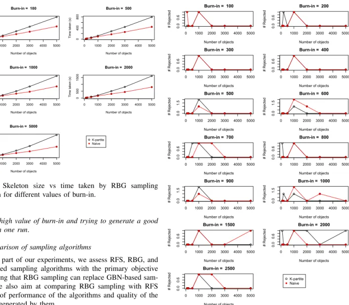
Fig. 12, and Fig. 13 present the number of nodes that rejected the null hypothesis of Chi-squared goodness-of-fit test for different burn-in values on skeletons of different size. No nodes must reject the null hypothesis in a well-sampled dataset. So, lower values are better in these charts. As seen here, out of eight nodes in the PRM-SA, at most two nodes rejected the null hypothesis on both types of skeletons. There is no clear pattern of getting well sampled data as a function of skeleton size. We have cases such as the na¨ıve skeleton with 500 objects being perfectly sampled, that with 1000 objects having at least one rejected node for all values of burn-in, again that with 2000 objects being perfectly sampled for all except one values of burn-in, and exactly the opposite for equivalent k-partite skeletons. From these results, we are indecisive about the size of skeletons and the value of burn-in to get perfect samples. However, we can say that increasing burn-in can improve the quality of samples with the cost of time (cf. Fig. 10). We should note that even small values of burn-in could generate good samples for big datasets (e.g., both na¨ıve, and k-partite skeletons having more than 3000 objects with burn-in < 1000 in Fig. 13). Thus, it would be better to generate big datasets using a small value of burn-in repeatedly until a well-sampled dataset is obtaburn-ined burn-instead
0 1000 2000 3000 4000 5000 0 200 500 Burn-in = 100 Number of objects Time taken (s) 0 1000 2000 3000 4000 5000 0 400 800 Burn-in = 500 Number of objects Time taken (s) 0 1000 2000 3000 4000 5000 0 400 800 Burn-in = 1000 Number of objects Time taken (s) 0 1000 2000 3000 4000 5000 0 500 1500 Burn-in = 2000 Number of objects Time taken (s) 0 1000 2000 3000 4000 5000 0 1500 3000 Burn-in = 5000 Number of objects Time taken (s) K-partite Naive
Fig. 11: Skeleton size vs time taken by RBG sampling algorithm for different values of burn-in.
of using high value of burn-in and trying to generate a good sample in one run.
B. Comparison of sampling algorithms
In this part of our experiments, we assess RFS, RBG, and GBN-based sampling algorithms with the primary objective of verifying that RBG sampling can replace GBN-based sam-pling. We also aim at comparing RBG sampling with RFS in terms of performance of the algorithms and quality of the samples generated by them.
1) Methodology: Because RFS cannot be applied on
PRMs-SA, we use a regular PRM shown in Fig. 14 for this experiment. We first generate na¨ıve and k-partite graph-based skeletons having 100, 200, 500, 1000, 2000, and 3000 objects. The three sampling algorithms are applied over these skeletons to sample the PRM. From the previous experiments (Section IV-A), it was observed that high burn-in values are not necessary for obtaining good samples from big skeletons. That is why we use a medium value (600) of burn-in for RBG sampling in this experiment.
2) Results and discussion: Fig. 15 shows that when the
time taken to complete the sampling algorithms is considered, RFS outperforms the two other sampling algorithms. Even on big datasets, it took very less time compared to the two others. Time efficiency of this algorithm lies behind its non-iterative nature and the fact that GBN generation is not required for it. Unlike RBG sampling, it samples each attribute only once. The only time-consuming task in RFS is the communication with databases. Therefore, we can conclude that RFS is certainly a good solution if we need to generate very big datasets. One important thing to note here is that it is difficult to determine
0 1000 2000 3000 4000 5000 0.0 0.6 Burn-in = 100 Number of objects # Rejected 0 1000 2000 3000 4000 5000 0.0 0.6 Burn-in = 200 Number of objects # Rejected 0 1000 2000 3000 4000 5000 0.0 0.6 Burn-in = 300 Number of objects # Rejected 0 1000 2000 3000 4000 5000 0.0 0.6 Burn-in = 400 Number of objects # Rejected 0 1000 2000 3000 4000 5000 0.0 1.5 Burn-in = 500 Number of objects # Rejected 0 1000 2000 3000 4000 5000 0.0 1.5 Burn-in = 600 Number of objects # Rejected 0 1000 2000 3000 4000 5000 0.0 0.6 Burn-in = 700 Number of objects # Rejected 0 1000 2000 3000 4000 5000 0.0 0.6 Burn-in = 800 Number of objects # Rejected 0 1000 2000 3000 4000 5000 0.0 1.5 Burn-in = 900 Number of objects # Rejected 0 1000 2000 3000 4000 5000 0.0 1.5 Burn-in = 1000 Number of objects # Rejected 0 1000 2000 3000 4000 5000 0.0 0.6 Burn-in = 1500 Number of objects # Rejected 0 1000 2000 3000 4000 5000 0.0 0.6 Burn-in = 2000 Number of objects # Rejected 0 1000 2000 3000 4000 5000 0.0 0.6 Burn-in = 2500 Number of objects # Rejected K-partite Naive
Fig. 12: Skeleton size vs number of nodes that rejected the null hypothesis of the Chi-square goodness-of-fit test for different values of burn-in. Lower values are better here.
the most time-efficient algorithm among RBG and GBN-based sampling because they are sensitive to the complexity of relational skeletons. This sensitivity can be observed in Fig. 15; RBG sampling took longer on k-partite skeletons but not on na¨ıve ones. Moreover, RBG sampling also depends on the value of burn-in as well as on the time of execution. If we had chosen a smaller burn-in value, we might have obtained very different results. Because attributes are selected randomly for sampling at each step, no two executions of RBG sampling for the same burn-in value would give the same result.
We can observe in Fig. 16 that the number of the nodes rejecting the null hypothesis of the Chi-squared goodness-of-fit test is always lower for RBG sampling on both types of skeletons. All six nodes in the PRM were sampled well on k-partite skeletons by RBG sampling except in one case where only one node rejected the null hypothesis. Also on naive
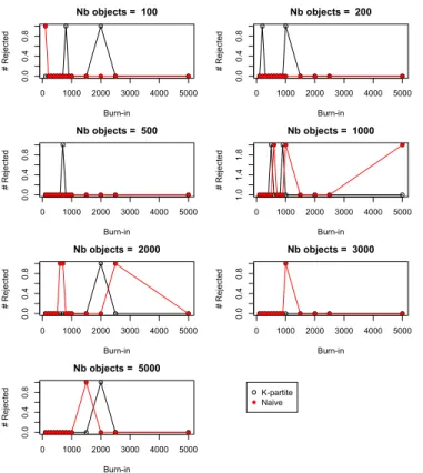
0 1000 2000 3000 4000 5000 0.0 0.4 0.8 Nb objects = 100 Burn-in # Rejected 0 1000 2000 3000 4000 5000 0.0 0.4 0.8 Nb objects = 200 Burn-in # Rejected 0 1000 2000 3000 4000 5000 0.0 0.4 0.8 Nb objects = 500 Burn-in # Rejected 0 1000 2000 3000 4000 5000 1.0 1.4 1.8 Nb objects = 1000 Burn-in # Rejected 0 1000 2000 3000 4000 5000 0.0 0.4 0.8 Nb objects = 2000 Burn-in # Rejected 0 1000 2000 3000 4000 5000 0.0 0.4 0.8 Nb objects = 3000 Burn-in # Rejected 0 1000 2000 3000 4000 5000 0.0 0.4 0.8 Nb objects = 5000 Burn-in # Rejected K-partite Naive
Fig. 13: Burn-in vs number of nodes that rejected the null hypothesis of the Chi-square goodness-of-fit test on k-partite graph-based skeletons, and na¨ıve skeletons of different size. Lower values are better here.
Fig. 14: The PRM used for comparing sampling algorithms
skeletons, the best result was obtained with RBG sampling. Though RFS was very efficient in terms of time, at least one node was not well sampled with this algorithm. From these observations, we can conclude that nodes are generally sampled well with RBG sampling even though it is slower than RFS.
V. CONCLUSION
Having real datasets for evaluating data mining or machine learning algorithms can be difficult, for example, due to legal issues or system complexities. In such case, synthetic or artificial datasets are often used. This practice is quite common in both spatial and non-spatial context. Most techniques for generating synthetic datasets are oriented towards generation
0 500 1000 1500 2000 2500 3000 0 2000 4000 6000 K-partite Number of objects Time taken (s) 0 500 1000 1500 2000 2500 3000 0 500 1000 1500 Naive Number of objects Time taken (s) RFS RBG GBN-based
Fig. 15: Time taken by RFS, RBG, and GBN-based sampling algorithms on na¨ıve and k-partite graph-based skeletons of different size.
Number of objects
# nodes that reject H0
0.0 0.5 1.0 1.5 2.0 100 200 500 1000 2000 3000 KPARTITE 100 200 500 1000 2000 3000 NAIVE RFS GBN-based RBG
Fig. 16: Number of nodes that rejected the null hypothesis of the Chi-square goodness-of-fit test on na¨ıve and k-partite graph-based skeletons of different size. Lower values are better here.
of flat (non-relational) datasets whereas most tools dealing with the generation of relational datasets generate random values for object attributes without considering regularities in the data, an essential aspect of data required for evaluating data mining algorithms. In this article, we have tried to address this problem through our approach of using Probabilistic Relational Models (PRMs) to generate synthetic spatial and non-spatial relational databases. This is an extension to our previous works [14], [15] in the same direction, where the objective was to generate non-spatial relational databases using
PRMs for evaluating PRM learning algorithms. Our approach of generating synthetic spatial databases uses PRMs with Spatial Attributes (PRMs-SA), an extension of regular PRMs, that support spatial information.
Our method of generating synthetic data involves 3 steps -1) generating a random PRM, 2) generating an instance of a relational schema, called relational skeleton, and 3) applying a sampling algorithm on the PRM over the generated skeleton to generate a dataset. We performed experiments concerning mainly Steps 2, and 3. We used 2 different types of relational skeletons, and applied 3 sampling algorithms over them - i) sampling on a GBN (GBN-based sampling), ii) Relational Forward Sampling (RFS), and iii) Relational Block Gibbs (RBG) Sampling. As our conclusion of these experiments, we present the following guidelines for those who are interested in using PRMs for generating synthetic datasets.
1) To generate very big non-spatial datasets, RFS would be the best choice even though the generated dataset may not be as well sampled as with RBG sampling algorithm because RFS is very time-efficient regardless of the complexity of dataset structure (or relational skeleton). 2) So far, only RBG, and GBN-based sampling algorithms
have been studied for generation of spatial datasets. 3) If the quality of datasets is high priority, then the best
option is RBG sampling algorithm. However, one should be aware that the execution time for this algorithm varies greatly with the size/complexity of the relational skeleton, and that the quality of the generated datasets depends on the burn-in values. From our experimental results, we suggest the use of small values of burn-in, and, if necessary, the repeated application of RBG to obtain well sampled datasets.
4) In our experiments, GBN-based sampling algorithm was not found to be as fast as RFS, and did not produce datasets as good as the ones generated by RBG algo-rithm. However, we should not label it as the worst algorithm. It can be interesting to apply GBN-based sampling in the case when RBG is too slow (i.e., when relational skeleton is too complex or big) to generate spatial datasets (i.e., when RFS is not applicable). Our future perspective is to provide our work presented here as a software, which would help the communities inter-ested in generating synthetic spatial and non-spatial relational databases using PRMs.
REFERENCES
[1] DataFiller. [Online]. Available:
https://www.cri.ensmp.fr/people/coelho/datafiller.html [2] ObjectFiller.NET. [Online]. Available: http://objectfiller.net/ [3] Generate data. [Online]. Available: http://www.generatedata.com/ [4] Faker. [Online]. Available: https://github.com/fzaninotto/Faker [5] K. Kennedy, S. J. Delany, and B. Mac Namee, “A framework for
generating data to simulate application scoring,” 2011.
[6] H. Christiansen and C. M. Dahmcke, “A machine learning approach to test data generation: A case study in evaluation of gene finders,” in International Workshop on Machine Learning and Data Mining in
Pattern Recognition. Springer, 2007, pp. 742–755.
[7] R. P. Lippmann, D. J. Fried, I. Graf, J. W. Haines, K. R. Kendall, D. Mc-Clung, D. Weber, S. E. Webster, D. Wyschogrod, R. K. Cunningham et al., “Evaluating intrusion detection systems: The 1998 DARPA off-line intrusion detection evaluation,” in DARPA Information Survivability Conference and Exposition, 2000. DISCEX’00. Proceedings, vol. 2. IEEE, 2000, pp. 12–26.
[8] R. A. Hazwani, N. Wahida, S. I. Shafikah, P. N. Ellyza et al., “Automatic artificial data generator: Framework and implementation,” in Information and Communication Technology (ICICTM), International Conference
on. IEEE, 2016, pp. 56–60.
[9] P. D. Scott and E. Wilkins, “Evaluating data mining procedures: tech-niques for generating artificial data sets,” Information and software technology, vol. 41, no. 9, pp. 579–587, 1999.
[10] K. Hermes and M. Poulsen, “A review of current methods to generate synthetic spatial microdata using reweighting and future directions,” Computers, Environment and Urban Systems, vol. 36, no. 4, pp. 281– 290, 2012.
[11] J. Pearl, Probabilistic Reasoning in Intelligent Systems: Networks of
Plausible Inference. San Francisco, CA, USA: Morgan Kaufmann
Publishers Inc., 1988.
[12] N. Friedman, L. Getoor, D. Koller, and A. Pfeffer, “Learning probabilis-tic relational models,” in International Joint Conference on Artificial
Intelligence, vol. 16. Lawrence Erlbaum Associates Ltd, 1999, pp.
1300–1309.
[13] L. Getoor, N. Friedman, D. Koller, A. Pfeffer, and B. Taskar, “Probabilis-tic relational models,” in Introduction to statis“Probabilis-tical relational learning, L. Getoor and B. Taskar, Eds. The MIT press, 2007, ch. 5, pp. 129–174. [14] M. Ben Ishak, P. Leray, and N. Ben Amor, “Probabilistic relational model benchmark generation: Principle and application,” Intelligent Data Analysis, vol. 20, no. 3, pp. 615–635, 2016.
[15] M. Ben Ishak, R. Chulyadyo, and P. Leray, “Probabilistic Relational Model Benchmark Generation,” LARODEC Laboratory, ISG, Universit´e de Tunis, Tunisia ; DUKe research group, LINA Laboratory UMR 6241, University of Nantes, France ; DataForPeople, Nantes, France, Technical Report, Feb. 2016.
[16] R. Chulyadyo and P. Leray, “Integrating spatial information into prob-abilistic relational models,” in IEEE International Conference on Data Science and Advanced Analytics, ser. DSAA’15, Paris, France, Oct 2015, pp. 1–8.
[17] L. Getoor, N. Friedman, D. Koller, and B. Taskar, “Learning proba-bilistic models of relational structure,” in Proceedings of the Eighteenth
International Conference on Machine Learning, ser. ICML ’01. San
Francisco, CA, USA: Morgan Kaufmann Publishers Inc., 2001, pp. 170– 177.
[18] L. Getoor, “Learning statistical models from relational data,” Ph.D. dissertation, Stanford University, 2002.
[19] A. J. Pfeffer, “Probabilistic reasoning for complex systems,” Ph.D. dissertation, Stanford University, 2000.
[20] F. Kaelin, “Approximate Inference in Probabilistic Relational Models,” McGill University, Montreal, Canada, Tech. Rep., 2011.
[21] P.-H. Wuillemin and L. Torti, “Structured probabilistic inference,” Inter-national Journal of Approximate Reasoning, vol. 53, no. 7, pp. 946–968, 2012.
[22] J. Kisynski and D. Poole, “Lifted aggregation in directed first-order probabilistic models.” in Proceedings of the 21st International Joint Conference on Artificial Intelligence, ser. IJCAI 2009, Pasadena, Cali-fornia, USA, 2009, pp. 1922–1929.
[23] B. Milch, L. S. Zettlemoyer, K. Kersting, M. Haimes, and L. P. Kaelbling, “Lifted probabilistic inference with counting formulas.” in Proceedings of the Twenty-Third AAAI Conference on Artificial
Intel-ligence, ser. AAAI 2008, D. Fox and C. P. Gomes, Eds. Chicago,
Illinois, USA: AAAI Press, 2008, pp. 1062–1068.
[24] P. Singla and P. M. Domingos, “Lifted first-order belief propagation.” in AAAI, vol. 8, 2008, pp. 1094–1099.
[25] M. Ben Ishak, “Probabilistic relational models: learning and evaluation,” Ph.D. dissertation, Universit´e de Nantes; Universit´e de Tunis, Institut Sup´erieur de Gestion de Tunis, 2015.
[26] M. Henrion, “Propagating uncertainty in bayesian networks by prob-abilistic logic sampling,” in Uncertainty in Artificial Intelligence, ser. Machine Intelligence and Pattern Recognition, J. F. Lemmer and L. N.
Kanal, Eds. North-Holland, 1988, vol. 5, pp. 149 – 163.
[27] PILGRIM. [Online]. Available: http://pilgrim.univ-nantes.fr/
![Fig. 4: Overview of PRM benchmark generation process [14].](https://thumb-eu.123doks.com/thumbv2/123doknet/12207767.316527/6.918.466.845.101.666/fig-overview-prm-benchmark-generation-process.webp)