HAL Id: hal-02056788
https://hal.archives-ouvertes.fr/hal-02056788
Submitted on 4 Mar 2019
HAL is a multi-disciplinary open access
archive for the deposit and dissemination of
sci-entific research documents, whether they are
pub-lished or not. The documents may come from
teaching and research institutions in France or
abroad, or from public or private research centers.
L’archive ouverte pluridisciplinaire HAL, est
destinée au dépôt et à la diffusion de documents
scientifiques de niveau recherche, publiés ou non,
émanant des établissements d’enseignement et de
recherche français ou étrangers, des laboratoires
publics ou privés.
Efficient Optimization of the Ambiguity Functions of
Multi-Static Radar Waveforms
Fabien Arlery, Rami Kassab, U. Tan, Frederic Lehmann
To cite this version:
Fabien Arlery, Rami Kassab, U. Tan, Frederic Lehmann. Efficient Optimization of the Ambiguity
Functions of Multi-Static Radar Waveforms. 2016 17th International Radar Symposium (IRS), May
2016, Krakow, Poland. pp.1-6. �hal-02056788�
an author's https://oatao.univ-toulouse.fr/22875
http://doi.org/10.1109/IRS.2016.7738627
Arlery, Fabien and Kassab, Rami and Tan, U. and Lehmann, Frédéric Efficient Optimization of the Ambiguity
Functions of MultiStatic Radar Waveforms. (2016) In: 2016 17th International Radar Symposium (IRS), 10 May 2016 -12 May 2016 (Krakow, Poland).
II. NOTATIONS
First, define a family set of complex sequences of length N, with
and its Doppler shift version
where and corresponds respectively to the Doppler shift and the bit time. is supposed to be a predefined waveform envelope (i.e. of constant modulus or pulsed etc.).
If we define a normalized Doppler shift ! such that
"
then can be expressed as " # %$& .
According to that, the correlation of and '", expressed
as ( '" ) '", is given by: * '" + , ) '"-.
0 )' 1 +
" (1)
One important feature of this function is:
* '" + * ' 2" 3+ ". 4 5! 67 89:;6<=6> ! ? @ <AB:;C6D: (2) Now let us define the partial cost function term from which we calculate the gradient:
E '" 0 F* '" + F GH '" .
2
. 2 I
(3) where the exponent J allows some control over the sidelobe level. When J K , E '" corresponds to the weighted integrated sidelobe level (WISL). Otherwise, the larger the exponent, the more emphasized the dominant term is, so the gradient will essentially indicate the gradient of the PSLR. The coefficients H '" . control the shape of the correlation sidelobes (H '" . ? L)in the area of interest and M outside). This partial cost function term is related to the sidelobe energy within the correlation product of and '". It corresponds to the cross-correlation between the NOP sequence and the NQOP sequence with a normalized Doppler shift !.
If we call R the set of Doppler frequencies to optimize such that:
R !S ! ? @ 67 9:;6<=6> ! ? L <AB:;C6D: (4) We can define the cost function related to sidelobe energy within the ambiguity function between and ' within the area of interest, as:
E ' 0 E '"
"?R (5)
From that, the global cost function term from which we calculate the gradient can be expressed as the sum on E ' for each combination of sequences:
E 0 0 E '
T
'
T
(6)
III. GRADIENT METHOD FOR LOCALLY OPTIMIZING THE
AMBIGUITY FUNCTIONS OF A SET OF SEQUENCES
This section provides the gradient of the global cost function, E, related to the sidelobe energy within the auto-ambiguity and cross-auto-ambiguity functions of a set of complex sequences. For calculating this ‘global’ gradient this section is divided in three parts. The first one gives the gradient equation of the cost function associated to the auto-ambiguity function of a sequence. The second part deals with the gradient calculations of the cost function within the cross-ambiguity function of a pair of sequences. And the last one combines the two previous parts and gives the ‘global’ gradient expression.
A. Optimization of the Auto-Ambiguity Function of a Sequence
This subsection provides the gradient of the cost function associated to the auto-ambiguity function of a sequence. The derivations for calculating this gradient has been done in a recent paper [7]. Therefore, for understanding and completeness, this part focuses on the key points of this calculation.
Consider the NOP -sequence of the family, the auto-ambiguity cost function is defined as:
E 0 E "
"?R (7)
where we recall that:
E " 0 F* " + F GH " . 2
. 2 I
(8) One can observe that the gradient of E consists of the sum of the partial gradients E " where E " corresponds to the cost function related to the sidelobe energy within the matched filtering response in presence of a Doppler !.
From that observation, as is a complex sequence with a predefined envelope, the partial gradient is the derivative of the cost function E " with respect to its phase: UEN N !
UVN W .
For clarity, thereafter, E " E" , * " + *" + , H " . H" . and
So, using the chain rule, it can be observed that the derivative with respect to the phase of can be done by calculating the derivatives with respect to the real and imaginary parts of :
UE! UVW 3XN W UE! UY W 1 Y W UE! UXN W (9) As: UE" U Z [J 0 \. "]Y ^*" + _UY ^*U Z" + _ 2 . 2 I 1 XN ^*" + _UXN ^*U Z" + _` (10)
where \" . H" .F*" + F G2 and U Z 4UY a UXN a
The partial derivatives with respect to Y a and XN a are given above ((11) and (12)).
Putting (11) and (12) in the chain rule equation (10) gives the equation (13).
And by defining b" c\. "d. 2 I2 and e" 4 2 f$%g
. , (13) becomes: UE" UVa 3[JXN h W i^,b"j (2" ( - ) , j e"-_ a 1 ^,b"j ("- ) , j e")-(_ I 2akl (14)
Where m( n o 1 K 3 + . is the reverse of m; and j p is the Hadamard product of and p.
Then, by setting: q" #^,b"j (2"( - ) , j e"-_a1 ^,b"j ("- ) , j e")-(_ I 2a& a (15) r" 4UE" UVaga (16)
The previous equation (14) can be converted to a vector form: r" 3[JXNs j q
"t (17)
Therefore by defining: r 4uvu wga , and by taking back the original notation: r " r",
it comes from (7):
r 0 r "
"?R (22)
Finally the gradient can be expressed as a sum of correlation products that can be efficiently computed using Fast Fourier Transform (FFT). If we denote by x y the discrete Fourier Transform operation, and according to our definition of the convolution (1) it can be derived that the convolution of two sequences m and z is equivalent to
[8]
:m ) z x2 , x m x z() - (23)
That gives a computation of r in { o|<}o operations.
B. Optimization of the Cross-Ambiguity Function between a Pair of Sequences
Consider now the gradient calculations of the cost function associated to the cross-ambiguity function of a pair of sequences. Here again this part still focuses on the key points of the calculation (see [7] and [9] for more details)
Let us start with the cross-ambiguity cost function between the NOP -sequence and the NQOP -sequence of the family (N ~ NQ):
E ' 0 E '"
"?R (24)
where we recall that:
E '" 0 F* '" + F GH '" .
2
. 2 I
(25) Similarly to the previous subsection, as (resp. ' is a UE" UY a [J 0 \. "€Y ^*" + _ •Y • W 1 + 2 a"‚ 1 Y • W 3 + a2. "‚‚ 2 . 2 I 1 XN ^*" + _ •3XN • W 1 + 2 a" ‚ 1 XN • W 3 + a2. "‚‚ƒ (11) UE" UXN a [J 0 \. "€Y ^*" + _ •XN • W 1 + 2 a"‚ 1 XN • W 3 + a2. "‚‚ 2 . 2 I 1 XN ^*" + _ •Y • W 1 + 2 a" ‚ 3 Y • W 3 + a2. "‚‚ƒ (12) UE" UVa 3[JXN „ W … 0 \. "*2" 3+ • W 1 + 2 aI. "‚)1 0 \ . "*" + • W 3 + a2. " ‚) 2 . 2 I 2 . 2 I †‡ (13) UE '" UY , W - [J 0 \ '" .Y •* '" + ' W 1 + 2 a" ‚ 2 . 2 I (18) UE '" UXN, W - [J 0 \ '" .XN •* '" + ' W 1 + 2 a" ‚ 2 . 2 I (19) UE '" UY , ' W - [J 0 \ '" .Y ˆ* '" + • W 3 + a2. " ‚)‰ 2 . 2 I (20) UE '" UXN, ' W - 3[J 0 \ '" .XN ˆ* '" + • W 3 + a2. " ‚)‰ 2 . 2 I (21)
complex sequence with a predefined envelope, the partial gradient is the derivative of the cost function E '" with respect to its phase: UEN NŠ !
UVN W (resp. uv ' $
u ' w .
According to the chain rule equation again, we focus our attention to the partial derivatives with respect to Y , a- and XN, a- (resp. Y , 'a- and XN, 'a- and we obtain equations (18) and (19) (resp. (20) and (21)), where \ '" . H '" .F* '" + F G2 .
Putting (18) and (19) (resp. (20) and (21)) in the chain rule equation (10) gives (26) (resp. (27)).
And by defining b '" c\ '" .d
. 2 I 2
and e" 4 2 f$%g
. , equations (26) and (27) become:
UE '" UV W 3[JXN € W •^b '"j ((' 2"_ ) , 'j e"-‚ aƒ (28) UE '" UV ' W 3[JXN i ' W ^,b '"j ( '" -) , 'j e")-(_ I 2ak (29) By noting: r '" 4uvu ' $a g a , r ' '" 4uvu '' $a g a , q‹ '" 4•^b '"j ((' 2"_ ) , 'j e"-‚ aga , qŒ '" #^,b '"j ( '"- ) , 'j e")-(_ I 2a&a ,
the previous equations can be converted to a vector form: r '" 3[JXNi j q‹ '"k (30) r ' '" 3[JXNi 'j qŒ '"k (31) And by defining: r ' 4uvu ' wga and: r ' ' 4uvu ' ' wga it comes from equation (7):
r ' 0 r '"
"?R (32)
r ' ' 0 r ' '"
"?R (33)
Similarly to the previous section, the gradient consists of a sum of correlation products that can be efficiently computed using Fast Fourier Transforms (FFT) [8].
So the computation of r 'and r ' ' can be done in { o•Ž•o operations.
C. Global Gradient Calculations
From that, the two previous subsections are combined for calculating de ‘global’ gradient.
Given that: E 0 0 E T T (34) It comes: UE UV W 0 0 UEUV W T T (35)
Finally, converted in vector form the equation (35) becomes:
r 0 0 r T T 0 r ' T ' '• 1 0 r ' T ' '• 1 r (36) where: r #u uva& a .
IV. GRADIENT METHOD FOR CONTROLING THE OUT-OF-BAND
FREQUENCIES
This section provides the gradient of the cost function related to the out-of-band spectrum energy of a sequence.
First, define a complex sequence , and its Fourier transform ‘’ “” ! " •’2 over o’ – o elements (zero-padding).
“” ! 0 + 2 ."’
’2
. •
(37) If we define the out-of-band spectrum energy as the cost function term to minimize, it comes:
EQ 0F“” ! F G' ’2 " • H"Q (38) UE '" UV W 3[JXN „ W 0 \ '" .* ' 2" 3+ • ' W 1 + 2 aI. " ‚) 2 . 2 I ‡ (26) UE '" UV ' W 3[JXN „ ' W 0 \ '" .* '" + • W 3 + a2. " ‚) 2 . 2 I ‡ (27)
where H"Q control the shape of the out-of-band emissions (the area of interest).
Similarly to the previous section, as is a complex sequence with a predefined envelope, the gradient is the derivative of the out-of-band cost function EQ with respect to its phase: uuv'
w. Following the same approach as the one described in the previous section, the gradient is given by:
UEQ UVa 3[J QXN ] W 0 \ "“”) ! 2 a" ’ ’2 " • ` (39) where: \"Q H"QF“” ! F ,G'2 -. By defining bQ c\"Qd" 2 I2 , ‘’ “” ! " •’2 , and x’ y
the Discrete Fourier Transform (DFT) over o’ elements, it comes that the gradient vector, rQ #uvu '
w&a is given by: rQ 3[JQXNs j x’,bQj ‘’)-t (40)
Here again, it is obvious that the computation of rQcan be done in { o|<}o operations.
V. APPLICATIONS
This section provides some applications of those methods such as:
- The design of a set of sequences that optimizes the ambiguity functions in aperiodic and periodic case. - And the design of a set of sequences that optimizes
both the ambiguity functions and the out-of-band spectrum rejection in aperiodic and periodic case.
A. Optimizing the ambiguity functions of a set of polyphase sequences
The following examples show the sidelobe rejection that can be obtained by an iterative application of (36).
A random family of complex sequences is generated as a starting point for the algorithm. Then a gradient descent is done by simply adjusting the descent step — during the process. The process continues until an exit criterion is met (an upper limit on the number of iterations, or a lower threshold on the minimum improvement acceptable between two successive iterations).
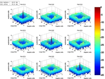
Figures (2), (3), (4) and (5) show the improvement after optimizing the ambiguity functions (R ˜3™š ™›) of a set of ™ complex sequences (of length o KM[œ) in different configurations:
- with a local weighting ( H '. " K W S+S • žœ ŽŸ *HW¡ M 5 ! N NQ );
- with a constant weighting (H '. " K 5 + ! N NQ );
with a large exponent (J œ ) and in both aperiodic and periodic case.
Figure 2. Ambiguity functions obtained with a local weighting in the periodic case.
Figure 3. Ambiguity functions obtained with a local weighting in the aperiodic case.
Figure 4. Ambiguity functions obtained with a constant weighting in the periodic case.
Figure 5. Ambiguity functions obtained with a constant weighting in the aperiodic case.
The algorithm well-improves the PSLR in the area of interest. For comparison, the PSLR of a sequence from the Small Set of Kasami is about [¢£o , i.e. about 3[œ ¤¥ for a sequence of 1024 elements [4]. So even compared to those easily-constructed sequences, it gives better results.
Moreover, this algorithm is highly faster than the cyclic algorithms introduced in [5]. This is due to the efficient gradient calculations ({ o•<}o ) whereas cyclic algorithms are based on a SVD operation (O(N3)) on each iteration.
Figure 6. Ambiguity functions obtained with a local weighting in the aperiodic case.
Figure 7. Spectrums obtained with local weighting in the aperiodic case.
B. Optimizing both the ambiguity functions of a set of polyphase sequences and the out-of-band rejection
This example shows the sidelobe and out-of-band rejections possible by iterative application of (36) and (40). Here, we follow the same process as the one described in the previous examples. Except that in this case, the gradient is given by ¦r 1 K 3 ¦ rQ , where rQ is the out-of-band gradient
vector of the NOP-sequence (Cf. (40)) and ¦ ? §Mš K¨.
Figures (6) and (7) show the result of the optimization in the following configuration: ™ , o KM[œ , R ˜3™š ™› , H '. " K W S+S • žœ <therwise M 5 ! N NQ , J œ , o’ [o [Mœ© , H"Q K W ! ª o <AB:;C6D: M , JQ œ , in
the aperiodic case.
It can be observed that the algorithm still improves the PSLR. The gain may be lower than in the previous case, but, the spectrum is here controlled.
VI. CONCLUSION
In this paper, new gradient methods for optimizing the ambiguity functions of a set of complex sequences were derived.
We have shown that the gradient for optimizing the ambiguity functions is based on simple operations that can be performed using FFT. The result is that the gradient can be computed with O(Nlog(N)) operations. This important result offers the possibility to optimize quite long sequences with relatively a short time of computation compared to existing methods. We have also shown that the gradient for optimizing the out-of-band emissions of a complex sequences is based on DFT operations, that can be fast computed by means of FFT. Finally, by combining both gradients we have designed a set of sequences with interesting properties for radar applications: a low PSLR and a good out-of-band rejection.
REFERENCES
[1] «Surveillance developments in SESAR»
(https://www.eurocontrol.int/articles/surveillance-developments-sesar) [2] N. Millet and M. Klein, «Multi Receiver Passive Radar Tracking,» IEEE
Transactions on Aerospace and Electronic Systems, Vol. 27, No. 10,
2012.
[3] F. Arlery, M. Klein and F. Lehmann, «Utilization of Spreading Codes as dedicated waveforms for Active Multi-Static Primary Surveillance Radar,» IEEE Radar Symposium (IRS), pp. 327-332, 2015.
[4] D. V. Sarwate and M. B. Pursley, «Crosscorrelation properties of pseudorandom and related sequences,» Proceeding of the IEEE, vol. 68, pp. 593-619, May 1980.
[5] H. He, J. Li and P. Stoica, «Waveform Design for Active Sensing Systems : A Computational Approach,» New York: Cambridge University Press, 2012.
[6] J. M. Baden, M. S. Davis and L. Schmieder, «Efficient Energy Gradient Calculations for Binary and Complex Sequences,» IEEE Radar
Conference (RadarCon), pp. 301-309, Mai 2015.
[7] F. Arlery, R. Kassab, U. Tan and F. Lehmann, «Efficient Gradient Method for Locally Optimizing the Periodic/Aperiodic Ambiguity Function,» IEEE Radar Conference (RadarCon), , 2015. ‘in press’ [8] R. N. Bracewell, «The Fourier Transform and its Applications,» 3rd
Edition éd., New York: McGraw-Hill, 1986.
[9] U. Tan, C. Adnet, O. Rabaste, J.-P. Ovarlez and J.-P. Guyvarch, «Phase Code Optimization for coherent MIMO Radar via Gradient Descent,»