HAL Id: hal-01506218
https://hal-mines-paristech.archives-ouvertes.fr/hal-01506218
Submitted on 13 Apr 2017
HAL is a multi-disciplinary open access
archive for the deposit and dissemination of
sci-entific research documents, whether they are
pub-lished or not. The documents may come from
teaching and research institutions in France or
abroad, or from public or private research centers.
L’archive ouverte pluridisciplinaire HAL, est
destinée au dépôt et à la diffusion de documents
scientifiques de niveau recherche, publiés ou non,
émanant des établissements d’enseignement et de
recherche français ou étrangers, des laboratoires
publics ou privés.
Evolution of electrical distribution grid sizing
considering self-consumption of local renewable
production
Antoine Rogeau, Thibaut Barbier, Robin Girard, Nicolas Kong
To cite this version:
Antoine Rogeau, Thibaut Barbier, Robin Girard, Nicolas Kong. Evolution of electrical distribution
grid sizing considering self-consumption of local renewable production. CIRED 2017 - 24th
Inter-national Conference on Electricity Distribution, Jun 2017, Glasgow, United Kingdom. pp. 1248.
�hal-01506218�
EVOLUTION OF ELECTRICAL DISTRIBUTION GRID SIZING
CONSIDERING SELF-CONSUMPTION OF LOCAL RENEWABLE PRODUCTION
Antoine ROGEAU Thibaut BARBIER Nicolas KONG MINES ParisTech – France Robin GIRARD Enedis - France antoine.rogeau@mines-paristech.fr MINES ParisTech – France nicolas.kong@enedis.fr
robin.girard@mines-paristech.fr thibaut.barbier@mines-paristech.fr
ABSTRACT
In the last decades, renewable energy sources have been increasing their shares in the world energy market. In addition to the ecological benefits, this trend can have adjunct benefits, for example for distribution system operators: a gain in their grid sizing. Indeed, installation of decentralized production, when used in a self-consumption approach, can lead to reduction of the self-consumption peaks. This work is willing to quantify what grid sizing reduction a distribution system operator can expect, knowing the renewable energies penetration rate on a MV feeder. To do so, a description of the actual sizing strategy is first described. Estimation of electricity demand is performed using a bottom-up simulation method while photovoltaics and wind power production are evaluated with reanalysis data coupled with a new method to inject variability to the smooth curves. This procedure leads to a new sizing power which can be used, guaranteeing an equivalent quality of supply for consumers. For the tested MV feeders, a maximum reduction of about 4 % of the sizing power is observed. Lastly, an analysis of the under-sizing risk is carried out, characterizing the error in the new sizing power estimation with the number of scenarios taken into account.
INTRODUCTION
Electricity production is a significant source of CO2 emissions. According to the International Energy Agency, in 2013, electricity and heat represented 42% of global CO2 emissions. To tackle this problem, many states are developing energy transition strategies including the growth of renewable energy sources (RES) production. In the case of photovoltaic production, the world cumulative installed capacity targeted by the energy transition roadmap for 2020 is now likely to be achieved five years earlier, and the capacity now expected in 2020 will be over twice that foreseen in the 2010 roadmap [1]. About half of PV deployment is due to be situated on buildings or nearby (such as parking lots) [1].
This implies considerable changes in the planning operation process of the distribution grid. Distribution system operators (DSOs) perform network sizing calculations by distribution considering extreme situations [2]. However, these extreme situations are a combination of different complex dynamics of production and consumer demand. Planning models need to incorporate simulations of these dynamics at local scale. To address this issue, this paper proposes a method for sizing the grid using a bottom-up model of electricity demand and a renewable production load curve simulator. To simulate more realistic production load curves, we present two methods to simulate local weather variability for wind and solar production. Finally, we describe a case study using French main DSO Enedis data.
1. GRID SIZING STRATEGIES AND FREQUENCY OF EXCEEDANCE
Distribution grid sizing calculations are generally carried out when new clients (producers or consumers) opt to connect their installation to the electrical grid. The DSO (e.g. Enedis in France) then verifies whether existing infrastructures, e.g. a distribution station, can handle this new client.
To evaluate the distribution grid’s capacity to receive a new load, Enedis [3] defines dimensioning events that the grid needs to be able to resist. In this paper, we do not consider voltage issues and only consider the three following sizing events:
1) 𝑃𝑃𝑡𝑡𝑡𝑡𝑡𝑡: sizing the grid in normal conditions to resist the load at very low temperature
2) 𝑃𝑃𝑡𝑡𝑚𝑚𝑚𝑚∗ : sizing the grid in incident conditions, by summing the peak demand of all loads at normal temperature
3) 𝑃𝑃𝑝𝑝𝑝𝑝𝑝𝑝𝑝𝑝∗ = 𝑃𝑃𝑝𝑝𝑝𝑝𝑝𝑝𝑝𝑝− 0.2 × 𝑃𝑃𝑡𝑡𝑚𝑚𝑚𝑚∗ : sizing the grid by production. 𝑃𝑃𝑝𝑝𝑝𝑝𝑝𝑝𝑝𝑝 is the RES installed capacity.
The first event describes a case where the grid is at its normal state (no dysfunction), and the temperature is exceptionally low (probability of occurrence 1 day per year). This sizing load is called 𝑃𝑃𝑡𝑡𝑡𝑡𝑡𝑡. The second event considers a situation featuring an accident in the grid, such as a fault in an electric line, and tests the capacity of the restructured grid to resist the load on a normal cold day (the historical mean temperature on 15 January). This load is called 𝑃𝑃𝑡𝑡𝑚𝑚𝑚𝑚∗ . The last strategy is employed when the production means are used to size the grid: the load
considers that all production means generate at their maximum capacity and that consumption is 20% of 𝑃𝑃𝑡𝑡𝑚𝑚𝑚𝑚∗ . The values 𝑃𝑃𝑡𝑡𝑡𝑡𝑡𝑡 and 𝑃𝑃𝑡𝑡𝑚𝑚𝑚𝑚∗ can be calculated in two ways: using Enedis measurements or simulating the load curves.
If we use historical measurements of the load curves, consumer behaviour can be extracted by eliminating the thermosensitive part. This is done by a linear model also used by the French Transmission System Operator [4]. The statistical temperature on 15 January is then applied to the consumer behaviour, using the thermosensitivity model of the historical measurement. We then obtain 𝑃𝑃𝑡𝑡𝑚𝑚𝑚𝑚∗ . The same process, using the temperature with a probability of occurrence of 1/365, extracted from decades of measurements, can be applied to deduce 𝑃𝑃𝑡𝑡𝑡𝑡𝑡𝑡. This method does work, but requires reliable and complete measurement data.
When some data is missing, it may be replaced by simulation. Indeed, Mines ParisTech and Enedis have developed models to simulate electricity demand and production. The electricity demand is highly correlated with the temperature, so introducing the statistical observed temperatures described above as inputs to the model permits to evaluate 𝑃𝑃𝑡𝑡𝑚𝑚𝑚𝑚∗ and 𝑃𝑃𝑡𝑡𝑡𝑡𝑡𝑡.
2. GENERATING CONSUMPTION SCENARIOS
Electricity consumption (power, temporality, etc.) depends on several parameters, such as the weather, solar irradiation and temperature, type of electric device, consumers’ habits and lifestyle, and client category (residential, tertiary, industrial etc.).
For several years, Enedis has been recording the electrical power delivered by its medium voltage (MV) feeders. Each feeder provides electricity for between several hundred and ten thousand low voltage (LV) clients. When Enedis wants to evaluate the impact of an area change on the feeder electricity consumption, different load scenarios are built.
Building these load scenarios relies on two main techniques.
2.1. Using past measurements
One approach consists in using real consumption data. A load curve is available per year, and per MV feeder. It is possible to generate more scenarios from these measurements, by applying the meteorological conditions of an observed year to the consumer behaviour observed in another year. This involves two major steps:
a. Making a thermosensitive model per feeder, and eliminating the thermosensitive part b. Applying another meteorological scenario.
This approach, based on aggregated measured load curves, cannot be employed to simulate new electricity usages, such as electric vehicles or the evolution of household consumption, but only to test different meteorological conditions.
2.2. Using load curve simulation
Another approach is to simulate the load curves according to a given scenario. In our case we use a bottom-up method, named MOSAIC developed by MINES ParisTech and Enedis described in detail in [5]. The description of the different household usages is defined by statistical distributions, thus making it possible to generate different consumption scenarios. The method for generating input data for MOSAIC per MV feeder is described in [3]. Different temperature and irradiation data are used to generate multiple scenarios, combining consumer behaviour and weather conditions in order to provide inputs for MOSAIC.
For each feeder, difficulties exist to collect such data, and for feeders with too many missing values and re-affectations, the past measurement method is not accurate enough. Hence, in the rest of this paper we choose to apply the different sizing methods on a simulated load curve using the MOSAIC method. We likewise calculate the MV feeders 𝑃𝑃𝑡𝑡𝑡𝑡𝑡𝑡 and 𝑃𝑃𝑡𝑡𝑚𝑚𝑚𝑚∗ using the MOSAIC method. Moreover, as MOSAIC is a bottom-up method, it can be used to simulate the load at a smaller scale, such as LV feeders, which are not monitored by Enedis. This downscaling approach using MOSAIC is described and illustrated in [3].
Load curves are simulated using 8 years of meteorological data. Five different scenarios are generated by the MOSAIC method and we thus get 40 possible electricity demand profiles of one year.
3. SIMULATION OF WEATHER VARIABILITY TOWARD REALISTIC RENEWABLE
PRODUCTION DATA
Two local RES are considered in this work: photovoltaics (PV) and wind power (WP). Both productions are estimated from historical weather data, smoothed and sampled at a given temporal and spatial resolution and thus requiring the addition of variability.
3.1. Variability in PV production
Data used to simulate PV production are extracted from the SODA database, which is described in [6]. The spatial resolution of these irradiation data is about 1.5 x 1.5 km and they are sampled at a temporal resolution of
15 minutes. An introduction of spatial variability is performed. The reasoning is based on the fact that if the sky is very cloudy then spatial variability will be low, and this also applies to a very clear sky. However, for a partly cloudy sky, the irradiation variability can be high. For this reason, we performed a study of the error between the SODA irradiance estimation (𝐼𝐼𝑆𝑆𝑆𝑆𝑆𝑆𝑆𝑆) and measured irradiation data (𝐼𝐼𝑆𝑆𝑂𝑂𝑆𝑆) as defined in (1).
𝜀𝜀 =𝐼𝐼𝑆𝑆𝑆𝑆𝑆𝑆𝑆𝑆𝐼𝐼 − 𝐼𝐼𝑆𝑆𝑂𝑂𝑆𝑆
𝑆𝑆𝑆𝑆𝑆𝑆𝑆𝑆 (1)
The analysis is divided into clusters, depending on the Clear-Sky Index 𝐾𝐾𝐶𝐶𝑆𝑆 as defined in [7] estimated at every time step (see (2)).
𝐾𝐾𝐶𝐶𝑆𝑆 =𝐼𝐼𝑆𝑆𝑆𝑆𝑆𝑆𝑆𝑆𝐼𝐼 𝐶𝐶𝑆𝑆
(2)
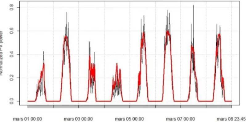
where 𝐼𝐼𝑆𝑆𝑆𝑆𝑆𝑆𝑆𝑆 is the horizontal irradiation given by the SODA model and 𝐼𝐼𝐶𝐶𝑆𝑆 is the horizontal irradiation with a clear sky. The Clear-Sky data are obtained using the ESRA model, described in [8]. This leads us to different error distributions, depending on the cloudiness of the sky. Using the resulting distributions, we added the variability to the initial PV production estimated using SODA data to obtain photovoltaic production estimation, illustrated in Figure 1. This procedure is realized on 8 years data, due to the availability of SODA database. Ten different variable production curves are generated for each year of irradiation data.
Figure 1: Introduction of variability in the PV production. Red: SODA production estimation; Black: Production with variability
3.2. Variability in WP production
Data used to simulate WP production are extracted from the MERRA database, described in [9]. The spatial resolution of these wind data is about 50 km x 50 km and they are sampled at a temporal resolution of 1 hour. We then introduce spatial variability and compare the production estimation obtained using MERRA data with real production measures from several existing wind power plants. This study allows us to estimate wind fluctuations compared to the global trend, representing the slight variations in wind speed and direction. Some studies, such as [10], have shown that the amplitude of fluctuation depends on wind speed, and so we estimate the error between the smoothed curve and the real measures on clusters based on the wind speed. As a result, we obtain production curves with extra variability, as shown in Figure 2.
This procedure is realized on 8 years of data, to be consistent with the solar data availability. Ten different variable production curves are generated for each year of irradiation data.
Figure 2: Introduction of variability in the WP production. Red: MERRA production estimation; Black: Production with variability
4. RESULTS – EVOLUTION OF GRID SIZING
grid sizing of implementing decentralized renewable production. The simulation of these means of production at different penetration rates provides a reliable view of their impact on the aggregated load, and the potential sizing gain in such cases.
Moreover, the risk of misevaluation can be defined, depending on the number of scenarios simulated.
4.1. Evolution of sizing
When integrating renewable production into the grid, this production may possibly reduce demand peaks. It allows a potential gain in grid sizing, also understandable as new clients connected without grid reinforcements, which has been estimated as it follows:
a. Simulation of the original situation, where the feeder is connected only to consumers. A high number of demand scenarios, 2,000 in our case, are generated (different consumption scenarios and meteorological conditions) and a mean overshoot time of 𝑃𝑃𝑡𝑡𝑡𝑡𝑡𝑡 can be estimated.
b. Simulation of scenarios considering decentralized production. A high number of production scenarios (2,000) are generated (different consumption scenarios, meteorological conditions and production variability).
c. Indicators can be estimated for each of the simulations: maximum power flowing through the lines (consumption and production are counted), overshoot time over 𝑃𝑃𝑡𝑡𝑡𝑡𝑡𝑡 and 𝑃𝑃𝑡𝑡𝑚𝑚𝑚𝑚∗ .
d. Estimation of the new sizing power (𝑃𝑃𝑁𝑁𝑁𝑁𝑁𝑁) corresponding to the overshoot time of the original scenario: we obtain the new sizing with the same quality of supply.
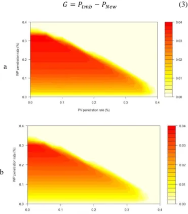
Figure 3 represents the gain in grid sizing (see (3)) depending on the penetration rate of the different RES (in terms of percentage of total contracted power).
𝐺𝐺 = 𝑃𝑃𝑡𝑡𝑡𝑡𝑡𝑡− 𝑃𝑃𝑁𝑁𝑁𝑁𝑁𝑁 (3)
a
b
Figure 3: Evolution of the sizing gain (in % of 𝑃𝑃𝑡𝑡𝑡𝑡𝑡𝑡) depending on the penetration rate. Example of two MV feeders in Lyon, France
This example simulates two MV feeders whose characteristics are detailed in Table 1. Name of feeder “a” “b” Number of clients 2,509 6,982 Total contracted power (MW) 20.25 51.00
𝑃𝑃𝑡𝑡𝑡𝑡𝑡𝑡 (MW) 4.92 12.96
𝑃𝑃𝑡𝑡𝑚𝑚𝑚𝑚∗ (MW) 3.72 9.11
Maximum sizing gain kW 192.93 494.80
%𝑃𝑃𝑡𝑡𝑡𝑡𝑡𝑡 3.92% 3.82%
We can note that both cases show a maximum gain in the grid sizing of about 4 % of 𝑃𝑃𝑡𝑡𝑡𝑡𝑡𝑡. Both MV feeders have a similar behaviour, but the sizing gain is higher for the feeder “a” at the same penetration rate.
WP impact on the gain is considerable while PV production has a very limited – almost inexistent – impact on this sizing gain. This is explained by the fact that PV production is active in the daytime, before sunset, while consumption mainly occurs in the mornings and evenings, when there is no PV production at all. Energy storage could alleviate this effect.
It is also notable that when the installed production power is too high, there is no gain in the grid sizing. Indeed, the maximum power flowing through is mainly due to production, and the grid is sized by production. In the cases presented above, we observe that when the global RES penetration rate (PV+WP) is about over 40%, the grid is sized by production.
4.2. Risks of error
In order to generate the different load and production curves, representing all credible scenarios, the electricity production and demand curves we generated as described in 2. and 3. are sampled. A high amount of simulations are needed to finally obtain an accurate estimation of the most critical case, sizing the grid. For this reason, errors can occur when the number of scenarios simulated is insufficient.
Indeed, in the absence of a very restrictive scenario in the simulations, the new sizing power 𝑃𝑃𝑁𝑁𝑁𝑁𝑁𝑁 elected to ensure the same quality of supply will be underestimated. The real overshoot time corresponding to the new sizing power 𝑃𝑃𝑁𝑁𝑁𝑁𝑁𝑁 will be higher than expected.
The problem can be written as follows:
𝑇𝑇 = 𝑡𝑡���(𝑃𝑃 > 𝑃𝑃𝑁𝑁 𝑡𝑡𝑡𝑡𝑡𝑡) (4)
𝑡𝑡𝑁𝑁
��� represents the time when the load is higher than 𝑃𝑃𝑡𝑡𝑡𝑡𝑡𝑡, averaged over a high number 𝑁𝑁 of scenarios (in our
case, 𝑁𝑁 = 2,000). T can be seen as a given quality of supply. We attempt to quantify 𝜇𝜇𝑖𝑖:
𝜇𝜇𝑖𝑖= 𝑡𝑡���(𝑃𝑃 > 𝑃𝑃𝑁𝑁 𝑖𝑖𝑁𝑁𝑁𝑁𝑁𝑁) (5)
where 𝑃𝑃𝑖𝑖𝑁𝑁𝑁𝑁𝑁𝑁 is the new sizing power, defined using a restricted number of scenarios 𝑛𝑛 such as: 𝑡𝑡� (𝑃𝑃 > 𝑃𝑃𝑛𝑛 𝑖𝑖𝑁𝑁𝑁𝑁𝑁𝑁) = 𝑇𝑇 (6)
𝜇𝜇𝑖𝑖 can thus be seen as extra minutes of overshoot, which are for seen by the client as a quality of supply loss.
The final error is expressed as follows:
𝜀𝜀𝑡𝑡= �𝐾𝐾 �(𝜇𝜇1 𝑖𝑖− 𝑇𝑇)2 𝐾𝐾
𝑖𝑖=1
, 𝐾𝐾 = �𝑁𝑁𝑛𝑛� (7)
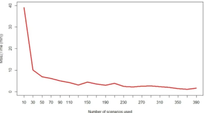
Figure 4 represents the evolution of this sizing error depending on the number of scenarios used in the simulation.
Figure 4: Evolution of the mean square sizing error with the number of scenarios considered in the simulation. Error is expressed in extra minutes of overshoot. Objective overshoot time (T): 19 minutes.
The error is very high when considering a few scenarios (under 50). There is up to 40 minutes of mean extra overshoot when considering few scenarios, increasing the probability to miss some high loaded scenarios. When
using more than 300 scenarios for the evaluation, the extra minutes of overshoot are evaluated to less than 2 minutes, representing less than 10% of the initial value.
CONCLUSION
Integration of decentralized means of production, e.g. photovoltaics and wind power, is impacting the network in several ways, on voltage, intensity etc. In this work we consider only the electricity demand peaks issues. When considering self-consumption, this local production can mitigate peaks of electricity demand, and thus permits the distribution system operator to connect a higher load for a same MV feeder. Indeed, depending on the renewable energy systems penetration rates, their integration on the network permits a small gain in grid sizing. For a same quality of supply, represented by the yearly mean overshoot time of the sizing power, we shown that RES permit to lower the sizing power by 4 % of the original value. This value, apparently low, would permit a DSO to connect new clients to a same MV feeder without reinforcement work, representing non negligible savings at a country level. The simulation has shown a reasonable accuracy (>90%) in terms of evaluation of the new sizing power when using more than 300 scenarios.
Two models have been developed to inject variability of the renewable production means, in order to be more realistic. Their impact has not been quantified, and might be elevated when the MV feeder is mostly producer of electricity (few or no consumers). It has to be noticed that the simulations have been led using a restricted amount of load and production curves, and the accuracy of the developed method would be increased by the inclusion of a bigger amount of scenarios.
REFERENCES
[1] IEA, 2014, Technology roadmap. Solar Photovoltaic Energy, 9-37.
[2] J. Dickert and P. Schegner, 2010, Residential load models for network planning purposes. In 2010 Modern
Electric Power Systems, 1–6.
[3] N. Kong, M. Bocquel, T. Barbier et al, 2017, “Long term forecast of local electrical demand and evaluation of future impacts on the electricity distribution network”, Proceedings CIRED conference.
[4] Vincent Lefieux, 2007, "Modèles semi-paramétriques appliqués à la prévision des séries temporelles. Cas de la consommation d’électricité", PhD thesis, Université Rennes 2.
[5] Thibaut Barbier, Robin Girard, François-Pascal Neirac, Nicolas Kong, Georges Kariniotakis, 2014, “A novel approach for electric load curve holistic modelling and simulation”. MedPower 2014, 221
[6] Espinar B., P. Blanc, L. Wald, B. Gschwind, L. Ménard, E. Wey, C. Thomas, L. Saboret, 2012. “HelioClim-3: a near-real time and long-term surface solar irradiance database”. COST-WIRE-ES1002: Workshop May
22nd-23rd 2012, Roskilde, Denmark.
[7] N.A. Engerer, F.P. Mills, 2014, “KPV: A clear-sky index for photovoltaics”, Solar Energy Volume 105, 679-693.
[8] Christelle Rigollier, Olivier Bauer, Lucien Wald, 2000, “On the clear sky model of the ESRA — European Solar Radiation Atlas — with respect to the heliosat method”, Solar Energy Volume 68 Issue 1, 33-48. [9] Rienecker, M.M., M.J. Suarez, R. Gelaro, R. Todling, J. Bacmeister, E. Liu, M.G. Bosilovich, S.D.
Schubert, L. Takacs, G.-K. Kim, S. Bloom, J. Chen, D. Collins, A. Conaty, A. da Silva, et al., 2011, “MERRA: NASA's Modern-Era Retrospective Analysis for Research and Applications”, J. Climate 24, 3624-3648.