HAL Id: hal-00838080
https://hal.inria.fr/hal-00838080v3
Submitted on 12 Sep 2013
HAL is a multi-disciplinary open access
archive for the deposit and dissemination of
sci-entific research documents, whether they are
pub-lished or not. The documents may come from
teaching and research institutions in France or
abroad, or from public or private research centers.
L’archive ouverte pluridisciplinaire HAL, est
destinée au dépôt et à la diffusion de documents
scientifiques de niveau recherche, publiés ou non,
émanant des établissements d’enseignement et de
recherche français ou étrangers, des laboratoires
publics ou privés.
A review of cosparse signal recovery methods applied to
sound source localization
Srđan Kitić, Nancy Bertin, Rémi Gribonval
To cite this version:
Srđan Kitić, Nancy Bertin, Rémi Gribonval. A review of cosparse signal recovery methods applied to
sound source localization. Le XXIVe colloque Gretsi, Sep 2013, Brest, France. �hal-00838080v3�
A review of cosparse signal recovery methods
applied to sound source localization
∗
Srdan Kiti´c1, Nancy Bertin2, R´emi Gribonval1
1Inria, Centre Inria Rennes - Bretagne Atlantique
Campus de Beaulieu, F-35042 Rennes Cedex, Rennes, France
2IRISA - CNRS UMR 6074
Campus de Beaulieu, F-35042 Rennes Cedex, Rennes, France srdjan.kitic@inria.fr, nancy.bertin@irisa.fr,
remi.gribonval@inria.fr
R´esum´e –L’objectif de cet article est de comparer plusieurs m´ethodes de l’´etat de l’art pour la reconstruction coparcimonieuse de signaux, dans le contexte de la localisation de sources sonores. Nous ´evaluons les performances de cinq algorithmes de reconstruction coparcimonieuse : l’algorithme de ”Greedy Analysis Structured Pursuit”, les minimisations `1 et `1,2 jointe, ainsi
que les algorithmes ”Structured Analysis Iterative Hard Thresholding” et ”Structured Analysis Hard Thresholding Pursuit”. Nous comparons ´egalement ces algorithmes `a l’approche de parcimonie `a la synth´ese, que nous r´esolvons par la minimisation jointe `1,2 correspondante. Nous illustrons nos r´esultats dans le cadre d’une application `a la localisation de sources sonores,
r´ealise sur des simulations de mesures de champs de pression acoustique.
Abstract –This work aims at comparing several state-of-the-art methods for cosparse signal recovery, in the context of sound source localization. We assess the performance of five cosparse recovery algorithms: Greedy Analysis Structured Pursuit, `1 and
joint `1,2 minimization, Structured Analysis Iterative Hard Thresholding and Structured Analysis Hard Thresholding Pursuit.
In addition, we evaluate the performance of these methods against the sparse synthesis paradigm, solved with corresponding joint `1,2 minimization method. For this evaluation, the chosen applicative showcase is sound source localization from simulated
measurements of the acoustic pressure field.
1
Introduction
Most real-life signals exhibit a so-called compressible struc-ture, which means that, if represented in a suitable do-main, most of the information they contain is inherently low-dimensional. This premise has been extensively used in inverse problems such as compressed sensing [1], where we seek to restore the original signal x ∈ Rn from a
set of undersampled and/or noisy linear measurements y= M x + ε ∈ Rmwith m < n.
This underdetermined problem can be regularized by a sparse prior, where we assume that the signal x may be represented as a linear combination of a few column vectors extracted from a dictionary Ψ ∈ Rn×d, n ≤ d,
weighted by some vector α ∈ Rd which has a small
num-ber k of non-zero coefficients compared to its dimension d. A significant amount of theoretical and empirical research has confirmed the usefulness of this, so-called sparse syn-thesis approach.
Beside sparse synthesis, an alternative approach termed
∗This work was supported in part by the European Research
Council, PLEASE project (ERC-StG-2011-277906).
sparse analysis or cosparse signal model [2] has emerged more recently. In this model, the product z = Ωx, where Ω ∈ Rp×n(p ≥ n), is assumed to be sparse. The matrix Ω is called the analysis operator, and may be, for example, the finite difference operator. Although equivalent when Ω is an invertible square matrix (Ω = Ψ−1), the two models differ as soon as p 6= d [3].
In order to emphasize the distinction, we say that the signal x is l-cosparse if l = p − kΩxk0< d. The cosparse
model has received less attention than the synthesis model so far. A foundation for cosparse signal modeling and counterparts of most common sparse synthesis methods can be found in [2, 4].
When the underlying sparse signal has a specific struc-ture (e.g., when non-zeros of α follow some particular pat-tern), it has been shown [5] that exploiting this structured sparsity contributes to better signal recovery. Joint spar-sity is one of these exploitable structure. In this case, the complete signal α can be described as a concatenation of sparse subsignals (α1, α2. . . αs), where each αi is of the
dimension d/s, and which all share the same support (i.e., the indices of nonzero elements are the same for all αi).
Similarly, we assume the signal x to be jointly cosparse, if the indices of zero-elements (called cosupport) in all zi
(subvectors of z = Ωx) are equal.
Our aim is to exploit the cosparse framework for solving a source localization problem, described in the following section.
2
Sound source localization in a 2D
acoustic pressure field
We wish to localize one or more sound sources, in a bounded two-dimensional space, from some linear measurements of the acoustic pressure field p(~r, t). At all non-boundary locations, the acoustic pressure will approximatively obey the acoustic wave equation:
∆p(~r, t) − 1 c2 ∂2p(~r, t) ∂t2 = ( 0, if no source at ~r f (~r, t), if source at ~r (1) Using the Finite Difference Method and second-order ap-proximations, the equation (1) can be discretized straight-forwardly. By taking into account the boundary and the initial conditions, we can then design an appropriate op-erator Ω ∈ Rd×d such that Ωp = 0 for all source-free
positions. Note that the operator Ω is very sparse, which is a convenient property in terms of computational cost.
Since the number of sources (s) is usually much smaller than the dimensionality of the discretized space, the sig-nal p is cosparse, and even joint-cosparse if we assume that sources are not moving. Hence, localizing the sources amounts to the noiseless cosparse recovery problem:
recover p from y = M p, s.t. kΩpk0 d,
and p is jointly cosparse. (2) We can also note that in this square case, a simple matrix inversion results in an equivalent synthesis model where the dictionary Ψ = Ω−1 are the Green’s functions. We will discuss the algorithmic disadvantages of usage of Green’s functions later in the text.
3
Algorithms and methods
In general, finding an exact solution for the cosparse regu-larization is known to be NP-hard [2].To circumvent this, different approximative methods have been proposed, out of which we consider the following in our study1:
`1 (analysis) minimization Standard `1 norm
mini-mization has been widely used for its property to produce sparse solutions and its convenient convexity [6]. In the context of the analysis model, it is used in the following manner: ˆp= arg minpkΩpk1, s.t. y = M p.
1The optimization algorithms are provided as a
public domain software (under GNU licence) at http://people.rennes.inria.fr/Srdan.Kitic/
Joint`1,2 (analysis) minimization The minimization
of the `1,2 norm [7] is equivalent to a minimization of `1
norm on groups gi,j of Ωp, which gather the variables
corresponding to each spatial index (i, j). The principle is to promote a small number of non-zero normed groups gi,j in space, while not imposing a restriction within a given group, in time. Spatial grouping of variables leads to the following formulation of the method:
ˆ
p= arg minpkZ(p)k1,2 s.t. y = M p
where Z(p) = devect2(Ωp). (3) GRASP As in the traditional sparse framework, cosparse recovery can also be addressed by greedy approaches. We retained here the use of GRASP - GReedy Analysis Struc-tured Pursuit [8], an algorithm which is partially based on Greedy Analysis Pursuit (GAP) [2]. It can be intuitively seen as an approximation of the mixed norm minimization described in previous paragraph (for the detailed descrip-tion, the reader may consult the referenced papers). Structured AIHT and AHTP Structured Analysis Iterative Hard Thresholding and Structured Analysis Hard Thresholding Pursuit are modified versions of Analysis It-erative Hard Thresholding and Analysis Hard Threshold-ing Pursuit algorithms presented in [2, 4]. We introduced a change in the joint cosupport selection step, very sim-ilar to the one used in GRASP, in order to make them structure-aware and allow a fairer comparison with the previous. Simultaneous HTP has been already developed for the synthesis model [9], but, to our best knowledge, this remained to be done for analysis IHT and HTP. Joint `1,2 (synthesis) minimization For comparison
purpose, we include in our benchmark an algorithm based on the synthesis paradigm for joint-sparse recovery, which minimizes the mixed `1,2 norm. As noted in section 1,
the synthesis and the analysis models should here produce the equivalent solutions ; however, the dictionary Ψ is not sparse, which vastly increases the computational cost in large-scale setting.
4
Experiments
The solution of a problem (2) depends on different param-eters. In order to be comprehensive, we have tested the recovery methods for various settings.
4.1
Simulation settings
The experiments were conducted in an artificial two di-mensional space, modeled as an uniform rectangular grid
2devect reshapes the input vector u into a matrix U such that
rows of U correspond to a spatial dimension, while columns repre-sent different time instances.
of size 20×20. The boundaries were modeled by Neumann or Dirichlet boundary conditions (d~n
d~r = 0 or p = const,
respectively). The time span of the experiments (the “ac-quisition” time) was either Ta1= 40 or Ta2= 100, whereas
the wave propagation speed was set to a constant value c = 0.2 (homogeneous medium).
For the physical settings described above, the appro-priate finite difference operators Ω were designed. The corresponding Green’s function dictionaries Ψ were gen-erated by taking the matrix inverse of the analysis oper-ators. As expected, the numerical density (the number of non-zeros) of these matrices is very different: the dic-tionaries contain approximately 20% of non-zero elements (depending on the boundary conditions) whereas for the operators this percentage is around 0.004%.
The first series of experiments compared the perfor-mance of recovery methods for the unit magnitude monochro-matic sources. Each source was assigned the random phase ϕ ∈ [0, 2π]. The second series of experiments investigated the localization of wideband sources. These were mod-eled as white Gaussian zero-mean processes of variance σ2
2= 0.04.
We present the results in the form of empirical prob-ability of accurate source localization, i.e. the number of correctly identified sources given the total number of sources in the experiment. The numbers of microphones m and sources s were varied relative to each other, and both were placed randomly in the spatial field. The x-axis in-dicates the ratio between the number of microphones and the total spatial dimension n, while the y-axis indicates the ratio between the number of sources and the number of microphones. The source locations were recovered after estimating the pressure signal p, by localizing s largest (in `2-norm sense) spatial positions of Ωp.
4.2
Results
The first six diagrams in Figure 1 depict the recovery of a lower frequency signal for the short acquisition time Ta1.
The presented diagrams are for the Neumann boundary condition, but we obtained almost identical results for the Dirichlet boundary as well. This trend continued through-out all the experiments, meaning that the performance was approximatively the same regardless the boundary condition applied. The results (a) and (b) clearly indicate the inferiority of SAIHT and SAHTP methods which, in addition, exhibited problems with the convergence. For concision purpose, these algorithms were omitted in the other experiments.
The diagrams (g), (h) and (i) show the significant im-provement gained by extending the acquisition time to Ta2. This is only feasible in the cosparse case, since the
dictionary of the appropriate size is extremely memory consuming (over 12Go in this setting). Hence, the results for the synthesis algorithm are not presented.
δ =m ρ = sm 0 0.1 0.2 0.3 0.1 0.2 0.3 0.4 0.5 0.6 0.7 0 0.2 0.4 0.6 0.8 1 (a) SAIHT Ta1= 40 δ =m ρ = sm 0 0.1 0.2 0.3 0.1 0.2 0.3 0.4 0.5 0.6 0.7 0 0.2 0.4 0.6 0.8 1 (b) SAHTP Ta1= 40 δ =m ρ = sm 0 0.1 0.2 0.3 0.1 0.2 0.3 0.4 0.5 0.6 0.7 0 0.2 0.4 0.6 0.8 1 (c) `1 analysis Ta1= 40 δ =m ρ = sm 0 0.1 0.2 0.3 0.1 0.2 0.3 0.4 0.5 0.6 0.7 0 0.2 0.4 0.6 0.8 1 (d) `1,2analysis Ta1= 40 δ =m ρ = sm 0 0.1 0.2 0.3 0.1 0.2 0.3 0.4 0.5 0.6 0.7 0 0.2 0.4 0.6 0.8 1 (e) `1,2 synthe-sis Ta1= 40 δ =m ρ = sm 0 0.1 0.2 0.3 0.1 0.2 0.3 0.4 0.5 0.6 0.7 0 0.2 0.4 0.6 0.8 1 (f) GRASP Ta1= 40 δ =m ρ = sm 0 0.1 0.2 0.3 0.1 0.2 0.3 0.4 0.5 0.6 0.7 0 0.2 0.4 0.6 0.8 1 (g) `1 analysis Ta2= 100 δ =m ρ = sm 0 0.1 0.2 0.3 0.1 0.2 0.3 0.4 0.5 0.6 0.7 0 0.2 0.4 0.6 0.8 1 (h) `1,2analysis Ta2= 100 Not computed δ =m ρ = sm 0 0.1 0.2 0.3 0.1 0.2 0.3 0.4 0.5 0.6 0.7 0 0.2 0.4 0.6 0.8 1 (i) GRASP Ta2= 100 δ =m ρ = sm 0 0.1 0.2 0.3 0.1 0.2 0.3 0.4 0.5 0.6 0.7 0 0.2 0.4 0.6 0.8 1 (j) `1 analysis Ta2= 100 δ =m ρ = sm 0 0.1 0.2 0.3 0.1 0.2 0.3 0.4 0.5 0.6 0.7 0 0.2 0.4 0.6 0.8 1 (k) `1,2analysis Ta2= 100 Not computed δ =m ρ = sm 0 0.1 0.2 0.3 0.1 0.2 0.3 0.4 0.5 0.6 0.7 0 0.2 0.4 0.6 0.8 1 (l) GRASP Ta2= 100 δ =m ρ = sm 0 0.1 0.2 0.3 0.1 0.2 0.3 0.4 0.5 0.6 0.7 0 0.2 0.4 0.6 0.8 1 (m) `1 analysis Ta1= 40 δ =m ρ = sm 0 0.1 0.2 0.3 0.1 0.2 0.3 0.4 0.5 0.6 0.7 0 0.2 0.4 0.6 0.8 1 (n) `1,2analysis Ta1= 40 δ =m ρ = sm 0 0.1 0.2 0.3 0.1 0.2 0.3 0.4 0.5 0.6 0.7 0 0.2 0.4 0.6 0.8 1 (o) `1,2 synthe-sis Ta1= 40 δ =m ρ = sm 0 0.1 0.2 0.3 0.1 0.2 0.3 0.4 0.5 0.6 0.7 0 0.2 0.4 0.6 0.8 1 (p) GRASP Ta1= 40 δ =m ρ = sm 0 0.1 0.2 0.3 0.1 0.2 0.3 0.4 0.5 0.6 0.7 0 0.2 0.4 0.6 0.8 1 (q) `1 analysis Ta2= 100 δ =m ρ = sm 0 0.1 0.2 0.3 0.1 0.2 0.3 0.4 0.5 0.6 0.7 0 0.2 0.4 0.6 0.8 1 (r) `1,2 analysis Ta2= 100 Not computed δ =m ρ = sm 0 0.1 0.2 0.3 0.1 0.2 0.3 0.4 0.5 0.6 0.7 0 0.2 0.4 0.6 0.8 1 (s) GRASP Ta2= 100
Figure 1: Probability of correct source localization for the low frequency signal ((a) - (i)), the high frequency signal ((j) - (l)) and the wideband signal ((m) - (s))
δ =m ρ = sm 0 0.1 0.2 0.3 0.1 0.2 0.3 0.4 0.5 0.6 0.7 (a) `1 analysis Ta1= 40 δ =m ρ = sm 0 0.1 0.2 0.3 0.1 0.2 0.3 0.4 0.5 0.6 0.7 (b) `1,2analysis Ta1= 40 δ =m ρ = sm 0 0.1 0.2 0.3 0.1 0.2 0.3 0.4 0.5 0.6 0.7 (c) `1,2 synthe-sis Ta1= 40 δ =m ρ = sm 0 0.1 0.2 0.3 0.1 0.2 0.3 0.4 0.5 0.6 0.7 (d) GRASP Ta1= 40
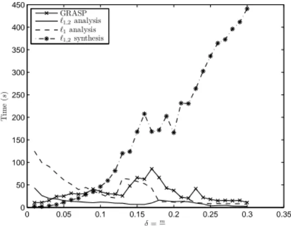
0 0.05 0.1 0.15 0.2 0.25 0.3 0.35 0 50 100 150 200 250 300 350 400 450 δ =m n T im e (s ) GRASP ℓ1,2analysis ℓ1analysis ℓ1,2synthesis
Figure 3: Average computation time
The following series ((j) - (l)) depicts the difference in lo-calization performance when the signal frequency is higher (f2). It has become evident that increasing the frequency
leads to a decrease in performance. The final series of experiments, (m) - (s), represents the algorithm’s perfor-mance in the case of a wideband signal.
Important fact is that the source localization perfor-mance is highly correlated with the success of a signal recovery (the underlying signal’s estimation error). This is illustrated in Figure 2 for the source localization exper-iments 1(c) - 1(f).
Figure 3 illustrates the average computation time ver-sus the relative number of samples for the four recovery methods. All cosparse methods are dramatically faster than the synthesis version of joint `1,2 minimization. We
observed that the more data becomes available, the slower the synthesis version gets, due to more linear operations needed per iteration. On the other hand, the analysis version gets faster, since the overall number of iterations becomes smaller.
5
Conclusion
We benchmarked several cosparse and one sparse recov-ery algorithms, for the particular case of synthetic wave signals.
Our experiments show that in the majority of cases, standard `1 norm minimization is the most robust
recov-ery method, whereas joint `1,2 minimization exhibits the
fastest convergence while being the second best in source localization. GRASP is a moderately fast algorithm, but its accuracy is considerably lower than the former two. The structure-aware AIHT and AHTP algorithms are the worst performing both in accuracy and processing time, which is related to the inexact cosparse projection step [10], based on the hard thresholding.
The synthesis and the analysis versions of joint `1,2
min-imization perform the same in terms of accuracy, but the cosparse version converges much faster due to the
spar-sity of analysis operator. Moreover, the cosparse methods allow for longer acquisition time, which improves the re-covery performance.
The signal frequency, the propagation speed and the discretization are closely related and impact the perfor-mance. The phenomenon is both physical and numerical, as a consequence of the discretization method’s limita-tions. Their interaction is out of the scope of this paper and remains to be investigated.
References
[1] D. Donoho, “Compressed sensing,” Information The-ory, IEEE Transactions on, vol. 52, no. 4, pp. 1289– 1306, 2006.
[2] S. Nam, M. E. Davies, M. Elad, and R. Gribonval, “The Cosparse Analysis Model and Algorithms,” Ap-plied and Computational Harmonic Analysis, vol. 34, no. 1, pp. 30–56, 2013. Preprint available on arXiv since 24 Jun 2011.
[3] M. Elad, P. Milanfar, and R. Rubinstein, “Analysis versus synthesis in signal priors,” tech. rep., 2005. [4] R. Giryes, S. Nam, M. Elad, R. Gribonval, and M. E.
Davies, “Greedy-Like Algorithms for the Cosparse Analysis Model,” arXiv preprint arXiv:1207.2456, 2013.
[5] M. Yuan, M. Yuan, Y. Lin, and Y. Lin, “Model selec-tion and estimaselec-tion in regression with grouped vari-ables,” Journal of the Royal Statistical Society, Series B, vol. 68, pp. 49–67, 2006.
[6] S. S. Chen, D. L. Donoho, Michael, and A. Saunders, “Atomic decomposition by basis pursuit,” SIAM Journal on Scientific Computing, vol. 20, pp. 33–61, 1998.
[7] R. Jenatton, J. Audibert, and F. Bach, “Structured variable selection with sparsity-inducing norms,” arXiv preprint arXiv:0904.3523, 2009.
[8] S. Nam and R. Gribonval, “Physics-driven structured cosparse modeling for source localization,” in Acous-tics, Speech and Signal Processing (ICASSP), 2012 IEEE International Conference on, pp. 5397–5400, IEEE, 2012.
[9] S. Foucart, “Recovering jointly sparse vectors via hard thresholding pursuit,” Proc. Sampling Theory and Applications (SampTA)],(May 2-6 2011), 2011. [10] A. M. Tillmann, R. Gribonval, and M. E. Pfetsch,
“Projection onto the k-cosparse set is np-hard,” CoRR, vol. abs/1303.5305, 2013.