Performance Analysis of CGS, a k-Coverage Algorithm Based on One-Hop Neighboring Knowledge

Abstract—We give numerically tractable, explicit integral ex- pressions for the distribution of the signal-to-interference-and- noise-ratio (SINR) experienced by a typical user in

[21] used a genetic algorithm to propose a solution heuristic to target coverage problem, that groups the sensor nodes of the network into subsets covering all targets, to form

 Majority (75%, n=12) selected an article where document type was in the Single Search display.. Majority of users

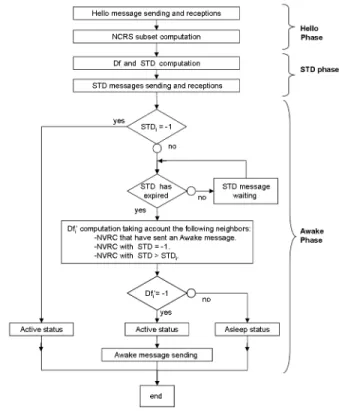
In this paper a new coordinated algorithm is proposed that is able to guarantee k-coverage in the network where it is physically possible and at the same time can provide

We report on a browser extension that seamlessly adds relevant microposts from the social networking sites Google + , Facebook, and Twitter in form of a panel to Knowledge

It is important to point out that both the fixed communication cost and the consumption rate depend on whether the particular sensor spends the period awake or asleep: sleeping

We show the behaviour of VFA-C, the combined version of the local variant of PSO and the VFA-D (PSO-S), by considering 1) the coverage, as the fraction of ZoI covered by sensors

At any time of the process, only k vertices can be kept in memory; if at some point the cur- rent solution already contains k vertices, any inclusion of any new vertex in the