HAL Id: hal-02906973
https://hal.archives-ouvertes.fr/hal-02906973
Submitted on 26 Jul 2020
HAL is a multi-disciplinary open access
archive for the deposit and dissemination of
sci-entific research documents, whether they are
pub-lished or not. The documents may come from
teaching and research institutions in France or
abroad, or from public or private research centers.
L’archive ouverte pluridisciplinaire HAL, est
destinée au dépôt et à la diffusion de documents
scientifiques de niveau recherche, publiés ou non,
émanant des établissements d’enseignement et de
recherche français ou étrangers, des laboratoires
publics ou privés.
DNNZip: Selective Layers Compression Technique in
Deep Neural Network Accelerators
Habiba Lahdhiri, Maurizio Palesi, Salvatore Monteleone, Davide Patti,
Giuseppe Ascia, Jordane Lorandel, Emmanuelle Bourdel, Vincenzo Catania
To cite this version:
Habiba Lahdhiri, Maurizio Palesi, Salvatore Monteleone, Davide Patti, Giuseppe Ascia, et al..
DNNZip: Selective Layers Compression Technique in Deep Neural Network Accelerators.
Euromi-cro Conference on Digital System Design DSD, Aug 2020, Portorož, Slovenia. �hal-02906973�
DNNZip: Selective Layers Compression Technique
in Deep Neural Network Accelerators
Habiba Lahdhiri
∗, Maurizio Palesi
†Salvatore Monteleone
∗, Davide Patti
†, Giuseppe Ascia
†, Jordane Lorandel
∗,
Emmanuelle Bourdel
∗, and Vincenzo Catania
†∗ ETIS UMR 8051, CY Cergy Paris University, ENSEA, CNRS, F-95000 Cergy, France.
{habiba.lahdhiri, salvatore.monteleone, jordane.lorandel, emmanuelle.bourdel}@ensea.fr
†Department of Electrical, Electronic, and Computer Engineering (DIEEI), University of Catania, I-95125 Catania, Italy. {maurizio.palesi, davide.patti, giuseppe.ascia, vincenzo.catania}@dieei.unict.it
Abstract—In Deep Neural Network (DNN) accelerators, the on-chip traffic and memory traffic accounts for a relevant fraction of the inference latency and energy consumption. A major component of such traffic is due to the moving of the DNN model parameters from the main memory to the memory interface and from the latter to the processing elements (PEs) of the accelerator. In this paper, we present DNNZip, a technique aimed at compressing the model parameters of a DNN, thus resulting in significant energy and performance improvement. DNNZip implements a lossy compression whose compression ratio is tuned based on the maximum tolerated error on the model parameters provided by the user. DNNZip is assessed on several convolutional NNs and the trade-off inference energy saving vs. inference latency reduction vs. network accuracy degradation is discussed. We found that up to 64% energy saving, and up to 67% latency reduction can be obtained with a limited impact on the accuracy of the network.
Index Terms—Approximate Deep Neural Networks, Deep Neural Network Accelerator, Weights Compression, Accu-racy/Latency/Energy Trade-off.
I. INTRODUCTION
Deep Neural Networks (DNNs) have been founding fertile ground in several application domains achieving dramatic accuracy improvements in many tasks as compared to tra-ditional handcrafted algorithms. While DNN-based methods often require significant computational, communication, and storage capabilities, there is a need to run them in real-time on resource constrained embedded and/or mobile systems. Thus, in the last few years, several dedicated hardware ac-celerators have been proposed for efficient inference compu-tation [1]–[3]. Their basic architecture consists of a matrix of processing elements (PEs) specialized to perform several multiply-accumulate operations per clock cycle interconnected by means of a customized network-on-chip (NoC) [4], [5].
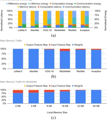
Current DNN models rely on millions or even billions of parameters, thus exacerbating the role played by the com-munication and memory sub-systems for moving such high data volume from the main memory into the accelerator and then to its many PEs. Thus, the performance and energy figures of a DNN accelerator are severely affected by the communication and memory sub-system [6], [7]. Fig. 1a shows the normalized latency and energy during the execution of an
inference for different network models1. As it can be observed,
the overall inference latency is due to the memory and on-chip communication latency. The overall inference energy is mainly due to memory (both on-chip local and off-chip main memory) and on-chip communication. There are three main types of traffic that determine the above latency and energy figures, as follows: 1) The traffic for fetching the input feature map and model parameters (i.e., weights) from the memory; 2) the on-chip traffic for dispatching the weights and the input feature map among the PEs of the accelerator; 3) the traffic for storing back the output feature map to the main memory in case of the local memory does not suffice. In particular, the fraction of traffic due to transfer weights accounts for a significant fraction of the overall traffic as shown in Fig. 1b. Further, in contrast to the traffic induced by the output feature maps that decreases as the accelerator’s local memory size increases, the weights induced traffic is not affected by the amount of local memory. Thus, as the local memory size increases, the memory traffic becomes more and more dominated by the weights-induced traffic as shown in Fig. 1c for the case of MobileNet.
Based on the above observations, reducing the memory footprint to store the model parameters would have a relevant positive impact on both the performance and energy metrics. Thus, in this paper, we present DNNZip, a new compression technique for reducing the memory footprint to store the weights and consequently the traffic induced for delivering them to PEs. DNNZip takes as inputs the DNN model and a user defined maximum tolerated error on the model parameters and returns the compressed model parameters to be stored into the memory. Each layer of the DNN is compressed with the appropriate compression level in such a way to do not exceed the aforementioned maximum error threshold. DNNZip implements a lossy compression, that is, the decompressed parameters differ from the original ones. Thus, the compressed DNN can be seen as an approximate version of the original DNN. The architecture of the decompression unit which is in-tegrated into each PE and which allows on-the-fly decompres-sion of the compressed parameters’ stream is also presented. 1Information about the reference architecture of the DNN accelerator and
Normalized Latency 0% Normalized Energy 25% 50% 75% 100% 0% 25% 50% 75% 100%
LeNet-5 AlexNet VGG-16 MobileNet ResNet Inception
MMemory energy LMemory energy Computation energy Communication energy Memory latency Computation latency Communication latency
Inference Latency and Energy
(a) 0% 25% 50% 75% 100%
LeNet-5 AlexNet VGG-16 MobileNet ResNet Inception
Output Feature Map Input Feature Map Weights
Main Memory Traffic
(b)
Local Memory Size 0% 25% 50% 75% 100% 2 KB 4 KB 8 KB 16 KB 32 KB 64 KB
Output Feature Map Input Feature Map Weights
Main Memory Traffic for MobileNet
(c)
Fig. 1. Breakdown of inference latency and energy (a) and memory traffic (b) for different network models. Memory traffic breakdown for MobileNet for different local memory sizes (c).
DNNZip is assessed on several DNN models covering a wide spectrum of complexities in terms of number of parameters and number/type of layers. The trade-off between performance improvement vs. energy saving vs. accuracy degradation for the execution of an inference is then discussed.
Although several techniques have been proposed in the context of model compression and acceleration for DNNs [8], we show how DNNZip is complementary to other compression techniques and can be applied on top of them for further improving performance and energy figures.
II. RELATEDWORK
Most of the compression methods proposed in literature focus on minimizing the model size. Methods based on param-eters pruning and sharing try to remove paramparam-eters that are not crucial to the model performance. Deep compression [9] first prunes the network by learning only the important connections then, it quantizes the weights to enforce weight sharing, and finally, Huffman coding is applied. The main drawback of this approach is that Huffman coding implies storing a large dictionary with a consequent area overhead making it unsuitable for lightweight and energy-efficient implementa-tions. Other methods modify the network structure in order to compress weights. For instance, a unified end-to-end learning framework for learning compressible representations, jointly optimizing the model parameters, the quantization levels, and the entropy of the resulting symbol stream to compress the
network model is presented in [10]. A method to compress intermediate feature maps to decrease memory storage and bandwidth requirements during inference is presented in [11]. It is based on converting fixed-point activations into vectors over the smallest GF(2) finite field followed by nonlinear dimensionality reduction layers embedded into a DNN. The main drawback of compression representation learning based approaches is that they alter the DNN model and then require a retraining phase. EBPC [6] is a hardware-friendly and lossless compression scheme for the feature maps present within CNNs. However it is limited on the compression of the feature maps although the model parameters/weights are responsible for a major fraction of the overall memory/communication traffic (see Fig. 1b). Several compression techniques are based on reducing the number of bits required to represent weights with a consequent reduction of the memory footprint for storing the network parameters [12]. A direct consequence of quantization is the possibility of using arithmetic hardware modules working on lower data width, with a consequent improvement in silicon area and energy consumption. Extrem-izing quantization techniques, binarization allows to represent weights with just a single bit [13], [14]. Interested reader can refer to [8] for a survey of model compression and acceleration for DNNs.
As we will see in the rest of the paper, DNNZip does not compete with the aforementioned model compression techniques but it is rather orthogonal to them and it can be applied on top of them for further increasing their compression effectiveness.
III. DNNZIP
A. Compression Technique
To compress the model parameters one might think to apply one of the many available general data compression techniques. There are, however, two main issues that make such choice inappropriate/unfeasible in the considered context. First, conventional compression techniques rely on exposing redundant patterns in the data set by encoding them with a reduced number of bits as respect to that used for encoding less frequent patterns. Unfortunately, the entropy of the DNN parameters is close to that of random data making thus ineffective the use of conventional compression techniques. Second, conventional compression techniques are usually im-plemented in software and the decompression algorithm is often too complex to be implemented in hardware. In contrast, in our context, we are interested in extremely simple hardware decompression logic able to perform on-the-fly decompression of the compressed model parameters right before they are delivered to the PEs.
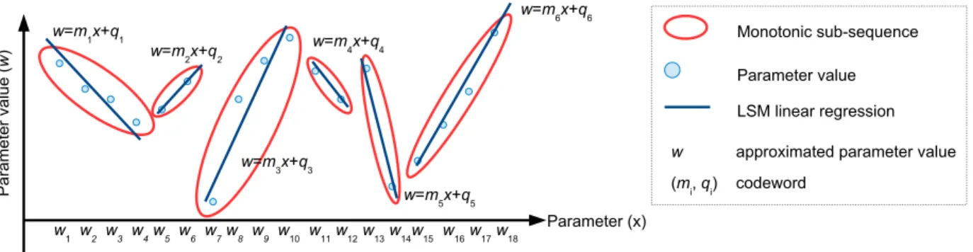
The compression technique implemented in DNNZip com-presses each layer as follows. Firstly, the parameters of the layer are sequentially parsed to extract monotonic sub-sequences of parameters. Then, for each sub-sequence, a linear regression based on the least squares criterion is used to determine the two coefficients of the line that approximates the values in the sub-sequence. The two coefficients, for each
sub-sequence, are the codewords which form the compressed model parameters to be stored into memory. To further in-crease the compression ratio, the strict monotonic definition is relaxed with a weak monotonic definition in which a tolerance factor δ is introduced as follows. A sub-sequence {w1, w2, . . . , wn} is monotonic decreasing in the weak sense
with tolerance threshold δ if:
wi > wi+1∨ |wi− wi+1| ≤ δ ∀ i = 1, 2, . . . , n − 1. (1)
Fig. 2 shows a graphic description of the compression tech-nique implemented by DNNZip. Please note that, in the rest of the paper we refer to δ as fraction of the amplitude of the set of the considered parameters. For instance, δ = 0.1 means 0.1 × (max P − min P ) where P is the considered set of parameters to be compressed.
B. Decompression Unit
Compressed parameters are stored into the main memory and are decompressed by a decompression unit embedded into each PE of the accelerator. The decompression unit generates the sub-sequence of approximated parameters [see Fig. 2(a)] starting from the codeword (m, q). As the approximated parameters are the points of the line with (m, q), they can be generated as ˜wi= ˜wi−1+ m for i = 2, . . . , N , where ˜w1= q
and N is the length of the sub-sequence. The organization of the decompression unit is shown in Fig. 3. As it can be observed the datapath requires a single adder and a register for storing the current generated approximate parameter ˜wi,
whereas the control unit can be simply implemented by means of a two states finite state machine.
The decompression unit has been synthesized at gate level with Synopsys Design Compiler and implemented with Synop-sys IC Compiler. The values of the implemented macro take also into account the overhead due to clock tree and scan flip flops for DFT. Finally the sign-off has been made with Synopsys Prime Time after that parasitics have been extracted by means of Synopsys Star RC. For the entire implementation flow a 16 nm technology standard cells library has been used. The decompression unit has been integrated into the PE [Fig. 3(b)] which is similar to that used in Simba platform [5] and features a 32 KB of local memory to temporary store weights, and a bank of parallel vector multiply-and-add units each able to perform 8:1 dot-product. The decompression unit occupies an area of 1008 µm2, has a critical path of 0.49 ns,
and a power consumption of 58 µW that is less than 1%, both in terms of area and power, than that of the PE.
C. Compression Flow
The DNN compression flow is shown in Fig. 4. First a sensitivity analysis is carried out to determine the most sensitive layers with respect to the approximation of their parameters (cf. Sec. III-C1). The sensitivity level (SL) of each layer along with the size of the set of parameters in each layer are used to compute a score for each layer (cf. Sec. III-C2). The scores along with a user defined maximum tolerated error on the model parameters (NMSEmax) are used
to determine the order in which layers are compressed to derive the approximate (i.e., compressed) networks and the appropriate δ value for each layer (cf. Sec. III-C3). The output of the flow is a set of compressed DNNs differing each other by the number of compressed layers. The three main steps of the compression flow are described in more detail in the following.
1) Sensitivity Analysis: Let Acc be the top 1 accuracy of the original DNN for test data set DS. Let P (Li) be the set
of parameters of layer Li. A portion pp of the parameters
is perturbed with a perturbation intensity pi. Perturbing a parameter means randomly adding/subtracting a fraction pi of its value. The perturbed DNN is tested and its top 1 accuracy is computed for DS. This process is repeated a number of times until reaching the 95% confidence for ±1% of the mean of the accuracies. Let Acci be the mean of the top 1 accuracies
of the perturbated DNNs. The sensitivity level of layer Li is
then computed as SL(Li) = (Acc − Acci)/Acc.
2) Scores Computation: The sensitivity level and the size of the layer (i.e., the number or parameters of the layer) are used to compute the score of the layer. Specifically, high scores are assigned to large and low sensitive layers. This is because it is more convenient to compress those layers accounting for a higher fraction of the total parameters and, at the same time, are less sensitive to the approximation of their parameters. Based on this, the score S(Li) assigned to
layer Li is directly proportional to its number of parameters
and inversely proportional to its sensitivity level, that is, S(Li) = |P (Li)|/SL(Li).
3) Layers Compression: The last step of the compression
flow is the actual layers’ compression. First, layers are sorted based on their score. Let {s1, s2, . . . , sN L} be such that
S(Ls1) > S(Ls2) > . . . > S(LsN L) where N L is the number
of layers. Then, we consider N L different compressed DNNs, namely, xDN N1, xDN N2, . . . , xDN NN L where xDN Ni
is the compressed DNN in which layers Ls1, . . . , Lsi are
compressed, whereas the remaining layers Lsi+1, . . . , LsN L
are left uncompressed.
The generic layer Li is compressed with an appropriate
δ value which is selected based on the maximum tolerated error on the weights provided by the user. Such error is expressed as the normalized mean squared error (NMSE) as respect to the amplitude of the parameters of Li. That is,
N M SE = M SE/[max P (Li)−min P (Li)]. The appropriate
δ value is the maximum δ that can be used to compress the layer without exceeding the maximum NMSE provided by the user. The algorithm for computing the maximum delta value is shown in Alg. 1. The algorithm takes in input the layer to be compressed and the maximum tolerated NMSE and returns the compressed layer. Starting from the highest δ value of 1, it compresses the layer with the current δ value (line 4). Then, the NMSE between the original parameters and the approximated parameters (i.e., the reconstructed parameters from the compressed ones) is computed (line 5). If the NMSE is greater than the maximum tolerated NMSE threshold, it means that the current δ value is too high. Then, δ is reduced
P ar am et er v al ue ( w ) Parameter (x) w1 w2 w3 w4 w5 w6 w7 w8 w9 w10 w11 w12 w13 w14w15 w16 w17 w18 w=m1x+q1 w=m2x+q2 w=m3x+q3 w=m4x+q4 w=m5x+q5 w=m6x+q6 Monotonic sub-sequence Parameter value LSM linear regression
w approximated parameter value
(mi, qi) codeword
Fig. 2. Formation of the monotonic sub-sequence and their approximation by means of linear regression based on the least squares criterion.
m, q, N + wi m q Ctrl N mq rst Init/ 11 Run/00 cnt := 0 cnt := cnt + 1 cnt = N N mq rst Ctrl true (a) (b)
Fig. 3. Datapath and control logic of the decompression unit (a). Block diagram of the processing element (b).
NMSE
max
DNN SensitivityAnalysis ComputationScores Sensitivity Levels (SL) Layers Compression Scores (SC) Compressed Parameters Parameters set size
DNN parameters
Fig. 4. DNN compression flow.
by a certain amount (0.1% in the experiments in the next section). Otherwise, the current compressed layer is saved and the loop is terminated. The loop is also terminated if δ becomes negative. It means that, the layer cannot be
compressed without violating the NMSEmax constraint. In
such a case, the returned xLayer is NULL and the layer is not compressed.
Algorithm 1: Compute the maximum δ value to com-press a layer without exceeding the maximum NMSE threshold.
Data: Layer, NMSEmax
Result: xLayer
1 xLayer ← NULL;
2 δ ← 1;
3 repeat
4 xLayer0 ← Compress(Layer, δ);
5 NMSE ← ComputeNMSE(Layer, xLayer0);
6 if NMSE > NMSEmax then
7 Decrease δ; 8 else 9 xLayer ← xLayer0; 10 break; 11 end 12 until δ < 0; IV. EXPERIMENTS
In this section, we assess DNNZip on different CNN models used in image classification problems. However, other deep learning models such as Recurrent Neural Networks (RNNs) for speech/natural language applications can also be explored
in future work. We consider six representative CNN models, namely, LeNet-5, AlexNet, VGG-16, MobileNet, Inception-v3, and ResNet-50 which cover a wide spectrum in terms of complexity both in the number and type of layers and number of parameters.
A. Compression Analysis
We start by assessing the compression ratio and the corre-sponding accuracy loss when DNNZip is applied on different CNNs. First, we show in detail the steps of the compression flow described in Sec. III-C. Then, we summarize the results obtained for the remaining CNNs.
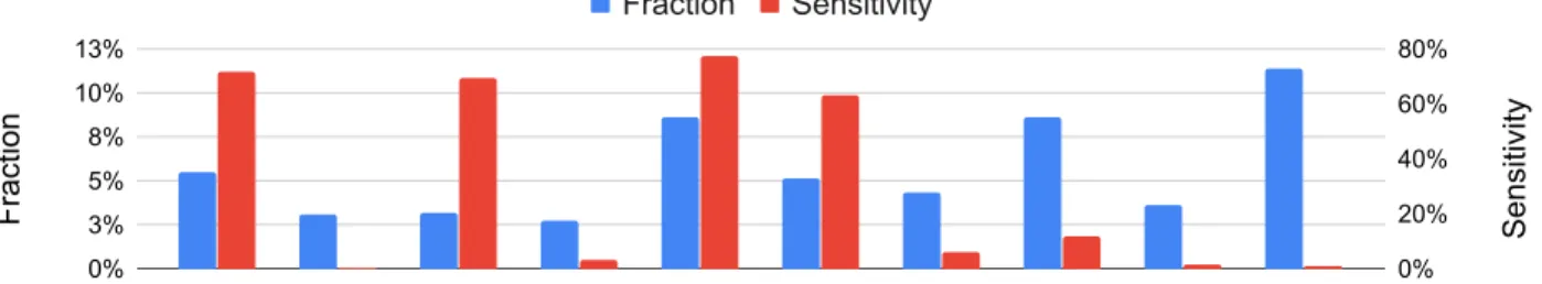
1) Compression Flow applied to Inception-v3: We consider Inception-v3 as reference CNN to show in detail the different steps of the compression flow. The first phase is the sensitivity analysis. In the experiments we consider a perturbation portion of 10% and a perturbation intensity of 5%. We select the 10 largest layers (in terms of number of parameters) out of 48 layers of Inception-v3. Their fraction as respect to the total number of parameters is shown in Fig. 5. The selected layers account for the 56% of the total model parameters. The figure also shows the sensitivity level of each considered layer. The less sensitive layer is predictions (with a sensitivity level less than 1%) which is also the largest one (it accounts for approx 11% of the total parameters). The size of a layer (i.e., its number of parameters) divided by its sensitivity level is used to compute the score of the layer, Fig. 6. The score assigned to a layer provides the suitability to compress that particular layer. In fact, more suitable layers to be compressed are large layers (that account for a large fraction of the total parameters) and low sensitive layers (that less impact the network accuracy when their parameters are approximated, i.e., compressed).
We generate 10 compressed (i.e., approximated) versions of Inception-v3, namely, Inception-x1, Inception-x2, . . ., Inception-x10 where Inception-xn is the approximated net-work in which the n layers with the highest scores are compressed. Each layer is compressed with a specific δ value computed as described in Alg. 1. In the experiments, we use
a NMSEmax of 0.05%. We found a high degradation of the
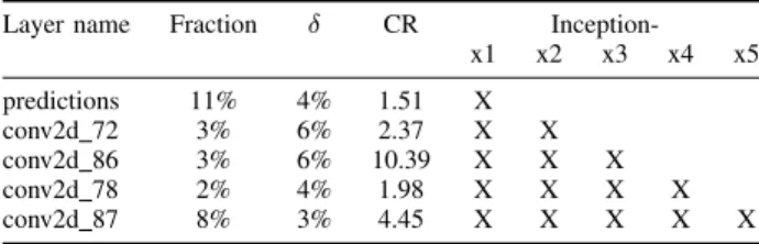
network accuracy when compressing more than 5 layers thus the analysis is limited to the first five compressed versions. Tab. I reports the δ value used for compressing the specific layer, along with its compression ratio (CR) and the indication of the layers compressed in each considered approximated version. Fig. 7 shows the memory footprint reduction and the top 5 accuracy of Inception and its five compressed versions. By compressing only one layer, which is the case of Inception-x1, with a δ of 4%, the reduction of the memory footprint is 9% and there is no remarkable accuracy degradation. We notice that, the percentage of the memory footprint saving increases with the number of compressed layers until reaching 52% without degradation of the accuracy. The limitation on 5 compressed layers is due to the fact that the other layers do not meet the constraint defined by the considered NMSEmax.
TABLE I
COMPRESSION RATIO ANDδVALUE FOR EACH COMPRESSED LAYER.
Layer name Fraction δ CR
Inception-x1 x2 x3 x4 x5 predictions 11% 4% 1.51 X conv2d 72 3% 6% 2.37 X X conv2d 86 3% 6% 10.39 X X X conv2d 78 2% 4% 1.98 X X X X conv2d 87 8% 3% 4.45 X X X X X
2) Summary of the Compression Analysis: DNNZip is
ap-plied to the rest of the CNNs and the results are summarized in Tab. II. The experiments have been carried out by considering
a NMSEmax of 0.05%. For each CNN, the table reports
the names of the compressed layers, the δ value computed with Alg. 1, the compression ratio (CR), the weighted CR, the memory footprint reduction, and the top 5 accuracy. The weighted CR is the CR weighted by the size of the layer as respect to the total number of parameters. The memory footprint reduction is the reduction in terms of bytes for storing the parameters of the CNN passing from the original model to the compressed model. The first row in each group reports the results for the original CNN whereas the subsequent rows reports the results for the approximated (i.e., compressed) CNNs. These latter are identified with the same name of the original CNN with the suffix -xn, where n is the number of compressed layers. Please note that, the compressed layers in *-xi approximated CNN are the same of that in *-x(i − 1) plus the one reported in its row. For instance, in AlexNet-x3 the compressed layers are dense1, dense2, and conv2d4. The table reports the results up to three compressed layers as, for most of the considered CNNs, the network accuracy rapidly decreases when more than three layers are compressed. As it can be observed, except for MobileNet, the memory footprint reduction is, on average, over 50% with an accuracy loss that is, in several cases, less than 5%.
The memory footprint reduction has a positive impact on both latency and energy metrics, and is assessed in the next subsection.
B. Latency and Energy Analysis
The previous results show how DNNZip provides a high compression ratio which then leads to a significant reduction in memory footprint without a major accuracy degradation. In this section, we focus on its impact on the inference latency and the inference energy. As baseline DNN accelerator we consider a Simba chiplet [5] which contains an array of PEs interconnected by means of a 4 × 4 mesh-based NoC. Each PE includes a 32 KB weight buffer and 8 parallel vector MAC units each of one able to perform 8:1 dot-product operations. The PE is augmented with the decompression unit described in Sec. III-B. The RTL models of the PE and router have been synthesized with Synopsis Design Compiler, implemented with Synopsys IC Compiler, and mapped on a 16 nm technology standard cells library. The links have been modelled with HSPICE and the parasitics extraction from
Fraction Sensitivity 0% 3% 5% 8% 10% 13% 0% 20% 40% 60% 80%
conv2d_27 conv2d_72 conv2d_81 conv2d_78 conv2d_82 conv2d_90 conv2d_87 conv2d_91 conv2d_86 predictions
Fraction Sensitivity
Fig. 5. Fraction of parameters and sensitivity level for each of the considered layers.
0,00 5,00 10,00 15,00 20,00
conv2d_27 conv2d_72 conv2d_81 conv2d_78 conv2d_82 conv2d_90 conv2d_87 conv2d_91 conv2d_86 predictions
Score
Fig. 6. Scores assigned to each of the considered layers.
Memory footprint 0% 20% 40% 60% 0,00 0,25 0,50 0,75 1,00
Inception Inception-x1 Inception-x2 Inception-x3 Inception-x4 Inception-x5
Mem footprint saving Top 5 Accuracy
Fig. 7. Memory footprint reduction and the top 5 accuracy of Inception and its five compressed versions.
layout has been made using Cadence Virtuoso. The power figures collected by the circuit level analysis have been used to back-annotate the cycle-accurate NoC simulator [15], [16]. For memory, both local and main memory, we used CACTI [17] to estimate the energy consumption (both leakage and dynamic) and timing information.
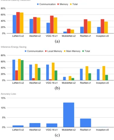
Fig. 8 shows the inference latency, energy, and accuracy reduction when DNNZip is applied on the CNN models analyzed in the previous subsection. For each CNN model we selected a specific compressed instance among those reported in Tab. II. Specifically, for each CNN, we selected the compressed instance for which the memory footprint saving is remarkably higher then the consequent accuracy loss. Fig. 8a shows the percentage inference latency reduction of communication and memory. The communication latency is the component due to the NoC for dispatching the weights and the feature maps among the PEs. The memory latency is the component due to fetch/store feature maps and weights from/to the main memory. We do not report the computation latency (i.e., the component due to the PEs for performing
dot-products operations, pooling, and activation computations) as it is unaffected by the application of DNNZip. In fact, the number of operations per inference does not change as computations are carried out on decompressed parameters. The graph reports also the total latency saving in which all the three components of the latency are taken into account. On average, 43% of total inference latency reduction is observed with 31% communication latency reduction and 47% main memory latency reduction. As expected, the highest latency reductions are observed for LeNet-5, AlexNet, and VGG-16 in which the compressed layers account for a significant fraction of the total parameters as compared to the other CNNs. MobileNet exhibits the lowest inference latency reduction. This is due to the fact that, its layers are almost all the same size (i.e., the same number of parameters) and the compression of few of them (two in the considered compressed instance) results in limited traffic reduction. Thus, a limitation of DNNZip is that of not being very effective in the case of network models with a low variance in layers size. Inference energy saving results are shown in Fig. 8b in which we report the two components
TABLE II
MEMORY FOOTPRINT REDUCTION AND ACCURACY LOSS WHENDNNZIP IS APPLIED ON DIFFERENTCNNS.
Network Compressed Fraction δ CR Weighted Mem fp Top-5
Model layer CR reduction Accuracy
LeNet-5 — — — — — — 0.9995 LeNet-5-x1 dense 2 16% 18% 2.22 1.20 16% 0.9994 LeNet-5-x2 dense 1 78% 20% 4.01 3.55 71% 0.9901 LeNet-5-x3 conv2d 2 3% 20% 3.16 3.64 72% 0.8720 AlexNet — — — — — — 0.9794 AlexNet-x1 dense 1 4% 13% 2.42 1.06 6% 0.9794 AlexNet-x2 dense 2 70% 13% 3.53 2.85 65% 0.9588 AlexNet-x3 conv2d 4 4% 13% 3.03 2.94 66% 0.9205 VGG-16 — — — — — — 0.8559 VGG-16-x1 fc1 74% 8% 5.28 4.24 76% 0.8395 VGG-16-x2 predictions 3% 3% 1.38 4.26 76% 0.8355 VGG-16-x3 fc2 12% 8% 1.66 4.34 78% 0.8195 MobileNet — — — — — — 0.9064 MobileNet-x1 conv pw 13 24% 2% 1.55 1.15 13% 0.7916
MobileNet-x2 conv preds 24% 1% 1.29 1.22 19% 0.7842
MobileNet-x3 conv pw 7 6% 2% 1.59 1.26 21% 0.7018 Inception — — — — — — 0.9720 Inception-x1 predictions 11% 4% 1.51 1.10 9% 0.9720 Inception-x2 conv2d 72 3% 6% 2.37 1.17 15% 0.9720 Inception-x3 conv2d 86 3% 6% 10.39 1.78 44% 0.9720 ResNet — — — — — — 0.9440
ResNet-x1 res5c branch2b 9% 8% 8.35 2.05 51% 0.9020
ResNet-x2 fc1000 8% 3% 2.37 2.22 55% 0.8730
ResNet-x3 res5c branch2c 4% 5% 3.77 2.40 58% 0.8570
considered in the latency analysis with the inclusion of the energy component due to the local memory. On average, 30% total inference energy saving is observed with 42%, 7%, and 47%, communication, local memory, and main memory energy reduction, respectively. The low energy saving for MobileNet is due to the same causes outlined above for the inference latency. Finally, Fig. 8c shows the loss of accuracy due to the application of DNNZip. With exception of MobileNet, less than 5% in accuracy loss is observed and for most of them (LeNet-5, AlexNet, VGG-16, and Inception), the accuracy loss is less than 2%.
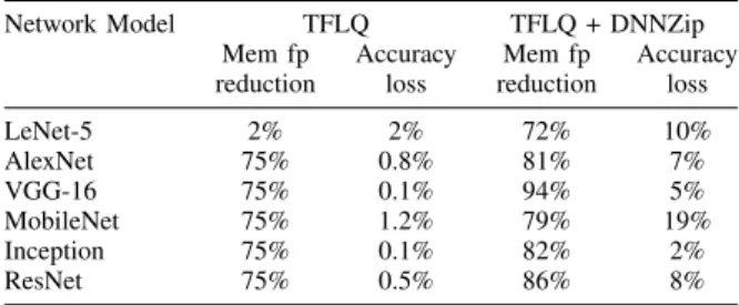
C. DNNZip on top of TensorFlow Lite Quantization
DNNZip can be used to further increase the compression efficiency of other model compression techniques. Several compression techniques are based on reducing the number of bits required to represent the model parameters with a consequent reduction of the memory footprint and the possi-bility of using arithmetic hardware modules working on lower data width, with a consequent improvement in silicon area and energy consumption [12]. We apply DNNZip on top of TensorFlow Lite quantization (TFLQ), introduced by Google as part of the DeepMind project [18]. Tab. III reports the memory footprint reduction and the accuracy loss for the two cases. As it can be observed, TFLQ provides, in almost all the cases, a memory footprint saving of 75% as the parameters are down scaled from 32 bits to 8 bits. Only for LeNet-5, the saving is low as only 2 out of 5 of its layers are compressed. The accuracy loss is negligible. When DNNZip
0% 20% 40% 60% 80%
LeNet-5-x2 AlexNet-x2 VGG-16-x1 MobileNet-x2 ResNet-x1 Inception-x5
Communication Memory Total
Inference Latency Reduction
(a) 0% 20% 40% 60% 80%
LeNet-5-x2 AlexNet-x2 VGG-16-x1 MobileNet-x2 ResNet-x1 Inception-x5
Communication Local Memory Main Memory Total
Inference Energy Saving
(b)
0% 5% 10% 15%
LeNet-5-x2 AlexNet-x2 VGG-16-x1 MobileNet-x2 ResNet-x1 Inception-x5
Accuracy Loss
(c)
Fig. 8. Latency reduction, energy saving, and accuracy loss when DNNZip is applied on different CNNs.
TABLE III
MEMORY FOOTPRINT REDUCTION AND ACCURACY LOSS WHENDNNZIP IS APPLIED ON TOP OFTENSORFLOWLITE QUANTIZATION(TFLQ).
Network Model TFLQ TFLQ + DNNZip
Mem fp Accuracy Mem fp Accuracy
reduction loss reduction loss
LeNet-5 2% 2% 72% 10% AlexNet 75% 0.8% 81% 7% VGG-16 75% 0.1% 94% 5% MobileNet 75% 1.2% 79% 19% Inception 75% 0.1% 82% 2% ResNet 75% 0.5% 86% 8%
is applied on the TFLQ compressed network, an additional memory footprint saving is observed with an accuracy loss that is less than 10% in most of the cases.
V. CONCLUSIONS
In this paper, we presented DNNZip, a compression tech-nique aimed at reducing the memory footprint for storing the model parameters of DNNs with consequent improvements in both inference latency and energy consumption. DNNZip selectively compresses the layers of a DNN with the most appropriate compression level in such a way to do not exceed a user defined error threshold defined in terms of the maxi-mum tolerated error on the model parameters. The hardware decompression unit integrated into the PEs of a reference DNN accelerator has been also presented. DNNZip has been assessed on several CNNs and the trade-off inference energy consumption vs. inference latency vs. accuracy loss has been discussed. We found that up to 64% energy saving, and up to 67% latency reduction can be obtained with a limited impact on the accuracy of the network.
ACKNOWLEDGEMENTS
This work has been supported by the following institu-tions/grants: (i) the Italian Ministry of Economic Development (MISE) within the research program “UE-PON Imprese e Competitivit`a 2014-2020 Contratto di sviluppo M9 (CDS 000448)” - CUP: C32F18000100008; (ii) the Institute of Advanced Studies of the CY Cergy Paris Universit´e (formerly Universit´e de Cergy-Pontoise) under the Paris Seine Initiative for Excellence (“Investissements d’Avenir” ANR-16-IDEX-0008); (iii) the DIEEI at University of Catania within the research program “Piano per la Ricerca 2016/2018”; (iv) the HiPEAC5 Network, financed by the European Union’s Horizon2020 research and innovation programme, under grant agreement number 779656.
REFERENCES
[1] B. Moons, R. Uytterhoeven, W. Dehaene, and M. Verhelst, “14.5 en-vision: A 0.26-to-10tops/w subword-parallel dynamic-voltage-accuracy-frequency-scalable convolutional neural network processor in 28nm fdsoi,” in IEEE International Solid-State Circuits Conference, Feb 2017, pp. 246–247.
[2] S. Yin, P. Ouyang, S. Tang, F. Tu, X. Li, L. Liu, and S. Wei, “A 1.06-to-5.09 tops/w reconfigurable hybrid-neural-network processor for deep learning applications,” in Symposium on VLSI Circuits, June 2017, pp. C26–C27.
[3] J. Lee, C. Kim, S. Kang, D. Shin, S. Kim, and H.-J. Yoo, “Unpu: A 50.6tops/w unified deep neural network accelerator with 1b-to-16b fully-variable weight bit-precision,” in 2018 IEEE International Solid - State Circuits Conference, Feb 2018, pp. 218–220.
[4] Y.-H. Chen, T.-J. Yang, J. Emer, and V. Sze, “Eyeriss v2: A flexible accelerator for emerging deep neural networks on mobile devices,” IEEE Journal on Emerging and Selected Topics in Circuits and Systems, vol. 9, no. 2, pp. 292–308, June 2019.
[5] Y. S. Shao, J. Clemons, R. Venkatesan, B. Zimmer, M. Fojtik, N. Jiang, B. Keller, A. Klinefelter, N. Pinckney, P. Raina, S. G. Tell, Y. Zhang, W. J. Dally, J. Emer, C. T. Gray, B. Khailany, and S. W. Keckler, “Simba: Scaling deep-learning inference with multi-chip-module-based architecture,” in IEEE/ACM International Symposium on Microarchitec-ture, 2019, pp. 14–27.
[6] L. Cavigelli, G. Rutishauser, and L. Benini, “Ebpc: Extended bit-plane compression for deep neural network inference and training accelerators,” IEEE Journal on Emerging and Selected Topics in Circuits and Systems, 2019.
[7] V. Catania, A. Mineo, S. Monteleone, M. Palesi, and D. Patti, “Im-proving the energy efficiency of wireless network on chip architectures through online selective buffers and receivers shutdown,” in 2016 13th IEEE Annual Consumer Communications Networking Conference (CCNC), 2016, pp. 668–673.
[8] Y. Cheng, D. Wang, P. Zhou, and T. Zhang, “A survey of model compression and acceleration for deep neural networks,” 2017. [9] S. Han, H. Mao, and W. Dally, “Deep compression: Compressing deep
neural networks with pruning, trained quantization and huffman coding,” in International Conference on Learning Representations, 10 2016. [10] E. Agustsson, F. M. E. Zurich, M. Tschannen, L. Cavigelli, R. Timofte,
and L. B. L. V. Gool, “Soft-to-hard vector quantization for end-to-end learning compressible representations,” in International Conference on Neural Information Processing Systems, 2017, pp. 1141–1151. [11] D. A. Gudovskiy, A. Hodgkinson, and L. Rigazio, “DNN feature map
compression using learned representation over GF(2),” in European Conference on Computer Vision, Sep 2018.
[12] Y. Choi, M. El-Khamy, and J. Lee, “Towards the limit of network quantization,” CoRR, vol. abs/1612.01543, 2016.
[13] M. Rastegari, V. Ordonez, J. Redmon, and A. Farhadi, “Xnor-net: Imagenet classification using binary convolutional neural networks,” in ECCV, 2016.
[14] M. Courbariaux and Y. Bengio, “Binarynet: Training deep neural net-works with weights and activations constrained to +1 or -1,” CoRR, vol. abs/1602.02830, 2016.
[15] V. Catania, A. Mineo, S. Monteleone, M. Palesi, and D. Patti, “Cycle-accurate network on chip simulation with noxim,” ACM Transactions on Modeling and Computer Simulation, vol. 27, no. 1, pp. 4:1–4:25, Nov. 2016.
[16] ——, “Energy efficient transceiver in wireless network on chip architec-tures,” in 2016 Design, Automation Test in Europe Conference Exhibition (DATE). Dresden, Germany: IEEE Computer Society, March 2016, pp. 1321–1326.
[17] R. Balasubramonian, A. B. Kahng, N. Muralimanohar, A. Shafiee, and V. Srinivas, “Cacti 7: New tools for interconnect exploration in innovative off-chip memories,” ACM Transactions on Architecture and Code Optimization (TACO), vol. 14, no. 2, pp. 1–25, 2017.
[18] Google DeepMind, “Tensorflow lite.” [Online]. Available: https://www.tensorflow.org/lite/