HAL Id: hal-00904743
https://hal.inria.fr/hal-00904743
Submitted on 18 Nov 2013
HAL is a multi-disciplinary open access
archive for the deposit and dissemination of
sci-entific research documents, whether they are
pub-lished or not. The documents may come from
L’archive ouverte pluridisciplinaire HAL, est
destinée au dépôt et à la diffusion de documents
scientifiques de niveau recherche, publiés ou non,
émanant des établissements d’enseignement et de
Processors
Arthur Perais, André Seznec
To cite this version:
Arthur Perais, André Seznec. Practical Data Value Speculation for Future High-end Processors.
[Research Report] RR-8395, INRIA. 2013, pp.21. �hal-00904743�
0249-6399 ISRN INRIA/RR--8395--FR+ENG
RESEARCH
REPORT
N° 8395
November 2013Practical Data Value
Speculation for Future
High-end Processors
RESEARCH CENTRE
RENNES – BRETAGNE ATLANTIQUE
High-end Processors
Arthur Perais, André Seznec
Project-Teams ALF
Research Report n° 8395 — November 2013 — 21 pages
Abstract: Dedicating more silicon area to single thread performance will necessarily be
con-sidered as worthwhile in future – potentially heterogeneous – multicores. In particular, Value prediction (VP) was proposed in the mid 90’s to enhance the performance of high-end uniproces-sors by breaking true data dependencies.
In this paper, we reconsider the concept of Value Prediction in the contemporary context and show its potential as a direction to improve current single thread performance. First, building on top of research carried out during the previous decade on confidence estimation, we show that every value predictor is amenable to very high prediction accuracy using very simple hardware. This clears the path to an implementation of VP without a complex selective reissue mechanism to absorb mispredictions, where prediction is performed in the in-order pipeline frond-end and validation is performed in the in-order pipeline back-end, while the out-of-order engine is only marginally modified.
Second, when predicting back-to-back occurrences of the same instruction, previous context-based value predictors relying on local value history exhibit a complex critical loop that should ideally be implemented in a single cycle. To bypass this requirement, we introduce a new value predic-tor VTAGE harnessing the global branch hispredic-tory. VTAGE can seamlessly predict back-to-back occurrences, allowing predictions to span over several cycles. It achieves higher performance than previously proposed context-based predictors.
Specifically, using SPEC’00 and SPEC’06 benchmarks, our simulations show that combining VTAGE and a Stride-based predictor yields up to 65% speedup on a fairly aggressive pipeline without support for selective reissue.
Processors
Résumé : Dédier plus de surface de silicium à la performance séquentielle sera
nécessaire-ment considéré comme digne d’interêt dans un futur proche. En particulier, la Prédiction de Valeurs (VP) a été proposée dans les années 90 afin d’améliorer la performance séquentielle des processeurs haute-performance en cassant les dépendances de données entre instructions. Dans ce papier, nous revisitons le concept de Prédiction de Valeurs dans un contexte contemporain et montrons son potentiel d’amélioration de la performance séquentielle. Spécifiquement, utilisant les suites de benchmarks SPEC’00 et SPEC’06, nos simulations montrent qu’en combinant notre prédicteur, VTAGE, avec un prédicteur de type Stride, des gains de performances allant jusqu’à 65% peuvent être observés sur un pipeline relativement agressif mais sans ré-exécution sélective en cas de mauvaise prédiction.
1
Introduction
Multicores have become ubiquitous. However, Amdahl’s law [1] as well as the slow pace at which the software industry moves towards parallel applications advocates for dedicating more silicon to single-thread performance. This could be interesting for homogeneous general-purpose multicores as well as for heterogeneous multicores, as suggested by Hill and Marty in [9]. In that context, architectural techniques that were proposed in the late 90’s could be worth revisiting; among these techniques is Value Prediction (VP) [12, 13].
Gabbay et al. [13] and Lipasti et al. [12] independently proposed Value Prediction to specula-tively ignore true data dependencies and therefore shorten critical paths in computations. Initial studies have led to moderately to highly accurate predictors [14, 17, 25]. Yet, predictor accuracy has been shown to be critical due to the misprediction penalty [3, 27]. Said penalty can be as high as the cost of a branch misprediction while the benefit of an individual correct prediction is often very limited. As a consequence, high coverage is mostly irrelevant in the presence of low accuracy.
The contribution of this work is twofold: First, we present a simple yet efficient confidence estimation mechanism for value predictors. The Forward Probabilistic Counters (FPC) scheme yields value misprediction rates well under 1%, at the cost of reasonably decreasing predictor coverage. All classical predictors are amenable to this level of accuracy. FPC is very simple to implement and does not require substantial change in the counters update automaton. Our experiments show that when FPC is used, no complex repair mechanism such as selective reissue [23] is needed at execution time. Prediction validation can even be delayed until commit time and be done in-order: complex and power hungry logic needed for execution time validation is not needed anymore. As a result, prediction is performed in the in-order pipeline front-end, validation is performed in the in-order pipeline back-end while the out-of-order execution engine is only marginally modified.
Second, we introduce the Value TAGE predictor (VTAGE). This predictor is directly de-rived from research propositions on branch predictors [20] and more precisely from the indirect branch predictor ITTAGE. VTAGE is the first hardware value predictor to leverage a long global branch history and the path history. Like all other value predictors, VTAGE is amenable to very high accuracy thanks to the FPC scheme. VTAGE is shown to outperform previously proposed context-based predictors such as Finite Context Method [17] and complements stride-based pre-dictors [5, 13]. Moreover, we point out that unlike two-level prepre-dictors (in particular, prepre-dictors based on local value histories), VTAGE can seamlessly predict back-to-back occurrences of in-structions, that is, instructions inside tight loops. Practical implementations are then feasible.
The remainder of this paper is organized as follows. Section 2 describes related work. Sec-tion 3 motivates the need to provide high accuracy as well as the interest of having a global history based predictor. Section 4 discusses the implications of VP validation at commit time on the out-of-order engine. Section 5 describes the probabilistic confidence counter saturation mechanism that enables very high accuracy on all predictions used by the processor. In Section 6, we introduce VTAGE and describe the way it operates. Section 7 presents our evaluation methodology while Section 8 details the results of our experiments. Finally, Section 9 provides concluding remarks.
2
Related Work on Value Predictors
Lipasti et al. and Gabbay et al. independently introduce Value Prediction [7, 11, 12]. The Last
Value Prediction scheme (LVP) was introduced in [11, 12] while [7] provides insights on the gains
Sazeides et al. refine the taxonomy of Value Prediction by categorizing predictors [17]. Specif-ically, they define two classes of value predictors: Computational and Context-based. These two families are complementary to some extent since they are expert at predicting distinct instruc-tions. On the one hand, Computational predictors generate a prediction by applying a function to the value(s) produced by the previous instance(s) of the instruction. For instance, the Stride predictor [13] and the 2-Delta Stride predictor [5] use the addition of a constant (stride).
On the other hand, Context-Based predictors rely on patterns in the value history of a given
static instruction to generate predictions. The main representatives of this category are nthorder
Finite Context Method predictors (FCM) [17]. Such predictors are usually implemented as
two-level structures. The first two-level (Value History Table or VHT) records a n-long value history – possibly compressed – and is accessed using the instruction address. The history is then hashed to form the index of the second level (Value Prediction Table or VPT), which contains the actual prediction. A confidence estimation mechanism is usually added in the form of saturating counters in either the first level table or the second level table [18].
Goeman et al. [8] build on FCM by tracking differences between values in the local history and the VPT instead of values themselves. As such, the Differential FCM predictor is much more space efficient and combines the prediction method of FCM and Stride. Consequently, it can be considered as a tightly-coupled hybrid.
Zhou et al. study value locality in the global value history and propose the gDiff predictor [26].
gDiff computes the stride existing between the result of an instruction and the results produced
by the last n dynamic instructions. If a stable stride stride is found, then the instruction result can be predicted from the results of previous instructions. However, gDiff relies on another predictor to provide the speculative global value history at prediction time. As such, gDiff can be added "on top" of any other predictor, including the VTAGE predictor we propose in this paper or an hybrid predictor using VTAGE.
Similarly, Thomas et al. introduce a predictor that also uses predicted dataflow information to predict values: DDISC [22]. As gDiff, DDISC can be combined to any other predictor. For an instruction that is not predictable but which operands are predictable, DDISC predicts the results through combining these predicted operands.
The VTAGE predictor we introduce in this work can be considered as a context-based pre-dictor whose context consists of the global branch history and the path history. As such, it uses context that is usually already available in the processor – thanks to the branch predictor – while most predictors mainly focus on either local or global dataflow information, which is not as easily manageable.
3
Motivations
We identify two factors that will complicate the adaptation and implementation of value pre-dictors in future processor cores. First, the misprediction recovery penalty and/or hardware complexity. Second the back-to-back predictions for two occurrences of the same instruction which can be very complex to implement while being required to predict tight loops.
3.1
Misprediction Recovery
Most of the initial studies on value prediction were assuming that the recovery on a value mis-prediction is immediate and induces – almost – no penalty [11, 12, 13, 26] or simply focused on accuracy and coverage rather than actual speedup [8, 14, 16, 17, 22, 25]. The latter studies were essentially ignoring the performance loss associated with misprediction recovery. Moreover,
despite quite high coverage and reasonable accuracy, one observation that can be made from these early studies is that the average performance gain per correct prediction is rather small.
Zhou et al. observed that to maximize the interest of VP, the total cost of recoveries should be as low as possible [27]. To limit this total cost, one can leverage two factors: the average
misprediction penalty Pvalue and the absolute number of mispredictions Nmisp. A very simple
modelization of the total misprediction penalty is Trecov= Pvalue∗ Nmisp.
3.1.1 Value Misprediction Scenarios
Two mechanisms already implemented in processors can be adapted to manage value mispre-diction recovery: pipeline squashing and selective reissue. They induce very different average misprediction penalties, but are also very different from a hardware complexity standpoint.
Pipeline squashing is already implemented to recover from branch mispredictions. On a
branch misprediction, all the subsequent instructions in the pipeline are flushed and instruction fetch is resumed at the branch target. This mechanism is also generally used on load/store de-pendency mispredictions. Using pipeline squashing on a value misprediction is straightforward, but costly as the minimum misprediction penalty is the same as the minimum branch mispredic-tion penalty. However, to limit the number of squashes due to VP, squashing can be avoided if the predicted result has not been used yet, that is, if no dependent instruction has been issued.
Selective reissueis implemented in processors to recover in case where instructions have been
executed with incorrect operands, in particular this is used to recover from L1 cache hit/miss mispredictions [10] (i.e. load dependent instructions are issued after predicting a L1 hit, but finally the load results in a L1 miss). When the execution of an instruction with an incorrect operand is detected, the instruction as well as all its dependent chain of instructions are canceled then replayed.
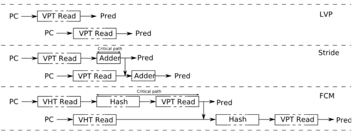
Figure 1: Prediction flow and critical paths for different value predictors when two occurrences of an instruction are fetched in two consecutive cycles.
Validation at Execution Time vs. Validation at Commit Time On the one hand,
selec-tive reissue must be implemented at execution time in order to limit the misprediction penalty.
On the other hand, pipeline squashing can be implemented either at execution time or at commit time. Pipeline squashing at execution time results in a minimum misprediction penalty similar to the branch misprediction penalty. However, validating predictions at execution time necessitates to redesign the complete out-of-order engine: the predicted values must be propagated through all the out-of-execution engine stages and the predicted results must be validated as soon as
they are produced in this out-of-order execution engine. Moreover, the repair mechanism must be able to restore processor state for any predicted instruction,Moreover, prediction checking must also be implemented in the commit stage(s) since predictors have to be trained even when predictions were not used due to low confidence.
On the contrary, pipeline squashing at commit results in a quite high average misprediction penalty since it can delay prediction validation by a substantial number of cycles. Yet, it is much easier to implement for Value Prediction since it does not induce complex mechanisms in the out-of-order execution engine. It essentially restrains the Value Prediction related hardware to the in-order pipeline front-end (prediction) and the in-order pipeline back-end (validation and training). Moreover, it allows not to checkpoint the rename table since the committed rename map contains all the necessary mappings to restart execution in a correct fashion.
A Simple Synthetic Example Realistic estimations of the average misprediction penalty
Pvalue could be 5-7 cycles for selective reissue1, 20-30 cycles for pipeline squashing at execution
time and 40-50 cycles for pipeline squashing at commit.
For the sake of simplicity, we will respectively use 5, 20 and 40 cycles in the small example that follows. We assume a benefit of 0.3 cycles per correctly predicted value. With predictors achieving around 40% coverage and around 95% accuracy as often reported in the literature, 50% of predictions used before execution, the performance benefit when using selective reissue would be around 64 cycles per Kinstructions, a loss of around 86 cycles when using pipeline squashing at execution time and a loss of around 286 cycles when using pipeline squashing at commit time. Our experiments in Section 8 confirm that when a value predictor exhibits a few percent misprediction rate on an application, it can induce significant performance loss when using pipeline squashing. Therefore, such a predictor should rather be used in conjunction with selective reissue.
3.1.2 Balancing Accuracy and Coverage
The total misprediction penalty Trecov is roughly proportional to the number of mispredictions.
Thus, if one drastically improves the accuracy at the cost of some coverage then, as long as the coverage of the predictor remains quite high, there might be a performance benefit of using Value Prediction, even though the average value misprediction penalty is very high.
Using the same example as above, but sacrificing 25% of the coverage (now only 30%), and assuming 99.75% accuracy, the performance benefit would be around 88 cycles per Kinstructions cycles when using selective reissue, 83 cycles when using pipeline squashing at execution time and 76 cycles when using pipeline squashing at commit time.
In Section 8, we will show that the ranges of accuracy and coverage allowed by our FPC proposition are in the range of those used in this small example. As a consequence, it is not surprising that our experiments confirm that, using FPC, pipeline squashing at commit time achieves performance in the same range as an idealistic 0-cycle selective reissue implementation.
3.2
Back-to-back prediction
Unlike a branch prediction, a value prediction is needed rather late in the pipeline (at dispatch time). Thus, at first glance, prediction latency does not seem to be a concern and long lookups in large tables and/or fairly complex computations could be tolerated. However, for most predictors,
1
including tracking and canceling the complete chain of dependent instructions as well as the indirect sources of performance loss encountered such as resource contention due to reexecution, higher misprediction rate (e.g. a value predicted using wrong speculative value history) and lower prediction coverage
the outcomes of a few previous occurrences of the instruction are needed to perform a prediction for the current instance. Consequently, for those predictors, either the critical operation must be made short enough to allow for the prediction of close (possibly back-to-back) occurrences (e.g. by using small tables) or the prediction of tight loops must be given up. Unfortunately, tight loops with candidates for VP are quite abundant in existing programs. Experiments conducted with the methodology we will introduce in Section 7 suggest that for a subset of the SPEC’00/’06 benchmark suites, there can be as much as 15.3% (3.4% a-mean) fetched instructions eligible for VP and for which the previous occurrence was fetched in the previous cycle (8-wide Fetch). We highlight such critical operations for each predictor in the subsequent paragraphs.
LVP Despite its name, LVP does not require the previous prediction to predict the current
instance as long as the table is trained. Consequently, LVP use only the program counter to generate a prediction. Thus, successive table lookups are independent and can last until Dispatch, meaning that large tables can be implemented. The top part of Fig. 1 describes such behavior. Similarly, the predictor we introduce in Section 6 only uses control-flow information to predict, allowing it to predict back-to-back occurrences. The same goes for the gDiff predictor itself [26] although a critical path may be introduced by the predictor providing speculative values for the global history.
Stride The prediction involves using the result of the previous occurrence of the instruction.
Thus, tracking the result of only the last speculative occurrence of the instruction is sufficient. The Stride value predictor acts in two pipeline steps, 1) retrieval of the stride and the last value 2) computation of the sum. The first step induces a difficulty when the last occurrence of the instruction has not committed or is not even executed. One has to track the last occurrence in the pipeline and use the speculative value predicted for this occurrence. This tracking can span over several cycles. The critical operation is introduced by the need to bypass the result of the second step directly to the adder in case of fetching the same instruction in two consecutive cycles (e.g. in a very tight loop), as illustrated by the central part of Fig. 1. However, a Stride value predictor supporting the prediction of two consecutive occurrences of the same instruction one cycle apart could reasonably be implemented since the second pipeline step is quite simple.
Finite Context Method The local value history predictor (nth-order FCM) is a two-level
structure. The first-level consists of a value history table accessed using the instruction address. This history is then hashed and used to index the second level table.
As for the Stride value predictor, the difficulty arises when several occurrences of the same instruction are fetched in a very short interval since the predictor is indexed through a hash of the last n values produced by the instruction. In many cases, the previous occurrences of the instruction have not been committed, or even executed. The logic is slightly more complex than for the stride predictor since one has to track the last n values instead of a single one.
However, the critical delay is on the second step. The delay between the accesses to the second level table for two occurrences of the same instruction is much shorter than the delay for computing the hash, reading the value table and then forward the predicted value to the second index hash/computation, as illustrated by the bottom part of Fig. 1. This implies that FCM must either use very small tables to reduce access time or give up predicting tight loops. Note that D-FCM [8] and DDISC [22] also require two successive lookups. Consequently, these observations stand for those predictors.
In summary, a hardware implementation of a local history value predictor would be very complex since 1) it involves tracking the n last speculative occurrences of each fetched instruction 2) the predictor cannot predict instructions in successive iterations of a loop body if the body is
fetched in a delay shorter than the delay for retrieving the prediction and forwarding it to the VPT index computation step.
Summary Table lookup time is not an issue as long as the prediction arrives before Dispatch
for LVP and Stride. Therefore, large predictor tables can be considered for implementation. For Stride-based value predictor, the main difficulty is that one has to track the last (possibly speculative) occurrence of each instruction.
For local value based predictors the same difficulty arises with the addition of tracking the
n last occurrences. Moreover the critical operations (hash and the 2nd level table read) lead
to either using small tables or not being able to timely predict back-to-back occurrences of the same instruction. Implementations of such predictors can only be justified if they bring significant performance benefit over alternative predictors.
The VTAGE predictor we introduce in this paper is able to seamlessly predict back-to-back occurrences of the same instruction, thus its access can span over several cycles. VTAGE does not require any complex tracking of the last occurrences of the instruction. Section 8 shows that VTAGE (resp. hybrid predictor using VTAGE) outperforms a local value based FCM predictor (resp. hybrid predictor using a local value based FCM predictor).
4
Commit Time Validation and Hardware Implications on
the Out-of-Order Engine
In the previous section, we have pointed out that the hardware modifications induced by pipeline
squashing at commit time on the Out-of-Order engine are limited. In practice, the only major
modification compared with a processor without Value Prediction is that the predicted values must be written in the physical registers before Dispatch.
At first glance, if every register has to be predicted for each fetch group, one would conclude that the number of write ports should double. In that case the overhead on the register file would be quite high. The area cost of a register file is approximately proportional to (R+W )∗(R+2W ),
Rand W respectively being the number of read ports and the number of write ports. Assuming
R = 2W , the area cost without value prediction would be proportional to 12W2
and the one
with value prediction would be proportional to 24W2
, i.e. the double. Energy consumed in the register file would also be increased by around 50% (using very simple Cacti 5.3 approximation). For practical implementations, there exist several opportunities to limit this overhead. For instance one can limit the number of extra ports needed to write predictions. Each cycle, only a few predictions are used and the predictions can be known several cycles before Dispatch: one could limit the number of writes on each cycle to a certain limit, and buffer the extra writes,
if there are any. Assuming only W
2 write ports for writing predicted values leads to a register
file area of 35W2
2 , saving half of the overhead of the naive solution. The same saving on energy
is observed (Cacti 5.3 estimations). Another opportunity is to allocate physical registers for consecutive instructions in different register file banks, limiting the number of write ports on the individual banks. One can also prioritize the predictions according to the criticality of the instruction and only use the most critical one, leveraging the work on criticality estimation of Fields et al. [6], Tune et al. [24] as well as Calder et al. [3].
Exploring the complete optimization to reduce the overhead on the register file design is out of the scope of this paper. It would depend on the precise micro-architecture of the processor, but we have clearly shown that this overhead in terms of energy and silicon area can be reduced to less than 25% and 50% respectively. Moreover, this overhead is restricted to the register file and does not impact the other components of the Out-of-order engine. Similarly, thanks to commit
time validation, the power overhead introduced by Value Prediction will essentially reside in the predictor table.
5
Maximizing Value Predictor Accuracy Through
Confi-dence
As we already pointed out, the total misprediction recovery cost can be minimized through two vehicles: minimizing the individual misprediction penalty and/or minimizing the total number of mispredictions.
When using the prediction is not mandatory (i.e. contrarily to branch predictions), an efficient way to minimize the number of mispredictions is to use saturating counter to estimate confidence and use the prediction only when the associated confidence is very high. For instance, for the value predictors considered in this study, a 3-bit confidence counter per entry that is reset on each misprediction leads to an accuracy in the 95-99% range if the prediction is used only when the counter is saturated. However this level of accuracy is still not sufficient to avoid performance loss in several cases unless idealistic speculative reissue is used.
We actually found that simply using wider counters (e.g. 6 or 7 bits) leads to much more accurate predictors while the prediction coverage is only reduced by a fraction. Prediction is only used on saturated confidence counters and counters are reset on each misprediction. Interestingly, probabilistic 3-bit counters such as defined by Riley et al. [15] augmented with reset on misprediction achieve the same accuracy for substantially less storage and a marginal increase in complexity.
We refer to these probabilistic counters as Forward Probabilistic Counters (FPC). In par-ticular, each forward transition is only triggered with a certain probability. In this paper, we
will consider 3-bit confidence counters using a probability vector v = {1, 1
16, 1 16, 1 16, 1 16, 1 32, 1 32}
for pipeline squashing at commit and v = {1,1
8, 1 8, 1 8, 1 8, 1 16, 1
16} for selective reissue, respectively
mimicking 7-bit and 6-bit counters. This generally prevents all the considered VP schemes to slow down execution while minimizing the loss of coverage (as opposed to using lower probabilities). The used pseudo-random generator is a simple Linear Feedback Shift Register.
Using FPC counters instead of full counters limits the overhead of confidence estimation. It also opens the opportunity to adapt the probabilities at run-time as suggested in [19] and/or to individualize these probabilities depending on the criticality of the instructions.
6
The Value TAgged GEometric Predictor
Branch predictors exploiting correlations inside the global branch history have been shown to be efficient. Among these global history branch predictors, TAGE [20] is generally considered state-of-the-art. An indirect branch predictor ITTAGE [20] has been directly derived from TAGE. Since targets of indirect branches are register values, we have explored the possibility of adapting ITTAGE to Value Prediction. We refer to this modified ITTAGE as the Value TAgged GEometric history length predictor, VTAGE. To our knowledge, VTAGE is the first hardware value predictor to make extensive use of recent and less recent control-flow history. In particular, PS [14] only uses a few bits of the global branch history.
As it uses branch history to predict, we expect VTAGE to perform much better than other pre-dictors when instruction results are indeed depending on the control flow. Nonetheless, VTAGE is also able to capture control-flow independent patterns as long as they are short enough with regard to the maximum history length used by the predictor. In particular, it can still capture
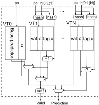
Figure 2: (1+N)-component VTAGE predictor. Val is the prediction, c is the hysteresis counter acting as confidence counter, u is the useful bit used by the replacement policy to find an entry to evict if required.
short strided patterns, although space efficiency is not optimal since each value of the pattern will reside in an entry (contrarily to the Stride predictor where one pattern can be represented by a single entry, for instance).
Fig. 2 describes a (1+N)-component VTAGE predictor. The main idea of the VTAGE scheme (exactly like the ITTAGE scheme) is to use several tables – components – storing predictions. Each table is indexed by a different number of bits of the global branch history, hashed with the PC of the instruction. The different lengths form a geometric series. These tables are backed up by a base predictor – a tagless LVP predictor – which is accessed using the instruction address only. In VTAGE, an entry of a tagged component consists of a partial tag, a 1-bit usefulness counter u used by the replacement policy, a full 64-bit value val, and a confidence/hysteresis counter c. An entry of the base predictor simply consists of the prediction and the confidence counter.
At prediction time, all components are searched in parallel to check for a tag match. The matching component accessed with the longest history is called the provider component as it will provide the prediction to the pipeline.
At update time, only the provider is updated. On either a correct or an incorrect prediction,
ctr2and u3are updated. On a misprediction, val is replaced if ctr is equal to 0, and a new entry
is allocated in a component using a longer history than the provider : all “upper” components are accessed to see if one of them has an entry that is not useful (u is 0). If none is found, the
u counter of all matching entries are reset but no entry is allocated. Otherwise, a new entry is
allocated in one of the components whose corresponding entry is not useful. The component is chosen randomly.
2
c= c + 1if correct or c − 1 if incorrect. Saturating arithmetic.
3
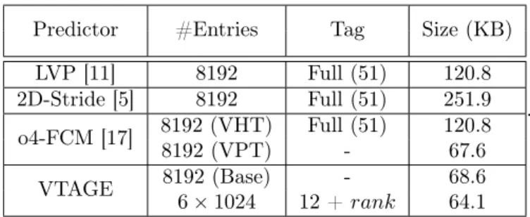
Predictor #Entries Tag Size (KB) LVP [11] 8192 Full (51) 120.8 2D-Stride [5] 8192 Full (51) 251.9 o4-FCM [17] 8192 (VHT) Full (51) 120.8 8192 (VPT) - 67.6 VTAGE 8192 (Base) - 68.6 6 × 1024 12 + rank 64.1 .
Table 1: Layout Summary. For VTAGE, rank is the position of the tagged component and varies from 1 to 6.
The main difference between VTAGE and ITTAGE is essentially the usage: the predicted value is used only if its confidence counter is saturated. We refer the reader to [20] for a more detailed description of ITTAGE.
Lastly, as a prediction does not depend on previous values but only on previous control-flow, VTAGE can seamlessly predict instructions in tight loops and behaves like LVP in Fig. 1. However, due to index hash and multiplexing from multiple components, it is possible that its prediction latency will be higher, although this is unlikely to be an issue since it has several cycles to predict.
7
Evaluation Methodology
7.1
Value Predictors
7.1.1 Single Scheme Predictors
We study the behavior of several distinct value predictors in addition to VTAGE. Namely, LVP [11], the 2-delta Stride predictor (2D-Stride) [5] as a representative of the stride-based predictor
family4 and a generic order-4 FCM predictor (o4-FCM) [17].
One could argue that we disregard D-FCM while it is more efficient than FCM. This is because VTAGE can be enhanced in the same way as FCM and it would be more fair to compare D-FCM against such a predictor rather than the baseline VTAGE. We leave such a comparison for future work.
All predictors use 3-bit saturating counters as confidence counters. The prediction is used only if the confidence counter is saturated. Baseline counters are incremented by one on a correct prediction and reset on a misprediction. The predictors were simulated with and without FPC (See Section 5). As the potential of VP has been covered extensively in previous work, we limit ourselves to reasonably sized predictors to gain more concrete insights. We start from a 128KB LVP (8K-entry) and derive the other predictors, each of them having 8K entries as we wish to gauge the prediction generation method, not space efficiency. Predictor parameters are illustrated in Table 1.
For VTAGE, we consider a predictor featuring 6 tables in addition to a base component. The base component is a tagless LVP predictor. We use a single useful bit per entry in the tagged components and a 3-bit hysteresis/confidence counter c per entry in every component. The tag of tagged components is 12+rank -bit long with rank varying between 1 and 6. The minimum
4
To save space, we do not illustrate the Per-Path Stride predictor [14] that we initially included in the study. Performance were on-par with 2D-Str.
and maximum history lengths are respectively 2 and 64 as we found that these values provided a good tradeoff in our experiments.
For o4-FCM, we use a hash function similar to those described in [18] and used in [8]: for a
nthorder predictor, we fold (XOR) each 64-bit history value upon itself to obtain a 16-bit index.
Then, we XOR the most recent one with the second most recent one left-shifted by one bit, and so on. Even if it goes against the spirit of FCM, we XOR the resulting index with the PC in order to break conflicts as we found that too many instructions were interfering with each other in the VPT. Similarly, we keep a 2-bit hysteresis counter in the VPT to further limit replacements (thus interference). This counter is incremented if the value matches the one already present, and decremented if not. The value is replaced only if the counter is 0.
We consider that all predictors are able to predict instantaneously. As a consequence, they can seamlessly deliver their prediction before Dispatch. This also implies that o4-FCM is – unrealistically – able to deliver predictions for two occurrences of the same instruction fetched in two consecutive cycles. Hence, its performance is most likely to be overestimated.
7.1.2 Hybrid Predictors
We also report numbers for a simple combination of VTAGE/2D-Str and o4-FCM/2D-Str, using the predictors described in Table 1. To select the prediction, we use a very simple mechanism: If only one component predicts (i.e. has high confidence), its prediction is naturally selected. When both predictors predict and if they do not agree, no prediction is made. If they agree, the prediction proceeds. Our hybrids also use the prediction of a component as the speculative last occurrence used by another component to issue a prediction (e.g. use the last prediction of VTAGE as the next last value for 2D-Stride if VTAGE is confident). When a given instruction retires, all components are updated with the committed value. To obtain better space efficiency, one can use a dynamic selection scheme such as the one Rychlik et al. propose. They assign a prediction to one component at most [16].
For the sake of clarity, we do not study gDiff [26] and DDISC [22] but we point out that they can be added "on top" of any other predictor. In particular, a hybrid of VTAGE and Stride, which, contrarily to FCM or any hybrid featuring FCM, would be feasible.
7.2
Simulator
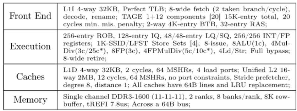
Front End L1I 4-way 32KB, Perfect TLB; 8-wide fetch (2 taken branch/cycle),decode, rename; TAGE 1+12 components [20] 15K-entry total, 20
cycles min. mis. penalty; 2-way 4K-entry BTB, 32-entry RAS;
Execution
256-entry ROB, 128-entry IQ, 48/48-entry LQ/SQ, 256/256 INT/FP registers; 1K-SSID/LFST Store Sets [4]; 8-issue, 8ALU(1c), 4Mul-Div(3c/25c*), 8FP(3c), 4FPMulDiv(5c/10c*), 4Ld/Str; Full bypass; 8-wide retire;
Caches L1D 4-way 32KB, 2 cycles, 64 MSHRs, 4 load ports; Unified L2 16-way 2MB, 12 cycles, 64 MSHRs, no port constraints, Stride prefetcher,
degree 8, distance 1; All caches have 64B lines and LRU replacement;
Memory Single channel DDR3-1600 (11-11-11), 2 ranks, 8 banks/rank, 8K row-buffer, tREFI 7.8us; Across a 64B bus;
Table 2: Simulator configuration overview. *not pipelined.
In our experiments, we use the gem5 cycle-accurate simulator (x86 ISA) [2]. We model a fairly aggressive pipeline: 4GHz, 8-wide superscalar, out-of-order processor with a latency of 19 cycles. We chose a slow front-end (15 cycles) coupled to a swift back-end (3 cycles) to obtain
a realistic misprediction penalty. Table 2 describes the characteristics of the pipeline we use in more details. As µ-ops are known at Fetch in gem5, all the width given in Table 2 are in µ-ops, even for the fetch stage. Independent memory instructions (as predicted by the Store Set predictor [4]) are allowed to issue out-of-order. Entries in the IQ are released upon issue (except with selective reissue). Since accuracy is high, branches are resolved on data-speculative paths [21].
The predictor makes a prediction at Fetch for every µ-op (we do not try to estimate criticality or focus only on load instructions) producing a register explicitly used by subsequent µ-ops. In particular, branches are not predicted with the value predictor but values feeding into branch instructions are. To index the predictors, we XOR the PC of the x86 instruction left-shifted by two with the µ-op number inside the x86 instruction to avoid all µ-ops mapping to the same entry. This mechanism ensures that most µ-ops of a macro-op will generate a different predictor index and therefore have their own entry in the predictor. We assume that the predictor can deliver as many predictions as requested by the Fetch stage. A prediction is written into the register file and replaced by its non-speculative counterpart when it is computed. However, a real implementation of VP need not use this exact mechanism, as discussed in Section 4.
Program Input
164.gzip (INT) input.source 60
168.wupwise (FP) wupwise.in
173.applu (FP) applu.in
175.vpr (INT) net.in arch.in place.out dum.out -nodisp -place_only -init_t 5 -exit_t
0.005 -alpha_t 0.9412 -inner_num 2
179.art (FP) -scanfile c756hel.in -trainfile1 a10.img -trainfile2 hc.img -stride 2 -startx 110 -starty 200 -endx 160 -endy 240 -objects 10
186.crafty (INT) crafty.in
197.parser (INT) ref.in 2.1.dict -batch
255.vortex (INT) lendian1.raw
401.bzip2 (INT) input.source 280
403.gcc (INT) 166.i 416.gamess (FP) cytosine.2.config 429.mcf (INT) inp.in 433.milc (FP) su3imp.in 444.namd (FP) namd.input 445.gobmk (INT) 13x13.tst 456.hmmer (INT) nph3.hmm
458.sjeng (INT) ref.txt
464.h264ref (INT) foreman_ref_encoder_baseline.cfg
470.lbm (FP) reference.dat
.
Table 3: Benchmarks used for evaluation. Top: CPU2000, Bottom: CPU2006. INT: 12, FP: 7, Total: 19.
7.2.1 Misprediction Recovery
We illustrate two possible recovery scenarios, squashing at commit time and a very idealistic selective reissue. In both scenarios, recovery is unnecessary if the prediction of instruction I was wrong but no dependent instruction has been issued before the execution of I, since the
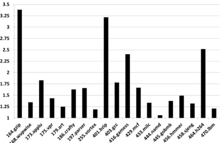
1 1.25 1.5 1.75 2 2.25 2.5 2.75 3 3.25 3.5
Figure 3: Speedup upper bound for the studied configurations. An oracle predicts all results.
prediction is replaced by the effective result at execution time. This removes useless squashes and is part of our implementation.
For selective reissue, we assume an idealistic mechanism where repair is immediate. All value speculatively issued instructions stay in the IQ until they become non speculative (causing more pressure on the IQ). When a value misprediction is found, the IQ and LSQ are searched for dependents to reissue. Ready instructions can be rescheduled in the same cycle with respect to the issue width.
Yet, even such an idealistic implementation of selective reissue does not only offer performance advantages. In particular, it can only inhibit an entry responsible for a wrong prediction at update time. Consequently, in the case of tight loops, several occurrences of the same instruction can be inflight, and a misprediction for the first occurrence will often result in mispredictions for subsequent occurrences, causing multiple reissues until the first misprediction retires.
The 0-cycle reissue mechanism is overly optimistic because of the numerous and complex steps selective reissue implies. Our experiments should be considered as the illustration that even a perfect mechanism would not improve significantly performance compared with squashing at commit time as long as value prediction is very accurate.
7.3
Benchmark Suite
We use a subset of the the SPEC’00 and SPEC’06 suites to evaluate our contributions as we focus on single-thread performance. Specifically, we use 12 integer benchmarks and 7 floating-point
programs5. Table 3 summarizes the benchmarks we use as well as their input, which are part
of the reference inputs provided in the SPEC software packages. To get relevant numbers, we identify a region of interest in the benchmark using Simpoint 3.2. We simulate the resulting slice in two steps: 1) Warm up all structures (Caches, branch predictor and value predictor) for 50M instructions, then collect statistics (Speedup, coverage, accuracy) for 50M instructions.
5
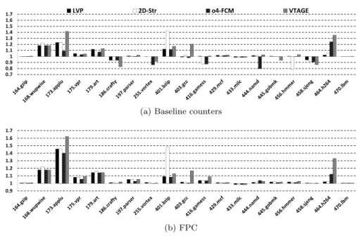
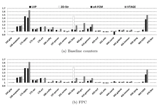
0.7 0.8 0.9 1 1.1 1.2 1.3 1.4 1.5 1.6 1.7 LVP 2D-Str o4-FCM VTAGE
(a) Baseline counters
0.9 1 1.1 1.2 1.3 1.4 1.5 1.6 1.7 (b) FPC
Figure 4: Speedup over baseline for different predictors using the squashing at commit mechanism to recover from a value misprediction.
8
Simulation Results
8.1
Potential benefits of Value Prediction
We first run simulations to assess the maximum benefit that could be obtained by a perfect value predictor. That is, performance is limited only by fetch bandwidth, memory hierarchy behavior, branch prediction behavior and various structure sizes (ROB, IQ, LSQ).
Fig. 3 shows that a perfect predictor would indeed increase performance by quite a significant amount (up to 3.3) in most benchmarks.
8.2
General Trends
8.2.1 Forward Probabilistic Counters
Fig. 4 illustrates speedup over baseline using squashing at commit to repair a misprediction. First, Fig. 4 (a) suggests that the simple 3-bit counter confidence estimation is not sufficient. Accuracy is generally comprised between 0.94 and almost 1.0, yet fairly important slowdowns can be observed. Much better accuracy is attained using FPC (above 0.997 in all cases), and translates to performance gain when using VP. Only milc is slightly slowed down, but this is considered acceptable as slowdown is smaller than 1%. This demonstrates that by pushing accuracy up, VP yields performance increase even with a pessimistic – but much simpler – recovery mechanism.
8.2.2 Prediction Coverage and Accuracy
Accuracy of predictions when using FPC is widely improved with accuracy being higher than 0.997 for every benchmark. This accuracy improvement comes at some reduction of the predictor coverage, especially for applications for which the accuracy of the baseline predictor was not
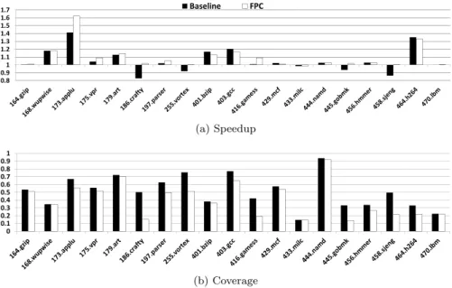
0.8 0.9 1 1.1 1.2 1.3 1.4 1.5 1.6 1.7 Baseline FPC (a) Speedup 0 0.1 0.2 0.3 0.4 0.5 0.6 0.7 0.8 0.9 1 (b) Coverage
Figure 5: Speedup and coverage of VTAGE with and without FPC. The recovery mechanism is
squashing at commit.
that high. This is illustrated in Fig. 5 for VTAGE: the greatest losses of coverage correspond to the applications that have the lowest baseline accuracy, i.e. crafty, vortex, gamess, gobmk, sjeng. These applications are also those for which a performance loss was encountered for the baseline while no performance is lost with FPC, i.e. crafty, vortex, gobmk, sjeng. For applications already having high accuracy and showing performance increase with the baseline, coverage is also slightly decreased, but in a more moderate way. Similar behaviors are encountered for the other predictors.
Note that high coverage does not correlate with high performance, e.g. namd exhibits 90% coverage but marginal speedup since there does not exist potential to speedup the application through value prediction (see Fig. 3). On the other hand, a small coverage may lead to significant speed-up e.g. h264.
8.2.3 Prediction schemes
Fig. 4 (b) shows that from a performance standpoint, no single-scheme predictor plainly out-performs the others even though some benchmarks achieve higher performance with 2D-Stride (wupwise and bzip) or VTAGE (applu, gcc, gamess and h264 ). This advocates for hybridization. Nonetheless, if VTAGE is outperformed by computational predictors in some cases, it gener-ally appears as a simpler and better context-based predictor than our implementation of o4-FCM. In our specific case, o4-FCM suffers mostly from a lack of coverage stemming from the use of a stricter confidence mechanism and from needing more time to learn patterns.
8.2.4 Pipeline Squashing vs. Selective Reissue
Fig. 6 illustrates experiments similar to those of Fig. 4 except selective reissue is used to repair a value misprediction. On the one hand, selective reissue significantly decreases the mispredic-tion penalty, therefore, performance gain is generally obtained even without FPC because less
0.9 1 1.1 1.2 1.3 1.4 1.5 1.6 1.7 LVP 2D-Str o4-FCM VTAGE
(a) Baseline counters
0.9 1 1.1 1.2 1.3 1.4 1.5 1.6 1.7 (b) FPC
Figure 6: Speedup over baseline for different predictors using selective reissue to recover from a value misprediction.
coverage is lost due to the confidence estimation scheme. Yet, this result has to be pondered by the fact that our implementation of selective reissue is idealistic.
On the other hand, with FPC, we observe that the recovery mechanism has little impact since the speedups are very similar in Fig. 4 (b) and Fig. 6 (b). In other words, provided that a confidence scheme such as ours yields very high accuracy, even an optimistic implementation of a very complex recovery mechanism will not yield significant performance increase. It is only if such confidence scheme is not available that selective reissue becomes interesting, although Zhou et al. state that even a single-cycle penalty – which is more conservative than our implementation – can nullify speedup if accuracy is too low (under 85%) [27].
Lastly, one can observe that performance with selective reissue is lower than with pipeline
squashing at commit in some cases even with FPC (e.g. art with o4-FCM). This is due to
consecutive mispredictions as discussed in Section 7.
8.3
Hybrid predictors
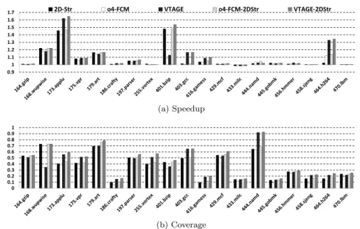
For the sake of readability, we only report results for the squashing recovery mechanism, but trends are similar for selective reissue.
Fig. 7 (a) illustrates speedups for a combination of VTAGE and 2D-Stride as well as o4-FCM and 2D-Stride. As expected, simple hybrids yield slightly higher performance than single predic-tor schemes, generally achieving performance at least on par with the best of the two predicpredic-tors. However, improvement over this level is generally marginal. Also note that computational and context-based predictors (in particular, VTAGE and Stride) indeed predict different instructions since coverage is generally increased, as shown by Fig. 7 (b).
Nonetheless, VTAGE + 2D-Stride appears as a better combination than o4-FCM + 2D-Stride, in addition to being simpler to implement.
0.9 1 1.1 1.2 1.3 1.4 1.5 1.6
1.7 2D-Str o4-FCM VTAGE o4-FCM-2DStr VTAGE-2DStr
(a) Speedup 0 0.1 0.2 0.3 0.4 0.5 0.6 0.7 0.8 0.9 1 (b) Coverage
Figure 7: Speedup over baseline and coverage of a 2-component symmetric hybrid made of 2D-Stride and VTAGE with FPC. Squashing at commit is the recovery mechanism.
9
Conclusion
To our knowledge, Value Prediction has not been considered for current commercially-available microprocessors. However, as the number of cores in high-end processors has now reached the 8-16 range, there is a new call for enhancing core performance rather than increasing the number of cores. Given the availability of a large number of transistors, Value Prediction appears as a good candidate to further increase performance. In this paper, we reconsidered Value Prediction in this new context.
In particular, the two propositions presented in this paper may favor the practical implemen-tation of Value Prediction in the future generation processors.
First, we have shown that the use of value prediction can be effective, even if the prediction validation is performed at commit time. Using probabilistic saturating confidence counters with a low increment probability can greatly benefit any value predictor: a very high accuracy (> 99.5%) can be ensured for all existing value predictors at some cost in coverage, using very simple hardware. Very high accuracy is especially interesting because it allows to tolerate the high individual average misprediction associated with validation at commit time. In this context, complex recovery mechanisms such as selective reissue has very marginal performance interest. In other words, we claim that, granted a proper confidence estimation mechanism such as the FPC scheme, state-of-the art value predictors can improve performance on a fairly wide and deep pipeline while the prediction validation is performed at commit time. In this case, the value prediction hardware is essentially restricted to the in-order front-end (prediction) and the in-order back-end (validation and training) and the modifications to the out-of-order engine are very limited.
Second, we have introduced a new context-based value predictor, the Value TAGE predictor. We directly derived VTAGE from the ITTAGE predictor by leveraging the similarities between Indirect Branch Target Prediction and Value Prediction. VTAGE uses the global branch history as well as the path history to predict values. We have shown that it outperforms previous generic
context-based value predictors leveraging per-instruction value history (FCM). Moreover, a ma-jor advantage of VTAGE is its tolerance to high latency. In particular, it has to be contrasted with local value history based predictors as they suffer from long critical operation when pre-dicting consecutive instances of the same instruction. They are therefore highly sensitive to the prediction latency and cannot afford long lookup times, hence large tables. On the contrary, the access to VTAGE tables can span over several cycles (from Fetch to Dispatch) and VTAGE can be implemented using very large tables.
Through combining our two propositions, a practical hybrid value predictor can achieve fairly significant performance improvements while only requiring limited hardware modifications to the out-of-order execution engine. Our experiments show that while performance might be limited many applications – less than 5% on 10 out of 19 benchmarks –, encouraging performance gains are encountered on most applications – from 5% up to 65% on the remaining 9 benchmarks.
Acknowledgement
This work was partially supported by the European Research Council Advanced Grant DAL No 267175
References
[1] G.M. Amdahl, “Validity of the single processor approach to achieving large scale computing capabilities,” in Proceedings of the spring joint computer conference, April 18-20, 1967. ACM, 1967, pp. 483–485.
[2] N. Binkert, B. Beckmann, G. Black, S. K. Reinhardt, A. Saidi, A. Basu, J. Hestness, D. R. Hower, T. Krishna, S. Sardashti, R. Sen, K. Sewell, M. Shoaib, N. Vaish, M. D. Hill, and D. A. Wood, “The gem5 simulator,” SIGARCH Comput. Archit. News, vol. 39, no. 2, pp. 1–7, Aug. 2011.
[3] B. Calder, G. Reinman, and D.M. Tullsen, “Selective value prediction,” in Proceedings of
the International Symposium on Computer Architecture. IEEE, 1999, pp. 64–74.
[4] G. Z. Chrysos and J. S. Emer, “Memory dependence prediction using store sets,” in Proceedings of the 25th annual international symposium on Computer architecture, ser.
ISCA ’98. Washington, DC, USA: IEEE Computer Society, 1998, pp. 142–153. [Online].
Available: http://dx.doi.org/10.1145/279358.279378
[5] R.J. Eickemeyer and S. Vassiliadis, “A load-instruction unit for pipelined processors,” IBM Journal of Research and Development, vol. 37, no. 4, pp. 547–564, 1993.
[6] B. Fields, S. Rubin, and R. Bodík, “Focusing processor policies via critical-path prediction,” in Computer Architecture, 2001. Proceedings. 28th Annual International Symposium on. IEEE, 2001, pp. 74–85.
[7] F. Gabbay and A. Mendelson, “Using value prediction to increase the power of speculative execution hardware,” ACM Trans. Comput. Syst., vol. 16, no. 3, pp. 234–270, Aug. 1998. [8] B. Goeman, H. Vandierendonck, and K. De Bosschere, “Differential fcm: Increasing value
prediction accuracy by improving table usage efficiency,” in High-Performance Computer
Architecture, 2001. HPCA. The Seventh International Symposium on. IEEE, 2001, pp.
[9] M.D. Hill and M.R. Marty, “Amdahl’s law in the multicore era,” Computer, vol. 41, no. 7, pp. 33–38, 2008.
[10] I. Kim and M. H. Lipasti, “Understanding scheduling replay schemes,” in In International Symposium on High-Performance Computer Architecture, 2004, pp. 198–209.
[11] M.H. Lipasti and J.P. Shen, “Exceeding the dataflow limit via value prediction,” in
Pro-ceedings of the Annual International Symposium on Microarchitecture. IEEE Computer
Society, 1996, pp. 226–237.
[12] M.H. Lipasti, C.B. Wilkerson, and J.P. Shen, “Value locality and load value prediction,” ASPLOS-VII, 1996.
[13] A. Mendelson and F. Gabbay, “Speculative execution based on value prediction,” Technion-Israel Institute of Technology, Tech. Rep. TR1080, 1997.
[14] T. Nakra, R. Gupta, and M.L. Soffa, “Global context-based value prediction,” in Proceedings
of the International Symposium On High-Performance Computer Architecture, 1999. IEEE,
1999, pp. 4–12.
[15] N. Riley and C. B. Zilles, “Probabilistic counter updates for predictor hysteresis and strat-ification,” in Proceedings of the International Symposium on High Performance Computer Architecture, 2006, pp. 110–120.
[16] B. Rychlik, J.W. Faistl, B.P. Krug, A.Y. Kurland, J.J. Sung, M.N. Velev, and J.P. Shen, “Efficient and accurate value prediction using dynamic classification,” Carnegie Mellon Uni-versity, CMµART-1998-01, 1998.
[17] Y. Sazeides and J.E. Smith, “The predictability of data values,” in Proceedings of the Annual
International Symposium on Microarchitecture. IEEE, 1997, pp. 248–258.
[18] ——, “Implementations of context based value predictors,” Department of Electrical and Computer Engineering, University of Wisconsin-Madison, Tech. Rep. ECE97-8, 1998. [19] A. Seznec, “Storage free confidence estimation for the TAGE branch predictor,” in
Proceed-ings of the International Symposium on High Performance Computer Architecture, 2011. IEEE, 2011, pp. 443–454.
[20] A. Seznec and P. Michaud, “A case for (partially) tagged geometric history length branch prediction,” Journal of Instruction Level Parallelism, vol. 8, pp. 1–23, 2006.
[21] A. Sodani and G.S. Sohi, “Understanding the differences between value prediction and in-struction reuse,” in Proceedings of the Annual International symposium on Microarchitecture. IEEE Computer Society Press, 1998, pp. 205–215.
[22] R. Thomas and M. Franklin, “Using dataflow based context for accurate value prediction,” in Parallel Architectures and Compilation Techniques, 2001. Proceedings. 2001 International
Conference on. IEEE, 2001, pp. 107–117.
[23] D.M. Tullsen and J.S. Seng, “Storageless value prediction using prior register values,” in
Proceedings of the International Symposium on Computer Architecture. IEEE, 1999, pp.
[24] E. S. Tune, D. M. Tullsen, and B. Calder, “Quantifying instruction criticality,” in Parallel Architectures and Compilation Techniques, 2002. Proceedings. 2002 International
Confer-ence on. IEEE, 2002, pp. 104–113.
[25] K. Wang and M. Franklin, “Highly accurate data value prediction using hybrid predictors,” in Proceedings of the Annual International Symposium on Microarchitecture. IEEE Computer Society, 1997, pp. 281–290.
[26] H. Zhou, J. Flanagan, and T. M. Conte, “Detecting global stride locality in value streams,” in In Proceedings of the 30th Annual International Symposium on Computer Architecture. ACM Press, 2003, pp. 324–335.
[27] H. Zhou, C. Ying Fu, E. Rotenberg, and T. Conte, “A study of value speculative execution and misspeculation recovery in superscalar microprocessors,” Department of Electrical & Computer Engineering, North Carolina State University, pp.–23, Tech. Rep., 2000.
Campus universitaire de Beaulieu BP 105 - 78153 Le Chesnay Cedex inria.fr