Investigation on Near-field Source Localization and the Corresponding Applications

HAL Id: tel-01504375

https://hal.archives-ouvertes.fr/tel-01504375

Submitted on 10 Apr 2017

HAL is a multi-disciplinary open access archive for the deposit and dissemination of sci-entific research documents, whether they are pub-lished or not. The documents may come from teaching and research institutions in France or abroad, or from public or private research centers.

L’archive ouverte pluridisciplinaire HAL, est destinée au dépôt et à la diffusion de documents scientifiques de niveau recherche, publiés ou non, émanant des établissements d’enseignement et de recherche français ou étrangers, des laboratoires publics ou privés.

Public Domain

Corresponding Applications

Jianzhong Li

To cite this version:

Jianzhong Li. Investigation on Near-field Source Localization and the Corresponding Applications. Electronics. UNIVERSITE DE NANTES, 2017. English. �tel-01504375�

Thèse de Doctorat

Jianzhong L

I

Mémoire présenté en vue de l’obtention du

grade de Docteur de l’Université de Nantes

sous le sceau de l’Université Bretagne Loire

École doctorale Sciences et Technologies de l’Information et Mathématiques (STIM ED-503) Discipline : Electronique

Spécialité : Communications numériques Unité de recherche : IETR UMR 6164 Soutenue le 2 mars 2017

Investigation on Near-field Source Localization

and the Corresponding Applications

JURY

Président : M. Xianhua DAI, Professeur, Sun Yat-Sen University, Chine

Rapporteurs : M. Salah BOURENNANE, Professeur, Institut Fresnel, Ecole Centrale Marseille M. Zhilong SHAN, Professeur, South China Normal University

Directeur de thèse : M. Yide WANG, Professeur, Polytech Nantes, Université de Nantes

Co-directeur de thèse : M. Gang WEI, Professeur, South China University of Technology

Résumé étendu (Extended French Abstract)

Introduction

L’estimation de paramètres par méthode de traitement du signal est un sujet très important dans de nombreux domaines (radar, sismique, sonar, surveillance électronique, etc). Mes travaux de recherche se sont focalisés sur deux domaines de traitement du signal : le traitement d’antenne multi-capteurs et l’estimation des temps de retard.

Pour le traitement d’antenne multi-capteurs, je me suis focalisé sur la localisation de sources en champ proche. La localisation de sources a pour objectif d’estimer les paramètres de position des sources. La localisation de sources est largement appliquée dans de nombreux domaines (radar, sonar, télécom, etc), notamment avec l’aide de méthodes à sous-espace (MUSIC, ES-PRIT, MPM, etc). En champ lointain, une source est paramétrée seulement par sa direction d’arrivée (DDA). Quand les sources sont proches du réseau de capteurs (situation de champ proche), cette hypothèse n’est plus valide. En effet, dans ce cas, le front d’onde du signal est sphérique et deux paramètres sont alors nécessaires pour localiser les sources: la direction d’arrivée et la distance entre la source et le réseau de capteurs (Fig. 2-4).

Pour la localisation de sources en champ proche, de nombreux progrès sont encore attendus à ce jour, comme:

(1) la réduction de la complexité calculatoire des méthodes existantes, (2) l’amélioration de la résolution et de la précision des méthodes.

L’estimation des temps de retard est également largement appliquée dans de nombreux domaines (radar, sonar, ultra-son, etc). Dans le cadre de mes recherches, je me suis essentiellement fo-calisé sur l’estimation des temps de retard avec les radars géophysiques afin de déterminer les épaisseurs d’un milieu stratifié. Le radar géophysique permet de ≪ pointer ≫ les maximums des échos reçus. Il permet ainsi de déterminer les temps de retard des échos reçus afin d’évaluer par la suite les épaisseurs du milieu stratifié sondé. L’estimation des temps de retard est une ap-plication qui peut être considérée comme≪ proche ≫ des problématiques de traitement d’an-tenne car le modèle de signal utilisé dans ces deux applications est proche. Dans cette appli-cation, le signal reçu provient du même émetteur, ainsi les échos sont cohérents et donc les

de ≪ décorrélation ≫ des échos sont alors nécessaires. En outre, certains échos reçus par le radar géophysique peuvent être relativement faibles et il devient alors difficile d’interpréter les résultats, notamment dans un environnement bruité. Le challenge dans cette partie a été de pro-poser une méthode de traitement haute résolution et précise dans un environnement bruité, mais sans utiliser de méthode de≪ décorrélation ≫.

Depuis quelques années, les méthodes de≪ Compressive Sensing ≫ (CS) sont très populaires à l’international dans les domaines de la recherche et notamment dans les domaines des mathé-matiques appliquées, de l’informatique et du génie électrique. En théorie, ces méthodes per-mettent d’atteindre une résolution très élevée avec une très bonne précision et un nombre de mesures faible. De plus, elles peuvent aussi être utilisées sans prétraitement sur des signaux corrélés (comme des signaux provenant du radar géophysique).

De plus, depuis plusieurs années, les méthodes basées sur les statistiques d’ordre supérieur sont aussi très populaires, car elles permettent d’une part d’augmenter le degré de libertés des sig-naux reçus et d’autre part d’améliorer leur robustesse au bruit de nature gaussienne. En effet, leur intérêt est d’annuler l’influence du bruit gaussien, sous l’hypothèse d’observer un signal de sources non gaussiennes, additionné d’un bruit gaussien.

Ainsi, cette thèse a pour objectif de proposer et développer de nouvelles méthodes de traite-ment du signal rapides et efficaces basées sur des méthodes à sous-espace et/ou sur la théorie

≪ compressive sensing ≫, et/ou sur des statistiques d’ordre supérieur. Dans cette thèse, deux

applications sont investiguées: la première application consiste à localiser les sources en champ proche, la deuxième application, qui peut être considérée comme un cas particulier de la pre-mière application d’un point de vue ≪ traitement du signal ≫, consiste à estimer les temps de propagation des ondes électromagnétiques dans une chaussée. L’objectif de cette thèse est d’améliorer la précision, la résolution et le temps de calcul des méthodes de traitement du signal pour les applications envisagées.

Les méthodes proposées dans cette thèse sont évaluées en termes de résolution, du rapport signal sur bruit et du temps de calcul sur des signaux simulés et réels. Elles sont aussi comparées aux méthodes à sous-espaces de référence de la littérature comme par exemple MUSIC, ESPRIT….

Tout d’abord, le modèle de signal utilisé pour localiser les sources en champ lointain et en champ proche est présenté (section 2.2). De nombreuses recherches ont déjà été réalisées pour localis-er des sources en champ proche avec des méthodes à sous espace basées sur des statistiques de second ordre comme 2D-MUSIC par exemple. Pour la méthode haute résolution 2D-MUSIC, une recherche à deux dimensions est alors nécessaire (section 2.3.2). Ainsi, cette méthode pos-sède une complexité calculatoire très importante. Afin de réduire cette complexité calculatoire, la méthode≪ modified 2D-MUSIC ≫ propose d’utiliser les statistiques de second ordre pour construire une matrice ne contenant pas le paramètre lié à la≪ distance ≫ (section 2.3.3). Ain-si, ≪ modified 2D-MUSIC ≫ permet de réaliser une recherche monodimensionnelle pour es-timer seulement le paramètre DDA. Ensuite, une nouvelle matrice est construite pour eses-timer le deuxième paramètre: la distance. Cette méthode présente de très bons résultats et une complex-ité calculatoire plus faible que 2D-MUSIC. Comme indiqué dans l’introduction, les méthodes basées sur les statistiques d’ordre supérieur permettent d’une part d’augmenter le degré de lib-ertés des signaux reçus et d’autre part d’améliorer la robustesse au bruit de nature gaussienne. La notion d’ordre supérieur (cumulant) ainsi que ses propriétés sont présentées en détail dans la section 2.4.1. Puis, les méthodes≪ modified ESPRIT ≫ (section 2.4.2) et ≪ Modified 2D-MUSIC ≫ (section 2.4.3) qui ont aussi été proposées dans la littérature avec des statistiques d’ordre supérieur sont présentées. ≪ Modified 2D-MUSIC ≫ nécessite le calcul de deux ma-trices quand seulement une est nécessaire pour 2D-MUSIC. Enfin, la borne de Cramer-Rao pour la localisation de sources en champ proche est présentée dans la section 2.5.

Nouvelles méthodes à sous-espace basées sur les statistiques

d’ordre supérieur pour la localisation de sources en champ

proche

Dans ce chapitre, trois propositions d’amélioration de méthodes à sous-espace sont présentées dans le contexte de la localisation de sources en champ proche. Pour les applications avec des dispositifs avancés, dont la capacité de calcul peut être très importante, la complexité calcula-toire n’est pas un problème majeur. En revanche, pour des systèmes dont la puissance de calcul est limitée (système portatif par exemple), la complexité de calcul reste encore un enjeu majeur

La première proposition (section 3.3) est basée sur les statistiques d’ordre supérieur et est

insp-irée de la méthode ≪ Modified 2-D MUSIC ≫ (section 2.4.3). On montre que la méthode

MUSIC peut être appliquée avec une seule matrice cumulant (du quatrième ordre) non-Hermitienne. Ainsi, grâce à cette matrice spécifique, les DDA et les distances peuvent être estimées séparément. De plus, une seule décomposition en éléments propres est réalisée. Cette proposition permet ainsi de réduire la charge de calcul par comparaison avec la méthode≪ Mo-dified 2-D MUSIC ≫ basée sur les statistiques d’ordres deux et supérieur (section 3.2). Les résultats de simulation montrent que la méthode proposée possède presque les mêmes

perfor-mances que la méthode≪ Modified 2-D MUSIC ≫ (section 3.2), avec une complexité

calcu-latoire inférieure.

Ensuite (section 3.4), nous proposons d’utiliser une matrice cumulant dont les colonnes (lignes) peuvent aussi être définies comme la combinaison linéaire des colonnes (lignes) de deux ma-trices≪ modes ≫. Le sous-espace ≪ orthogonal ≫ au vecteur modèle peut alors être obtenu directement avec le principe du≪ propagateur ≫. Cette proposition est ensuite combinée avec la première amélioration. Ainsi, la décomposition en élément propre n’est plus nécessaire et la complexité calculatoire est davantage réduite.

Enfin (section 3.5), nous proposons d’agrandir virtuellement l’ouverture du réseau de capteurs afin d’améliorer la résolution et la précision dans l’estimation de la distance. Ainsi, une nou-velle matrice (de grande taille) est construite à partir des statistiques d’ordre supérieur. Puis, le principe développé en section 3.3 est utilisé afin de réduire la complexité de calcul.

Nouvelle méthode de

≪ compressive sensing ≫ basée sur les

statistiques d’ordre supérieur pour la localisation de sources

en champ proche

Dans ce chapitre, nous présentons tout d’abord la théorie du≪ Compressive Sensing ≫ (CS) (section 4.1). Ensuite, la localisation de sources en champ lointain basée sur la théorie du CS est présentée (section 4.2). Puis, nous proposons d’appliquer cette théorie pour la localisation

de sources en champ proche (section 4.3). Comme≪ Modified 2-D MUSIC ≫ (section 2.3.3),

Tout d’abord, une matrice spécifique basée sur les statistiques d’ordre supérieur est proposée, puis la reconstruction du signal basée sur la théorie CS est réalisée d’une part avec cette ma-trice spécifique et d’autre part avec sa transposée. Ainsi, la méthode proposée utilise seule-ment deux dictionnaires surdimensionnés 1D (au lieu d’un dictionnaire 2D surdimensionné) permettant ainsi d’estimer les deux paramètres séparément avec une charge de calcul faible. De plus, cette reconstruction contient aussi des informations pouvant être utilisées pour relier les deux paramètres provenant d’une même source. Ainsi, une méthode d’appariement basée sur la théorie du≪ clustering ≫, permettant d’exploiter pleinement la méthode CS, est proposée. Les simulations (section 4.4) ont montré que la méthode proposée possédait une meilleure résolution et une plus grande précision que les méthodes à sous-espace.

Application du radar géophysique dans un environnement

bruité

Dans ce chapitre, nous proposons d’améliorer la détection des interfaces de chaussée et l’estimation des épaisseurs d’un milieu stratifié par radar géophysique dans un contexte de faible Rapport Signal sur Bruit (RSB). Tout d’abord le modèle de signal (section 5.1) est présenté. Dans cette application, le signal reçu provient du même émetteur, ainsi les échos sont cohérents et donc les méthodes à sous-espace ne peuvent pas être appliquées directement. En effet, des algorithmes de≪ décorrélation ≫ des échos sont nécessaires. Une méthode de référence de

≪ décorrélation ≫ est alors présentée dans la section 5.2. De plus, certains échos reçus peuvent

être relativement faibles et il devient alors difficile d’interpréter les résultats, notamment dans un environnement bruité. Ainsi, dans ce chapitre, nous avons proposé tout d’abord une méthode pour améliorer le signal bruité reçu par le radar géophysique. Cette méthode présentée dans la section 5.3.1 est basée sur une méthode à sous-espace et sur une méthode de≪ clustering ≫. Ensuite, nous proposons d’utiliser le principe de CS sur ce nouveau signal afin d’estimer le temps de retard des échos rétrodiffusés (section 5.3.2). Cette méthode permet ainsi d’obtenir une résolution et une estimation plus précise que les méthodes à sous-espace, sans utiliser de méthode de≪ décorrélation ≫. Plusieurs simulations et une expérimentation sont présentées pour montrer l’efficacité de nos propositions (section 5.4).

L’objectif de cette thèse a été d’améliorer la précision, la résolution et le temps de calcul des méthodes de traitement du signal pour localiser des sources en champ proche ou pour estimer les temps de retard. Pour atteindre cet objectif, de nouvelles méthodes de traitement du signal basées sur des méthodes à sous-espace et/ou sur la théorie CS, et/ou sur des statistiques d’ordre supérieur, ont été proposées. L’efficacité des méthodes proposées a été évaluée par des simula-tions et des expérimentasimula-tions.

A l’issue de ce travail, plusieurs orientations peuvent être proposées comme perspectives. En matière d’amélioration de méthodes de localisation de sources en champ proche, nous proposons dans la continuité de cette thèse de:

• réduire la charge de calcul par des méthodes polynomiales (comme root-MUSIC par exemple);

• d’étendre les méthodes développées à des signaux large bande (dans cette thèse, seuls les signaux à bande étroite ont été utilisés);

• et d’étendre les méthodes lorsque les sources sont totalement corrélées.

Une autre perspective à moyen terme consisterait à tester ces méthodes de localisation de sources en champ proche avec des données réelles afin d’analyser leur comportement sur le terrain. Une dernière perspective concerne l’application de ces méthodes (localisation de sources et temps de retard) à l’imagerie radar géophysique 2D et 3D. De nombreuses autres problématiques du génie civil concernent la détection-localisation d’objets de dimensions réduites. L’extension des algorithmes à la détection de tels objets nécessite d’un modèle du signal 2D ou 3D prenant en compte la cohérence des sources. La redondance d’information existante d’un profil radar à l’autre (A-scan) pourrait aussi être exploitée.

Contents

Résumé étendu (Extended French Abstract) I

1 Introduction 1

1.1 Background and Motivation . . . 1

1.1.1 Background . . . 1

1.1.2 Problem Statement and Motivation . . . 3

1.2 Review of Source Localization . . . 5

1.3 Review of Compressive Sensing (CS) . . . 7

1.4 Review of Ground Penetrating Radar (GPR) . . . 9

1.5 Main Contributions . . . 10

1.6 Organization . . . 12

2 Modeling and Localizing Near-field Sources 14 2.1 Far-field Signal Model and the Corresponding Localization Methods . . . 14

2.1.1 Far-field Source Model . . . 15

2.1.2 Far-field Source localization . . . 16

2.2 Near-field Source Model . . . 21

2.3 Second-order Statistics Methods . . . 23

2.3.1 2D LP Estimator . . . 24

2.3.2 2D MUSIC . . . 25

2.3.3 Modified 2D MUSIC . . . 26

2.4 High-order Cumulant Methods . . . 28

2.4.1 High-order Cumulant . . . 28

2.4.2 ESPRIT-like Based On High-order Cumulant . . . 30

2.4.3 Modified 2D MUSIC based on High-Order Cumulant . . . 31

2.5 CRB . . . 33

3.1 Introduction . . . 36

3.2 Mix-order MUSIC for Near-field Source Localization . . . 36

3.3 Proposed Low-Complexity MUSIC (LCM) . . . 38

3.3.1 Signal Model . . . 39

3.3.2 DOA Estimation . . . 40

3.3.3 Range Estimation . . . 41

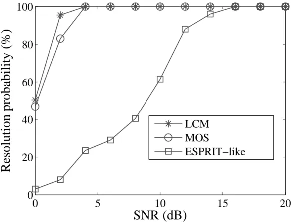
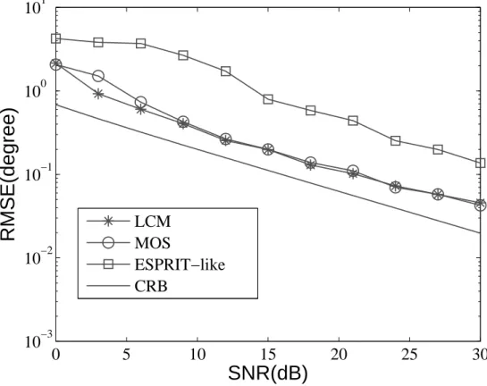
3.3.4 Simulation . . . 46

3.4 Proposed Propagator-based Method . . . 48

3.4.1 DOA Estimation . . . 51

3.4.2 Range Estimation . . . 52

3.4.3 Simulation . . . 53

3.5 Proposed Aperture-Expanded MUSIC (AEM) . . . 56

3.5.1 DOA Estimation . . . 57

3.5.2 Range Estimation . . . 58

3.5.3 Simulations . . . 60

3.6 Conclusion . . . 62

4 Joint DOA and Range Estimation based on Compressive Sensing 63 4.1 Introduction . . . 63

4.1.1 Orthogonal Matching Pursuit (OMP) . . . 64

4.1.2 ℓp_∈(0,1]Norm . . . 65

4.2 Far-field Source Localization based on Compressive Sensing . . . 67

4.2.1 ℓ1 Norm Optimization . . . 67

4.2.2 ℓ1-SVD . . . 68

4.3 Proposed CS-based Algorithm for Near-field Source Localization . . . 69

4.3.1 Estimation of Parameter ϕk . . . 70

4.3.2 Estimation of Parameter ωk . . . 71

4.3.3 Parameter Pairing . . . 73

5 GPR Applications in Low-SNR Scenario 80

5.1 Introduction and Signal Model . . . 80

5.2 Subspace-based Methods with SSP for TDE . . . 83

5.3 Proposed Algorithm for Time-delay Estimation in Low SNR . . . 85

5.3.1 Signal Enhancement . . . 85

5.3.2 Compressive Sensing for TDE . . . 87

5.4 Simulation and Experiment . . . 88

5.4.1 Simulation . . . 88

5.4.2 Experiment . . . 94

5.5 Conclusion . . . 95

6 Conclusion and Future Work 96 6.1 Conclusion . . . 96

6.2 Future work . . . 98

Bibliography 100

Publication 110

Chapter 1

Introduction

In this chapter, we begin by introducing the background and motivation for carrying out the source localization research. Then we review its development that has been achieved in the past decades. Compressive Sensing (CS, also called signal reconstruction), a newly proposed technique especially for source localization problems, will be specially introduced. As an ap-plication of source localization, the Ground Penetrating Radar (GPR) will also be reviewed. At last, we conclude our main contributions and present the organization of the dissertation.

1.1

Background and Motivation

1.1.1

Background

Signal processing is an important topic for modern communication technology. Traditional signal processing technology aims to deal with the information received by a single sensor. In recent decades, array signal processing has been attracting a lot of attention. Array signal processing considers the signals received by an array, which is made of several sensors in a specific configuration. This technology can enhance the target signal while minimizing the interference and noise. Compared to a single sensor, there are many advantages in the application of an array of sensors, such as spatial gain and resolution.

Nowadays, array signal processing has been widely applied and obtained many significant achievements in radar, sonar, communications, seismology and other fields.

(1) Radar is the field in which the antenna array is firstly used. In most cases, radar systems are active and the array is used to both transmit and receive signals.

(2) Sonar systems can be classified into active ones and passive ones. Active sonar systems are similar to active radar systems. A passive sonar system detects the incoming acoustic signals and gathers information to analyze their temporal and spatial characteristics.

(3) Satellite communication and territorial wireless communication concentrate on trans-mitting signals to specific users or receiving information from interested direction. Using an antenna array can help to focus the energy and minimize the interferences.

(4) In seismology, a geophone array is used to detect and locate the underground activities, such as nuclear explosion and earthquake. When an earthquake occurs, the epicenter can be measured and the underground medium can be analyzed with information gathered by the array.

In conclusion, array signal processing focuses mainly on the following problems:

(1) Signal separation, which aims to recover the individual signal from a mixture of several signals [1–3].

(2) Channel estimation, which aims to estimate the parameters of the channel between the source and the array [4, 5].

(3) Source localization, which aims to estimate the position parameters of the received signals.

(4) Spatial multiplexing, which aims to increase communication system capability.

(5) Spatial filtering, which aims to fix the main lobe at a desired direction and enhance the received signal.

(6) Interference rejection, which aims to form a beam null in the direction of the jamming to reduce and eliminate interference.

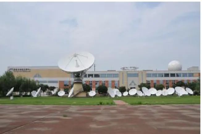
Source localization is becoming more and more attractive because of its wide range of ap-plications especially in radar, sonar and other detection techniques. Scholars from all over the world have been working hard into this topic for the past decades, and have proposed a lot of methods. The scope of its applications has been enlarged thanks to their effort. The develop-ment of source localization plays an important role in the national defense or the economic field [6]. The crack detection for architectures or railways relies heavily on the source localization technique [7]. Fig. 1-1 shows an array of sensors of a wireless signal monitoring center.

When a signal impinges on an array, there would be a phase difference among the received signals of different sensors, which contains enough information to determine the position of the signal source. Indeed, the phase difference can be modeled by the position parameters, leading to the feasibility to directly localize sources.

econom-Fig. 1-1 Wireless signal monitoring center

ical savings are surely two important factors. Subsurface deformations and cracks inside can cause sudden collapse, resulting in the fatal damage to the human lives and economical devel-opment. Therefore, detecting and monitoring the changes inside buildings or roads are of great importance. Among all the tools, the non-destructive ones attract, no doubt, the most attention. GPR is a non-destructive probing tool. Its main work is to carry out the Time-Delay Esti-mation (TDE) of the backscattered signal echoes, which are reflected by cracks or other damages inside the roads or buildings. The TDE is also a parameter estimation problem. Indeed, the sig-nal model is very similar to that of source localization. We can consider it as an application of source localization and many methods for source localization can be directly applied to the TDE with GPR.

1.1.2

Problem Statement and Motivation

For source localization, most of the algorithms have been developed to estimate the Direc-tion Of Arrival (DOA) of the signal sources under the assumpDirec-tion that the sources are in far-field. In this far-field case, the range of a source is far beyond the Fresnel region and the wavefront of signal is assumed to be a plane wave when it impinges the sensor array. Each source is parame-terized by only the DOA. However, in many cases, the sources are within the Fresnel region. In

this case, the plane wave assumption can no longer hold and the signal wavefronts are spherical. Both the DOAs and ranges will be necessary to localize these near-field sources, which would result in a more complicated problem. This dissertation mainly concentrates on the research in the near-field situation.

Basically, the most direct idea to localize near-field sources is to estimate the DOA and range of each source simultaneously. This idea inspires many researchers to directly extend the DOA estimators, originally designed for far-field source localization, to estimate both the DOA and range. This extension shows a satisfying performance. However, the drawback is also very obvious that the computational complexity would be much higher than that of far-field estimators.

For applications with advanced devices, whose computational power is very strong, the complexity is not a big problem. Actually, in this case, we can offer to achieve a high accuracy with a high computational burden. But for portable detecting devices whose computational power is limited, the computational complexity is still an important concern, which aims to save as much energy as possible and to provide realtime results. This is especially true for long-time field applications, where the electronic energy can not be always guaranteed.

Interestingly, it has been proved that the two position parameters, DOA and range, can be estimated in a decoupled way. A two-dimensional (2D) estimator can be replaced by several one-dimensional (1D) ones [8]. In return, the estimation procedure needs to be repeated for several times, and for some methods an extra paring algorithm is necessary [9]. This family of methods has the advantage of simplicity and other properties [10]. In general, the computational complexity of these methods would be much lower than those of the direct extension of far-field estimators, which is very important to realtime applications.

For other applications which require high accuracy and resolution, the performance of tra-ditional methods is limited by many factors. The most common constraint is the array aperture. A big value of the array aperture can directly improve the estimation accuracy and resolution ability. Thus, another problem of source localization is the achievement of maximum expansion of the array aperture.

The newly developed technique, CS, has already shown a higher accuracy and resolution than traditional methods for parameter estimation, and many researchers have successfully

ap-plied this new technique to far-field source localization. However, for the more complicated near-field situation, there are still very few works.

For near-field source localization, this dissertation tries to answer three major challenges: (1) The first one is to simplify the existing methods, which estimate the DOA and range in a decoupled way.

(2) The second one is to expand the aperture of the existing methods for higher resolution and accuracy.

(3) The third one is to apply the CS technique to near-field source localization while avoid-ing some unnecessary computational burden.

For GPR applications, although there are cases where the targets would emit independent signals and source localization methods can be directly applied, it is more common that GPR needs to transmit detection signal and determine the time-delay of the echo signals. In this case, the signals are coherent and traditional location estimators can not be directly applied. Some decorrelation algorithms are necessary when traditional methods are applied. But the estimation results may suffer from an aperture loss or other drawbacks. Besides, some echoes could be relatively weak and it is difficult to gather valuable information about them, especially when the environment is noisy. Our challenge is then to apply signal processing methods to GPR data for high resolution and accuracy, but without decorrelation algorithms. Furthermore, the poor detection environment will also be taken into account, and another challenge is to ensure the effectiveness of our methods in a noisy context.

1.2

Review of Source Localization

Array signal processing started in the middle of last century when the adaptive antenna array was proposed [11]. Beamforming (BF), or spatial filtering, is an important research topic in array signal processing. It controls the weighting factors of all the sensors of the array to fix the array output in the desired direction. The expected signal will be enhanced and the interference and noise will be minimized [12–15]. Actually, BF is also a technique to estimate the DOA of source signal. By changing the weighting factors, the array can search the whole space. The direction that leads to the maximum power of the weighted array output is determined as the DOAs of source signal.

However, there is a resolution limit for the DOA estimation through BF. This is called the Rayleigh limit, determined by the array length. Methods that can go further than the Rayleigh limit are considered as high resolution methods. The most famous high resolution methods are the MUltiple SIgnal Classification (MUSIC) algorithm and Estimation of Signal Parameters via Rotation Invariant Technique (ESPRIT) algorithm. These two important methods are both subspace-based and have been studied for decades.

In 1979, Schmidt firstly proposed MUSIC algorithm [16], which achieves the high res-olution DOA estimation. This method has greatly promoted the development of array signal processing. MUSIC applies the EigenValue Decomposition (EVD) to the covariance matrix of the received signal and finds a signal subspace and a noise subspace. By using the orthogo-nality between the steering matrix and the noise subspace, the DOA can be estimated through the MUSIC spectrum. Later, many methods, such as weighted MUSIC [17, 18], were proposed to improve its performance. The disadvantage of MUSIC algorithm is the high computational complexity in the spectrum search. A. Barabell in 1983 proposed the root-MUSIC method [19] to reduce this search. But this method requires that the phase shifts linearly along the elements of the steering vector, which limits its application.

A. Paulraj et al. made the first proposal of ESPRIT algorithm in 1985 [20]. Like MUSIC, ESPRIT needs to apply the EVD to the covariance matrix of the received signal to get the signal subspace. It estimates the parameter with the rotation invariant property of the signal subspace. ESPRIT algorithm needs no spectrum search and the computational complexity is much lower than MUSIC. But it also requires a linear phase shift.

The propagator method is based on a partition of the steering matrix. It is possible to construct a subspace orthogonal with the steering matrix directly through the propagator. It is also a subspace-based method but without the EVD of the covariance matrix. Therefore, the complexities of propagator-based methods are lower than those of MUSIC-based methods [21, 22].

The methods above are all based on the assumption that the sources are in the far field. In practical applications, it is very common that the sources are in the near-field, which needs their DOAs as well as ranges to describe their positions. For MUSIC algorithm, Yung-Dar Huang in 1991 proved that the orthogonality between the steering matrix and the noise subspace still

holds true in the near-field source localization [23]. Therefore, they proposed a 2D MUSIC estimator which is almost the same as the 1D MUSIC for far-field DOA estimation, but with a 2D spectrum search for both the DOA and range. The main drawback of the 2D MUSIC estimator is that the 2D search would result in an extremely huge computational complexity, which has a much higher requirement for the hardware than the 1D MUSIC.

In order to reduce the computational burden for 2D MUSIC spectrum search, Jin He et al. in [8] proposed to build a matrix that can eliminate the parameter related to the range, and apply 1D MUSIC for estimating the other parameter related only to the DOA. Then, another matrix is constructed for the estimation of the range. The results showed the effectiveness and the excellent performance. But the complexity reduction is at the cost of the aperture loss, which would have an impact on the resolution and estimation accuracy.

Due to the development of high-order cumulant and its application in signal processing, Raghu N. Challa et al. in 1995 proposed an ESPRIT-like method based on fourth-order cumulant [9]. The cumulant of any Gaussian-distributed signal is zero when the order of the cumulant is more than three [24]. Therefore, methods based on high-order cumulant are robust to Gaussian noise, no matter it is white or coloured. The use of high-order cumulant can also increase the degrees of freedom. It is often used to create virtual sensors, which can be used either to expand the array aperture or to gain desired output. R. N. Challa et al. in [9] created a specific cumulant matrix to estimate the two position parameters of near-field sources separately. It was the first development of the application of high-order cumulant to near-field source localization.

Junli Liang in [25] proposed to use a modified 2D MUSIC based on high-order cumulant, which can avoid the aperture loss of [8]. But the construction of two cumulant matrices increases the computational complexity. Later, Bo Wang in [10] proposed to improve this high-order method by reducing the number of required cumulant matrices and replacing one of them with a covariance matrix. This method allows to reduce the computational complexity.

1.3

Review of Compressive Sensing (CS)

In the digital signal era, analog signals are often converted into digital ones, which are easi-er to be processed, stored or transmitted. The Analog to Digital Conveasi-erteasi-er (ADC) is a key access to the digital signal. According to the Shannon-Nyquist sampling theorem [26], the sampling

frequency should be at least double the maximum frequency of the signal frequency band so that the signal can be perfectly recovered. However, the CS theory proves that this is not the neces-sary condition for signal recovery [27, 28]. The CS theory brings revolutionary improvements in this field. On the one hand, the sparse signal can be reconstructed through only very few samples, achieving an impressive release of the storage space. On the other hand, the sampling frequency of ADC can be much lower than the Nyquist frequency, lowering down the require-ment for the hardware. Thus, it provides a much easier realization when wideband signals are involved. More remarkably, the CS theory makes it possible to carry out ultra-wideband signal applications that were not available before because of the unsatisfying sampling frequency.

In the 1990s, there were already some studies about applying CS to the estimation of spatial spectrum such as [29, 30]. But this research did not receive enough attention until the twenty-first century [31–33]. Recent research shows that the estimation based on CS outperforms the traditional high resolution methods, such as MUSIC and ESPRIT, in both the resolution and accuracy. In [34], Stephane G. Mallat et al. proposed the Matching Pursuit method (MP), an iterative algorithm for representing signal, whose basic principle is to select suitable atoms in a given dictionary. Y. C. Pati et al. improved MP and proposed Orthogonal Matching Pursuit (OMP) [35]. Irina F. Gorodnitsky et al. in [30] proposed the FOCal Underdetermined System Solver (FOCUSS), which combined the classical optimization and learning-based algorithms. As one of its applications, the DOA estimation was presented in [30], but the application was only for the one-snapshot situation. Shane F. Cotter et al. proposed in [36] to extend the applica-tion of FOCUSS and OMP to the multiple snapshot situaapplica-tion, which are called M-FOCUSS and M-OMP respectively. But it results in a large computational complexity, and the performance turns out to be dependent on the suitable selection of parameters [37].

In 2005, Dmitry Malioutov et al. proposed an ℓ1norm-based method to estimate the DOA

with multiple snapshots [38]. The ℓ1-term is used to ensure the sparsity of the optimization

solution while the small residual is guaranteed by the ℓ2-term. Unlike the ℓp∈(0,1)norm, which

was proposed to replace the ℓ0norm in [29, 39, 40], the ℓ1norm optimization is a convex problem

and can be easily solved by the Second-Order Cone Programming (SOCP). Furthermore, in order to reduce the huge computational complexity for reconstructing the multiple snapshot signal, they also proposed an ℓ1-Singular Value Decomposition (SVD). Only the signal subspace

would be reconstructed and the corresponding length is only the number of the sources, which is far less than the number of the snapshots. This impressive improvement greatly promotes the development of CS on the estimation of spatial spectrum. The performance with multiple snapshots is much better than that with a single snapshot, and the computational complexity is only a little higher.

Indeed, the perfect mathematical model for the CS is the ℓ0norm and the ℓ1norm is just an

approximation. But the ℓ0norm is not convex, and it is very difficult to get the solution. When

the signal is sparse enough, the ℓ1 norm is able to provide a similar performance. But in order

to get the performance closer to that of the ℓ0-norm, some researchers , based on the ℓ1-SVD,

proposed to weight the ℓ1-norm [41, 42].

1.4

Review of Ground Penetrating Radar (GPR)

Back in the beginning of the last century, ElectroMagnetic Signals (EMS) were already used to detect metal targets underground. Leimback and Lowy in 1910 made a formal proposal of GPR in Germany. Although there were some GPR applications before 1970, only a few researchers showed the interest into it. Compared with the study of air medium, the medium underground is very complicated and the dielectric coefficient decays rapidly.

In the 1970s, the development of the electronic and signal processing technique brought the possibility to promote the application of GPR to many other fields. One of the first existing research documents was made at that time by the Federal Highway Adminstration (FHWA) [43]. The goal is to extend from weakly lossy medium to complicated lossy ones. Takazi in 1971 used GPR to detect the quarry in limestone terrain. Cook applied it to the measurement of salt formation in 1974. Later in that decade, GPR showed an impressive potential and attracted more and more attention. In 1986, the first international conference on GPR was held in the USA. In fact, researchers from universities and institutes are only parts of the ones who show interest in GPR. There are also many companies which are working on GPR, to extent its application, improve its performance or produce new GPR systems, such as Geophysical Survey System Inc. (GSSI) and GeoRadar Inc. in the USA, Sensors & Software Inc. in Canada and others.

The research about GPR began much later in China. At present, the main research organi-zations include Tsinghua University, Xi’an Jiaotong University, Chinese Academy of Sciences,

Southeast University and others. Many of them have already achieved impressive developmen-t, and some products have been put into use. The most common ones include GPR-1 from Southeast University and DTL-1 from Dalian University of Technology. In 2016, the 16th In-ternational Conference of Ground Penetrating Radar was held in Hongkong.

For the past decades, the applications with GPR, including evaluating the thickness of lay-ers [44] and inspecting concrete structures [45], have developed a lot. Indeed, these applications require some suitable signal processing methods to process GPR data. One goal of the applica-tions of signal processing is to improve the quality of the collected data. In the 1980s, Yilmaz Ozdogan processed the seismic data with signal processing technique [46, 47]. In 2010, sub-space methods such as MUSIC and ESPRIT were applied to the time-delay estimation (TDE) with GPR [48], to achieve an enhanced time resolution. For the same goal, there are also other similar studies about applying signal processing methods to GPR, for example, the deconvolu-tion methods [49–51].

1.5

Main Contributions

Firstly, we try to improve the high-order MUSIC for near-field source localization. In this dissertation, we propose three methods to improve either the processing speed or the estimation accuracy.

(1) The first proposal is a different way to carry out near-field source localization with high-order modified 2D MUSIC. In our proposal, we firstly prove that MUSIC algorithm can be carried out for DOA estimation with the eigenvectors associated with the zero eigenvalues of a non-Hermitian matrix. To further improve the efficiency, we then orthogonalize the remained eigenvectors associated with the non-zero eigenvalues to estimate the range. Only 1 matrix and 1 EVD are needed in our method, and the results of simulation show that the proposed method maintains the same high accuracy with other high-order MUSIC methods, but with a lower computational complexity and higher processing speed.

(2) The second improvement is based on the first proposal. Noticing that the high-order cumulant is free from Gaussian noise, we know that the columns (rows) of the constructed cu-mulant matrix are the linear combination of the columns (rows) of two specific steering matri-ces respectively. The corresponding orthogonal subspamatri-ces can be directly obtained through the

propagator. By doing this, even the single EVD can be avoided. The computational complexity can be further reduced. But the drawback of this proposal is that the accuracy would be affected by the noise, which is more serious than the first proposal.

(3) The last proposal is to enlarge the array aperture virtually for the range estimation. Although the computational complexity of the algorithm will be higher after the aperture en-largement, enlarging the array aperture can directly improve the resolution and the estimation accuracy. In some applications with a great calculation capacity, the estimation accuracy would be of a great importance and the aperture-enlargement proposal makes sense in this case. Fur-thermore, we still carry out this method based on the first proposal to lower down the unnecessary computational complexity, without any negative effect on the estimation accuracy.

Secondly, we successfully applied the CS technique to near-field source localization. Sim-ilar to the modified 2D MUSIC, we propose a separate estimation of the two position parameters and the construction of a high-complexity 2D overcomplete dictionary can be avoided. We pro-pose to construct a specific cumulant matrix, which can be regarded as the product of a steering matrix and a signal matrix, both of which contain one position parameter of a near-field source. The estimation of the parameter contained in the steering matrix is carried out in the same way as in the far-field source situation in [38]. But the difference is that we also take advantage of the reconstructed signal. By introducing a pairing method based on the clustering theory, we only need to reconstruct signals twice. The advantages of this proposal are as follows:

(1) Use the CS technique to localize near-field sources, leading to a higher resolution and estimation accuracy than sub-space based methods.

(2) Use two 1D overcomplete dictionaries to replace a 2D dictionary.

(3) The pairing method can make full use of the CS technique and reconstruct only two signals.

Finally, we consider an application of source localization in the context of GPR. More especially, we propose to apply CS to estimate the time-delay of backscattered echoes. When the echoes overlap with each other, some high resolution signal processing methods are necessary to ensure the accurate estimation. In most cases, the echoes are coherent and some decorrelation algorithms need to be performed before applying the signal processing methods. We propose to apply the CS technique to the TDE, which can deal with coherent signals directly and avoid

the application of a decorrelation algorithm. Furthermore, we propose to enhance the received signals, so that the TDE can still be accurate enough even when the Signal-Noise Radio (SNR) is low. The contribution of this proposal can be concluded as follows:

(1) Avoid using decorrelation algorithms.

(2) Use the CS technique to estimate the time-delay, leading to a higher resolution and estimation accuracy than sub-space based methods.

(3) Improve the performance of the TDE especially when the SNR is low with signal en-hancement.

1.6

Organization

The rest of the dissertation is organized as follows:

In the second chapter, we firstly present a brief introduction of the far-field signal model and the corresponding localization methods. Next, we introduce the signal model of the near-field situation and review some classical methods based on second-order statistics for localizing near-field sources. We then introduce the concept of high-order cumulant and its properties in detail, as well as the corresponding methods, ESPRIT-like method and the modified 2D MUSIC based on high-order cumulant. Finally, we present the Cramer-Rao Bound (CRB). Especially, we calculate the CRB for near-field source localization, which can be directly used to evaluate our proposed methods.

Chapter 3 presents three improvements for classical subspace-based near-field source lo-calization methods. Based on high-order cumulant and inspired by [10, 25, 52], the first im-provement shows that MUSIC can be applied with a non-Hermitian matrix, which allows us to estimate the DOA and range separately with one single matrix and one single EVD, reducing the computational complexity. The simulation results show that the proposed method can main-tain the excellent performance of the high-order MUSIC even though its complexity is lower than other high-order MUSIC methods. Then we notice that the orthogonal subspace can be obtained directly through a propagator and propose a further improvement to the first proposal. Compared to the first proposal, the propagator-based method no longer needs the EVD and re-duces the corresponding computational complexity. The last improvement is to enlarge the array aperture virtually for the range estimation, achieving therefore a better resolution and accuracy.

In Chapter 4 we propose to apply the newly developed CS theory to near-field source local-ization. Similar to the modified 2D MUSIC, we estimate the two position parameters separately in order to avoid the construction of the 2D overcomplete basis, which would result in a extreme-ly huge computational complexity. Furthermore, we also introduce a pairing method based on the clustering theory, which helps to make full use of the CS technique. The position of the non-zero reconstructed signal allows the estimation of the parameters, and the reconstructed signal contains the information that can be used to pair different parameters. In this case, we only need to apply the sparse signal reconstruction twice, and the unnecessary complexity can be eliminated.

In Chapter 5, we propose to enhance the GPR signal for TDE in low SNR environment. It is based on a subspace method and a clustering technique. The proposed method makes it possible to improve the estimation accuracy in a noisy context. It is used with the CS method to estimate the time delay of layered media backscattered echoes coming from the GPR signal. Some simulation results and an experiment are presented to show the effectiveness of signal enhancement.

The last chapter gives the conclusions of the whole dissertation, and our plan for the future work.

Chapter 2

Modeling and Localizing Near-field Sources

In this chapter, the signal models are firstly introduced. According to the distance between the signal source and the array, source localization can be classified into far-field source local-ization and near-field source locallocal-ization. The wavefronts of incoming signals are different in these two situations, thus leading to different signal models, of which the near-field situation is the heart of this dissertation.

Some existing methods are presented to localize sources. There are many kinds of methods for source localization, such as subspace-based methods, maximum-likelihood algorithm and so on. All these methods can be divided into two groups according to the different mathematical tools that they used. Some methods are developed based on the second-order statistics and some are proposed with the high-order statistics foundation. Some definitions and methods are introduced in detail along with the analysis of them.

At last, a theoretical bound is introduced, which is called the Cramer-Rao Bound (CRB). The definition of the CRB is recalled and particularly, the CRB for near-field source localiza-tion is derived with simplified expressions. It helps to evaluate the estimalocaliza-tion performance of different estimation methods.

2.1

Far-field Signal Model and the Corresponding Localization

Methods

Here we firstly present a brief introduction of the basic knowledge of far-field source local-ization. The main reason of this introduction is that many near-field techniques are developed from far-field methods. The introduction from far-field situation to the near-field would leads to a better comprehension of the localization methods.

2.1.1

Far-field Source Model

For far-field source localization, the wavefront of the incoming signal can be considered as plane. Therefore, only its direction-of-arrival (DOA) is enough to describe its position [53–55].

kth

source

1



M

2



M

0

1

2

3

k



Fig. 2-1 ULA for far-field source localization

As shown in Fig. 2-1, consider K far-field narrow-band signals impinging on a Uniform Linear Array (ULA). Narrow-band means that the bandwidth of the baseband signals is much smaller than the reciprocal of the travelling time of the wavefront across the array [23]. This condition is commonly used in the source localization problem and remains true for most prac-tical applications in telecommunications and radars. In this case, the source signal s(t) can be approximated as follows:

s(t− τ0)≈ s(t − τ1)≈ . . . ≈ s(t − τM−1)≈ s(t), (2-1)

where τm is the signal time-delay betwwen the signals received at the mth sensor and the

ref-erence sensor. Here we select the left sensor of the array as the refref-erence point, i.e. 0th sensor. Suppose that the distance between two adjacent elements is d and there are M elements in the ULA. Assume that the sampling frequency has been normalized, and then the sampled baseband

output of the mth sensor of the ULA can be written as ym(t) = K ∑ k=1 sk(t)ejφmk+ nm(t), t = 1, 2, . . . , T, (2-2)

where T is the number of samples, m ∈ [0, M − 1], nm(t) is additive white Gaussian noise,

sk(t) is the signal from the kth source and received by the 0th sensor, and φmk is the phase

difference between the signals received at the mth sensor and 0th sensor, due to the propagation of the signal from the kth source, given by

φmk= ωkm. (2-3)

with

ωk =−

2πd

ν sin θk, (2-4)

where θkrepresents the azimuth of the kth source.

2.1.2

Far-field Source localization

2.1.2.1 Classical Beamforming (BF)

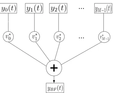
Classical BeamForming (BF), or spatial filtering, is an important research topic in array signal processing. It controls the weighting factors of all the sensors of the array to fix the array output in a desired direction. BF allows to estimate the DOA of source signal. The classical BF system can be seen in Fig. 2-2.

+

...

...

Fig. 2-2 Beamforming system

of the array. In order to estimate the DOA, the mth weighting coefficient is set as a function of

θ:

vm = ejωm. (2-5)

The output of the system can be written as

yBF(t) = M∑−1

m=0

v∗_mym(t). (2-6)

The power of the system output is

PBF(θ) = E[|yBF(t)|2]. (2-7)

The DOA estimation can be achieved by finding θ for the weighting coefficients v0, v1, . . . , vM−1

that can maximize the output power: ˆ

θ = max

θ PBF(θ). (2-8)

2.1.2.2 Linear Prediction (LP)

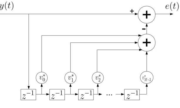
The LP estimator is a technique that can predict the unknown data with existing ones. Its system is shown in Fig. 2-3.

...

+

-+

+

Fig. 2-3 Linear prediction system

and y(t) is a weighted linear combination of the past data. Actually, LP estimation is a problem about searching the optimal weighting vector v = [v0, v1, . . . , vM−2]T so that

y(t) = M∑−2

m=0

y(t− m − 1)v∗_m. (2-9)

In 1967, Burg J. P. firstly proposed to use LP technique to estimate DOAs of far-field sources [56]. Let us look at Fig. 2-1. According to the LP technique, the received signal of the (M−1)th sensor can be predicted by those of the first M− 1 ones, y0(t), y1(t), . . . , yM−2(t), and it can be

expressed in the following matrix form:

yM−1(t) = [y0(t), y1(t), . . . , yM−2(t)][v0, v1, . . . , vM−2]H. (2-10)

By applying the conjugate operation, and premultiplying y_{lef t}(t) = [y0(t), y1(t), . . . , yM−2(t)]T,

we have

y_{lef t}y_M∗ ₋₁(t) = y_{lef t}(t)yH_{lef t}(t)v. (2-11) Take the expectation and the weighting vector can be obtained as

v = (E[y_{lef t}(t)yH_{lef t}(t)])−1E[y_{lef t}(t)y_M∗ (t)], (2-12) where E[·] denotes the ensemble average. The DOA estimation can be achieved with the fol-lowing spectrum: ˆ θk = arg max θ 1 aH_(θ)   −1 v     −1 v   H a(θ) , (2-13) where a(θ) = [1, ejω, ej2ω, . . . , ej(M−1)ω]T. (2-14) 2.1.2.3 MUSIC

The MUSIC algorithm was firstly proposed by Schmidt [16], which started the era of high resolution technique. Unlike LP, which directly process the covariance matrix of the received signal, MUSIC applies the EVD to the covariance matrix and gets its signal subspace and noise subspace. According to the orthogonality between these two subspaces, the MUSIC algorithm can successfully estimate the position parameters.

Let us assume that

The covariance matrix of y(t) is

R = E[y(t)yH(t)]

= A(θ)RsAH(θ) + σn2I, (2-16)

where

Rs = E[s(t)sH(t)], (2-17)

the kth column of A(θ) (also called steering vector) is

a(θk) = [1, ejωk, ej2ωk, . . . , ej(M−1)ωk]T, (2-18) σ2

n is the power of the spatially and temporally independent white Gaussian noise, and I is the

identity matrix. Applying the EVD to R leads to

RD = DΛ, (2-19)

where Λ is a diagonal matrix of eigenvalues arranging in decreasing order, and D the matrix formed by the corresponding eigenvectors:

Λ = diag(λ1, λ2, . . . , λK, λK+1, . . . , λM), (2-20)

D = [d1, d2, . . . , dK, dK+1, . . . dM]. (2-21)

We define the noise subspace as Uncontaining the M−K eigenvectors associated to the M −K

smallest eigenvalues: Un = [dK+1, . . . dM]. A(θ) is orthogonal with Unwhose proof is given

below.

Proof : Let us assume a situation without noise. Equation 2-16 can be written as

R0 = A(θ)RsAH(θ). (2-22)

The EVD of R0 is

R0D = DΛ. (2-23)

In Λ, there are K nonzero eigenvalues: λ1, λ2, . . . , λK, and λK+1 = . . . = λM = 0. According

to the definition of eigenvectors, R0dm = λmdm = 0 when K + 1 ≤ m ≤ M. Therefore,

A(θ) ⊥ Un.

When the additive white Gaussian noise is considered in the signal, the covariance matrix is written as

Let λ and d be a pair of eigenvalue and eigenvector of R0. Rd = (R0+ σ2nI)d

= R0d + σn2Id

= λd + σ_n2d

= (λ + σ_n2)d (2-25)

We can see that the additive white Gaussian noise only changes the eigenvalue. The eigenvectors of R0 are also the eigenvectors of R. Thus, the orthogonality between A(θ) and Unstill holds

when the white Gaussian noise exists and the estimation of DOA can be achieved through the following MUSIC spectrum

ˆ θk = arg max θ 1 aH_(θ)U nUHna(θ) . (2-26) 2.1.2.4 ESPRIT

ESPRIT is another subspace-based method. Unlike MUSIC, which is based on the orthogo-nality between the steering matrix and the noise subspace, it uses the signal subspace to estimate parameters. There is no requirement for spectrum search for ESPRIT, and the computational complexity is therefore reduced.

Firstly, we get the covariance matrix of the received signal from the array in Fig. 2-1:

R = E[y(t)yH(t)]

= A(θ)RsAH(θ) + σn2I, (2-27)

Apply the EVD to R, and we can get the signal subspace Us composed of the K eigenvectors

associated with the K biggest eigenvalues. The signal subspace Us can be divided into two

(M − 1) × K sub-matrices: Us=   Usup −   =   − Usdown   . (2-28)

Divide A(θ) into two (M − 1) × K parts:

A(θ) =   Aup(θ) −   =   − Adown(θ)   . (2-29)

[ejωk_{, e}j2ωk_{, . . . , e}j(M−2)ωk_{, e}j(M−1)ωk_]T _{respectively. We can easily observe that}

Adown(θ) = Aup(θ)Ω, (2-30)

where

Ω = diag{ejω1_{, . . . , e}jωK}. _(2-31)

There must be a non-singular matrix T that satisfies

Usup = Aup(θ)T, (2-32)

and

Usdown = Adown(θ)T. (2-33)

The diagonal matrix Ω contains the DOA information and therefore we can obtain the DOA by estimating Ω. By substituting Equation 2-30 and 2-32 into Equation 2-33, we have

Usdown = Adown(θ)T

= Aup(θ)ΩT

= UsupT−1ΩT. (2-34)

Apply the EVD to U♯_supUsdown (♯ denotes the pseudoinverse), and Ω can be estimated with the

eigenvalue matrix of U♯_supUsdown.

2.2

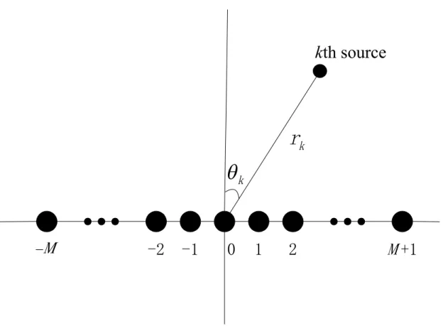
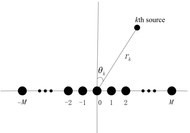
Near-field Source Model

As shown in Fig. 2-4, when sources are close to the array (i.e. in near-field situation), the plane wavefront assumption can no longer hold. In this case, the ranges of sources are supposed to be in the Fresnel region [0.62(R3_/ν)0.5_{, 2R}2_{/ν] with R being the aperture of the ULA [10, 57]}

and ν being the wavelength. The signal wavefront is spherical, and both the DOAs and ranges will be necessary to localize near-field sources. Consider K near-field narrow-band signals, impinging on the ULA. Suppose that the distance between two adjacent elements is d and there are 2M + 2 elements in the ULA, where M ≥ 1. Then the sampled baseband output of the mth sensor of the ULA can be written as

ym(t) =

K

∑

k=1

sk(t)ejφmk+ nm(t), t = 1, 2, . . . , T, (2-35)

where T is the number of samples, m ∈ [−M, M + 1], nm(t) is an additive Gaussian noise which may be coloured, sk(t) is the signal from the kth source and received by the 0th sensor,

-

-2

-1

0

1

2

+1

kth source

k



k

r

M

M

Fig. 2-4 Source localization in near-field with ULA

and φmk is the phase difference between the signals received at the mth sensor and 0th sensor,

due to the propagation of the signal from the kth source, given by

φmk = 2π ν ( √ r2 k+ (md)2− 2rkmd sin θk− rk), (2-36)

where θk represents the azimuth of the kth source and rk its range. The wavelength should

satisfy ν ≥ 4d [58]. By using the second-order Taylor expansion to (2-36), the phase difference

φmkcan be written as [59] φmk = (− 2πd ν sin θk)m + ( πd2 νrk cos2θk)m2+ o( d2 r2 k ) ≈ ωkm + ϕkm2, (2-37) with ωk =− 2πd ν sin θk, (2-38) and ϕk = πd2 νrk cos 2_θ k. (2-39)

The array output of (2-35) at time t could be expressed as          y_−M(t) y_−M+1(t) .. . yM +1(t)          =          ejφ−M1 _{. . . e}jφ_−MK ejφ(−M+1)1 _{. . . e}jφ(−M+1)K .. . . .. ... ejφ(M +1)1 _{. . . e}jφ(M +1)K                   s1(t) s2(t) .. . sK(t)          +          n_−M(t) n_−M+1(t) .. . nM +1(t)          (2-40) y(t) = A(θ, r)s(t) + n(t), (2-41)

where A(θ, r) is the steering matrix formed by steering vectors

a(θk, rk) = [ej(ωk(−M)+ϕk(−M)2)_{, . . . , e}j(ωk(M +1)+ϕk(M +1)2)_]T_{. (2-42)} s(t) and n(t) are the signal and noise vectors respectively:

s(t) = [s1(t), s2(t), . . . , sK(t)]T, (2-43)

n(t) = [n_−M(t), n_−M+1(t), . . . , nM +1(t)]T. (2-44)

The whole received signal matrix is

Y = A(θ, r)S + N, (2-45)

where

Y = [y(1), y(2), . . . , y(T )] (2-46)

S = [s(1), s(2), . . . , s(T )] (2-47)

N = [n(1), n(2), . . . , n(T )]. (2-48)

2.3

Second-order Statistics Methods

Second-order statistics are often used in traditional localization methods. The most signif-icant advantage is its low complexity. Based on second-order statistics, many researches have been carried out for near-field source localization, such as the 2D LP estimator [58], the 2D MUSIC method [23] and the modified 2D MUSIC algorithm [8].

2.3.1

2D LP Estimator

Based on the LP algorithm, Grosicki E. proposed a 2D LP estimator for near-field source localization [58]. Consider the array output in the near-field situation in Equation 2-35. Denote

r(p, q) the spatial correlation coefficient:

r(p, q) = E[yp(t)y∗q(t)]. (2-49)

Particularly, we have (for convenient illustration, assume that there is no noise)

r(−p, p) = K ∑ k=1 σ_sk2 e−2jpωk, (2-50) r(−p − 1, p) = K ∑ k=1 σ_sk2 e−j(ωk−ϕk)(2p+1), (2-51) r(−p + 1, p) = K ∑ k=1 σ_sk2 e−j(ωk+ϕk)(2p−1)_{. (2-52)}

There must be a unique (K + 1)-length vector vα = [vα(0), vα(1), . . . , vα(K)]T satisfying [60] K

∑

k=0

vα(k)r(−(p − k) + α, p − k) = 0. (2-53)

Then we have the roots of the polynomial f (z) = vα(0)zK+ vα(1)zK−1, . . . , vα(K):

zk= e−2jωk, α = 0 (2-54)

zk= e−2j(ωk−ϕk), α =−1 (2-55)

zk= e−2j(ωk+ϕk), α = 1 (2-56)

The DOA estimation can be achieved directly with ˆωkin Equation 2-54, but the range estimation

requires the correct paring of ωkand ϕk. We know that ωk = 1

2[(ωk+ ϕk) + (ωk− ϕk)]

ϕk =

1

2[(ωk+ ϕk)− (ωk− ϕk)]. The correct estimate of ϕkfor ˆωk is decided by

ˆ

ϕk =

1

with (p0, q0) given by (p0, q0) = arg min p,q |ˆωk− 1 2[(ωp+ ϕp) + (ωq− ϕq)]|. (2-58)

2.3.2

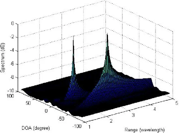
2D MUSIC

Due to the high resolution ability and estimation accuracy, MUSIC algorithm has attracted a lot of attention and become the most well-known algorithm of the spatial spectrum estimation theory. The earlier study of MUSIC mainly concentrated on DOA estimation for far-field source localization. However, as the localization of near-field sources grew more attractive, the demand for the estimation of multiple parameters was drawing attention from many researchers. How to adjust MUSIC algorithm to multiple parameter estimation became a hot topic. In [23, 61], 2D MUSIC method was proposed for near-field source localization. Like in the far-field situation, the joint range and DOA estimation can be achieved via the noise subspace.

Let us form the covariance matrix:

R = E[y(t)yH(t)]

= A(θ, r)RsAH(θ, r) + σn2I, (2-59)

Applying the EVD to R leads to

RD = DΛ, (2-60)

where Λ is a diagonal matrix of eigenvalues, and D the matrix formed by the corresponding eigenvectors:

Λ = diag(λ1, λ2, . . . , λK, λK+1, . . . , λ2M +2), (2-61)

D = [d1, d2, . . . , dK, dK+1, . . . d2M +2]. (2-62)

We define the noise subspace as Un containing 2M + 2 − K eigenvectors: Un =

[dK+1, . . . d2M +2]. Similar to the proof of the 1D MUSIC algorithm, we can also prove that A(θ, r) is orthogonal with Un.

The estimation of DOA and range can be gained through the following 2D MUSIC spec-trum (ˆθk, ˆrk) = arg max θ,r 1 aH_{(θ, r)U} nUHna(θ, r) . (2-63)

Fig. 2-5 2D MUSIC spectrum

two peaks which indicate the position of the two sources.

2D MUSIC maintains the high resolution and estimation accuracy. It can directly estimate the DOAs and ranges for all the near-field sources simultaneously without paring algorithms. However, as we can see from the figure, 2D MUSIC requires a 2D search for both the DOA and range.

2.3.3

Modified 2D MUSIC

To avoid the 2D search of near-field source localization, Jin He in [8] proposed to use the anti-diagonal information of the covariance matrix. The information is enough to form a Hermitian matrix for DOA estimation, but with the cost of aperture loss. This method can reduce the 2D search to K + 1 1D ones.

Jin He firstly calculated the covariance matrix R of the received signal from the first 2M +1 sensors. Then, he took the anti-diagonal elements to form a (2M + 1)× 1 vector as follows:

rx = [R(1, 2M + 1), R(2, 2M ), . . . , R(2M + 1, 1)]T (2-64)

where p_xis a K× 1 vector given by

p_x = [σ_s2₁, . . . , σ_sK2 ]T, (2-66) with σ2

sk being the power of the kth source, and

Ax(θ) = [ax(θ1), ax(θ2), . . . , ax(θK)], (2-67)

with ax(θk) being a (2M + 1)× 1 vector designed as follows:

ax(θk) = [ej2(−M)ωk, ej2(−M+1)ωk, . . . , ej2M ωk]T. (2-68)

He divided rx into G overlapping sub-vectors, with each sub-vector containing L elements

(2M + 1 = G + L− 1):

rxg = [rx(g), . . . , rx(g + L− 1)]T (2-69)

= AxL(θ)pxg, (2-70)

where g = 1, 2, . . . , G. The kth column of AxL(θ) is given by

axL(θk) = [e−j2ωk(M +1), e−j2ωkM, . . . , e−j2ωk(−M+G)]T, (2-71) and p_xg = [σ_s2₁ej2gω1_{, . . . , σ}2 sKe j2gωK ]T (2-72)

With a total of G groups, he computed the L× L covariance matrix of rxg as

Rx = 1 G G ∑ g=1 rxgrHxg. (2-73)

Apply the EVD to Rx and get the noise-subspace Unx. The DOA can be obtained from the

following 1D spectrum function: ˆ θk = arg max θ 1 aH xL(θ)UnxU H nxaxL(θ) . (2-74)

With the estimated DOA, the range estimation can be achieved by substituting each ˆθkinto the

following spectrum: ˆ rk= arg max r 1 aH_(ˆθ k, r)UnUHna(ˆθk, r) , (2-75)

where Unis the noise subspace obtained after applying the EVD to R. Unlike the DOA

esti-mation, this spectrum would yield only one peak, which represents the range estimate for the substituted kth DOA estimate ˆθk, reducing the 2D search to K + 1 1D ones.

However, Rx is of the size L× L. It is smaller than the size of the traditional covariance