Visiting Gafni's Reduction Land: from the BG Simulation to the Extended BG Simulation

HAL Id: inria-00389682

https://hal.inria.fr/inria-00389682

Submitted on 29 May 2009

HAL is a multi-disciplinary open access

archive for the deposit and dissemination of

sci-entific research documents, whether they are

pub-lished or not. The documents may come from

teaching and research institutions in France or

abroad, or from public or private research centers.

L’archive ouverte pluridisciplinaire HAL, est

destinée au dépôt et à la diffusion de documents

scientifiques de niveau recherche, publiés ou non,

émanant des établissements d’enseignement et de

recherche français ou étrangers, des laboratoires

publics ou privés.

Simulation to the Extended BG Simulation

Damien Imbs, Michel Raynal

To cite this version:

Damien Imbs, Michel Raynal. Visiting Gafni’s Reduction Land: from the BG Simulation to the

Extended BG Simulation. [Research Report] PI 1931, 2009, pp.12. �inria-00389682�

PI 1931 – mai 2009

Visiting Gafni’s Reduction Land:

from the BG Simulation to the Extended BG Simulation

Damien Imbs* , Michel Raynal**

damien.imbs@irisa.fr, raynal@irisa.fr

Abstract: The Borowsky-Gafni (BG) simulation algorithm is a powerful tool that allows a set of t + 1 asynchronous sequential processes to wait-free simulate (i.e., despite the crash of up to t of them) a large number n of processes under the assumption that at most t of these processes fail (i.e., the simulated algorithm is assumed to be t-resilient). The BG simulation has been used to prove solvability and unsolvability results for crash-prone asynchronous shared memory systems.

In its initial form, the BG simulation applies only to colorless decision tasks, i.e., tasks in which nothing prevents processes to decide the same value (e.g., consensus or k-set agreement tasks). Said in another way, it does not apply to decision problems such as renaming where no two processes are allowed to decide the same new name. Very recently (STOC 2009), Eli Gafni has presented an extended BG simulation algorithm (GeBG) that generalizes the basic BG algorithm by extending it to “colored” decision tasks such as renaming. His algorithm is based on a sequence of sub-protocols where a sub-protocol is either the base agreement protocol that is at the core of BG simulation, or a commit-adopt protocol.

This paper presents the core of an extended BG simulation algorithm that is particularly simple. This algorithm is based on two underlying objects: the base agreement object used in the BG simulation (as does GeBG), and (differently from GeBG) a new simple object that we call arbiter. As in GeBG, while each of the n simulated processes is simulated by each simulator, each of the first t + 1 simulated processes is associated with a predetermined simulator that we called its “owner”. The arbiter object is used to ensure that the permanent blocking (crash) of any of these t + 1 simulated processes can only be due to the crash of its owner simulator. After being presented in a modular way, the proposed extended BG simulation algorithm is proved correct.

Key-words: Arbiter, Asynchronous processes, Distributed computability, Fault-Tolerance, Process crash failure, Shared memory system, Wait-free environment, Reduction, t-Resilience.

De la BG Simulation `a la BG Simulation ´etendue

R´esum´e : Dans ce rapport, nous d´ecrivons comment passer de la BG simulation `a la BG simulation ´etendue.

Mots cl´es : Arbitre, Processus asynchrones, Calculabilit´e distribu´ee, Tol´erance aux fautes, Faute par crash, R´eduction, t-R´esilience, Syst`eme `a m´emoire partag´ee, Environnement sans attente.

*_{Projet ASAP: ´equipe commune avec l’INRIA, le CNRS, l’universit´e Rennes 1 et l’INSA de Rennes} **_{Projet ASAP: ´equipe commune avec l’INRIA, le CNRS, l’universit´e Rennes 1 et l’INSA de Rennes}

1

Introduction

What is the Boroswky-Gafni (BG) simulation Considering an asynchronous system where processes can crash, the (n, k)-set agree-ment problem is a basic decision task defined as follows [9]. Each of the n processes proposes a value, and every process that does not crash has to decide a value (termination), such that a decided value is a proposed value (validity) and at most k different values are decided (agreement). The consensus problem corresponds to the particular case k = 1.

A fundamental question related to distributed computability is the following. Suppose we have an algorithm that solves the (15, 4)-set agreement problem. Can we use this algorithm as a subroutine to solve the (12, 5)-4)-set agreement problem, assuming that at most t < 12 processes can crash? Intuitively, the answer might be “yes” (as we have less processes and more decided values are allowed). Let us now suppose that we want to use the same (15, 4)-set agreement subroutine to solve the (100, 4)-set agreement problem. As we have much more proposed values, and the same constraint on the number of decided values, an intuitive answer does not spring in an obvious way. And what is the answer if we want to solve the (80, 7)-set agreement problem (much more proposed values but only two more values can be decided), or (assuming t = 4) solve the (5, 4)-set agreement problem?

Stated in more general terms, the question is: “Can we use a solution to the (n, k)-set agreement problem as a subroutine to solve the (n0, k0)-set agreement problem, when at most t < min(n, n0) processes may crash?” (We say that “the (n0, k0)-set agreement is reducible to (n, k)-set agreement”.) The BG simulation (introduced in [6] and formalized and deeply investigated in [7] where is given a formal definition of “reducibility”) answers this fundamental question. It states that the answer if “yes” if k0 ≥ k and “no” if k0_{≤ t < k.} As we can see, the answer “yes” does not depend on the number of processes.

To that end, a BG simulation algorithm is described that allows n0 = t + 1 processes to simulate a large number n of processes that collectively solve a decision task in presence of at most t crashes. Each of the n0simulator processes simulates all the n processes. These n0simulator processes cooperate through underlying objects (the type of which is called here safe agreement) that allow them to agree on a single output for each of the non-deterministic statements issued by every simulated processes.

The important lesson learned from the BG simulation is that, in a failure-prone context, what is important is not the number of processes but the maximal number of possible failures and the actual number of values that are proposed to a decision task. An interesting application of the BG simulation (among several of its applications [7]) is the proof that there is no t-resilient (n, k)-set agreement algorithm for t ≥ k. This is obtained as follows. As (1) the BG simulation allows reducing the (k + 1, k)-set agreement problem to the (n, k)-set agreement problem in a system with up to k failures, and (2) the (k + 1, k)-set agreement problem is known to be impossible in presence of k failures [6, 13, 16], it follows that there is no k-resilient (n, k)-set agreement algorithm.

The limit of the BG-simulation and the extended BG-simulation The BG simulation characterizes t-resilient solvability by reducing it to the question of wait-free solvability (i.e., t-resilience in a system of n = t + 1 processes). Unfortunately, the BG simulation is limited to colorless decision tasks, i.e., tasks in which if a process decides a value v, then all the processes can decide that value (the class of colorless tasks is formally defined in [7]). The (n, k)-set decision problem is typically such a task. From an operational point of view, this is due to the fact that, in the BG simulation, each simulator simulates fairly all the processes, and consequently, the crash of a simulator process can manifest itself as the crash of any simulated process (the one it is currently simulating a critical part of code).

The extended BG simulation has been proposed by Eli Gafni to overcome this limitation and consequently fully capture t-resilience [12]. As stated in [12] “With the extended BG simulation we can reduce questions about t-resilience solvability to questions about wait-free solvability. The latter is characterized by the Herlihy-Shavit conditions [13]”.

As a result, it applies to both colorless tasks and colored decision tasks such as the renaming problem [3]. In that problem, each of the n processes has to decide a new name (from a given new name space) such that no two processes have the same new name. This problem has wait-free solutions when the new name space [1..M ] is such that M ≥ 2n − 1 (see [8] for a deeper insight into the problem).

In his paper [12], Gafni presents several (un)decidability results that can be obtained in a simpler way from the BG simulation. He also uses the extended BG simulation to show that the t-resilient weak symmetry breaking problem is equivalent to t-resilient weak renaming problem.

The core of the BG simulation relies on the following principles: (1) each of the (t + 1) simulators fairly simulates all the processes, and this simulation is such that (2) the crash of a simulator entails the crash of at most one simulated process. The BG simulation is “symmetric” in the sense that each of the n processes is simulated by every simulator, and the (t + 1) simulators are “equal” with respect to each simulated process. One way to be able to simulate colored tasks (without preventing the simulation of colorless tasks), consists in introducing some form of asymmetry [12].

The extended BG simulation realizes the appropriate asymmetry as follows. As in th BG simulation each simulator process q simulates all the processes, but it is associated with a given simulated process p (in our terminology, q is the owner of p). Then ownership notion is used to to ensure that the corresponding simulated process p will not be blocked forever (perceived as crashed) if its owner simulator q does not crash. Hence, if a simulator does not crash, it can always decide the value decided by the simulated process

p it “owns”. As noticed and demonstrated in [12] “extending the BG simulation by this simple property results in a full characterization of t-resilience in terms of wait-freedom”.

Content of the paper In addition to the introduction of the notion of extended BG simulation, and a full characterization of t-resilience, Gafni presents in [12] an extended BG simulation algorithm (denoted here GeBG). This algorithm is based on a sequence of sub-protocols where each sub-protocol is either the base agreement protocol used in the BG simulation (safe agreement type objects) or a commit-adopt protocol [11]. This algorithm is presented informally in English.

The present paper presents the core of an extended BG simulation algorithm that is particularly simple. This algorithm is based on two underlying object types: the type safe agreement (the one used in the BG simulation algorithm and in GeBG), and (differently from GeBG) an object type that we call arbiter. An arbiter object allows exploiting the ownership notion in a simple way to ensure that (1) an object value is always decided when its owner does not crash, and (2) the value of that object is determined either by its owner simulator or by the other simulators.

As far as the whole simulation is concerned, while (as in the BG simulation) each of the n simulated processes is simulated by each simulator, (as in GeBG) each of the first t + 1 simulated processes is “associated” with exactly one simulator (its “owner”). As already said, it follows from the appropriate use of the arbiter objects that the permanent blocking (crash) of any of these t + 1 simulated processes can only be due to the crash of its owner simulator.

The paper is made up of 7 sections. Section 2 presents the model and the definition of decision tasks. Section 3 explains the structure of the simulation. Section 4 defines the base object types used by the simulators to cooperate and realize a correct simulation. Then, the extended BG simulation algorithm is presented in an incremental and modular way. First Section 5 briefly presents the BG simulation algorithm, and then Section 6 enriches it to solve the extended BG simulation. This algorithm is proved in Section 7.

2

Solving decision tasks

2.1

Decision tasks

The problems we are interested in are called decision tasks1_{. In every run, each process proposes a value and the proposed values define} an input vector I where I[j] is the value proposed by pj. Let I denote the set of allowed input vectors. Each process has to decide a value. The decided values define an output vector O, such that O[j] is the value decided by pj. Let O be the set of the output vectors.

A decision task is a binary relation ∆ from I into O. A task is colorless if, when a value v is decided by a process pj(i.e., O[j] = v), then v can be decided by all the processes). Consensus, and more generally k-set agreement, are colorless tasks. Otherwise the task is colored. Renaming is a colored task.

2.2

The computation model

Asynchronous processes and fault model We are interested in distributed algorithms the aim of which is to solve a task in a system made up of n asynchronous sequential processes denoted p1, ..., pn. A process executes a sequence of atomic steps (as defined by its algorithm). Each process pjis endowed with a write-once local variable outputjwhere it deposits the value it decides.

A process can crash in a run. A process executes correctly the steps defined by its algorithm until it crashes (if ever it does). After if has crashed, a process executes no more steps. If it does not crash, a process executes an infinite number of steps.

It is assumed that an arbitrary subset (not known in advance) of up to t < n processes can crash (the crash of one process being independent from the crash of other processes). A process that does not crash in a run is said to be correct in that run, otherwise it is faulty. This failure model is called the t-resilient environment, and an algorithm designed for such an environment is said to be t-resilient. The extreme case t = n − 1 is called wait-free environment, and the corresponding algorithms are called wait-free algorithms.

Communication model The n processes cooperate through a shared memory made up of a snapshot object [1] denoted mem. This means that a process pj can write only the entry mem[j] but can read all the entries by invoking the operation mem.snapshot(). The write and snapshot operation appears as being executed atomically [1]. (These operations can be built on top of a single-writer/multiple-readers atomic registers [1, 4]). Initially, mem[j] = ⊥.

Definition The previous computation model (asynchronous crash-prone processes that communicate through snapshot objects) is called snapshot model.

2.3

Algorithm solving a task

An algorithm solves a task in a t-resilient environment if, given any I ∈ I, each correct process pj decides (i.e., writes a value v in outputj) and there is an output vector O such that (I, O) ∈ ∆ where O is defined as follows. If pjdecides v, then O[j] = v. If pjdoes not decide, O[j] is set to any value v0that preserves the relation (I, O) ∈ ∆.

A task is solvable in a t-resilient environment if there is an algorithm that solves it in that environment. As an example, consensus is not solvable in the 1-resilient environment [10, 14, 15]. Differently, renaming with 2n−1 names is solvable in the wait-free environment [5, 3, 13].

3

Simulated processes vs simulator processes

Aim Let A be an n-process t-resilient algorithm that solves a decision task in the base snapshot model described previously. The aim is to design a (t + 1)-process wait-free algorithm A0 that simulates A in the same snapshot model. (The reader is referred to [7] for a formal definition of a simulation.)

Notation A simulated process is denoted pj with 1 ≤ j ≤ n, and the subscript j is always used to refer to a simulated process. Similarly, a simulator process (in short “simulator”) is denoted qi with 1 ≤ i ≤ t + 1, and the subscript i is always used to refer to a simulator.

As far the objects accessed by the simulators are concerned, the following convention is adopted. The objects denoted with upper case letters are the objects shared by the simulators. Differently an object denoted with lower case letters is local to a simulator (in that case, the associated subscript denotes the corresponding simulator).

What does a simulator Each simulator qiis given the code of all the simulated processes p1, . . . , pn. It manages n threads, each one associated with a simulated process, and locally executes these threads in a fair way. It also manages a local copy memiof the snapshot memory mem shared by the simulated processes.

The code of a simulated process pjcontains writes of mem[j] and invocations of mem.snapshot(). These are the only operations used by the processes p1, . . . , pn to cooperate. So, the core of the simulation is the definition of two algorithms. The first (denoted sim writei,j()) has to describe what a simulator qihas to do in order to correctly simulate a write of mem[j] issued by a process pj. The second (denoted sim sanpshoti,j()) has to describe what a simulator qi has to do in order to correctly simulate an invocation of mem.sanpshot() issued by a process pj.

4

Base object types used in the simulation

In addition to snapshot objects, the simulator processes cooperate through atomic read/write register objects, and specific objects the types of which (safe agreement and arbiter) are defined in this section. These types can be implemented from multi-reader/multi-writer atomic registers, which in turn can be implemented from snapshot objects. Hence, all the base objects used in the simulation can be implemented in the snapshot computation model described in the previous section.

4.1

The safe agreement object type

The safe agreement type This object type (defined in [6, 7]) is at the core of the BG simulation. It provides each simulator qi with two operations, denoted propose_i(v) and decidei(), that qican invoke at most once, and in that order. The operation proposei(v) allows qi to propose a value v while decidei() allows it to decide a value. The properties satisfied by an object of the type safe agreement, owned by qj, are the following.

• Termination. If no simulator qxcrashes while executing proposex(), then any correct simulator qithat invokes decidei(), returns from that invocation.

• Agreement. At most one value is decided. • Validity. A decided value is a proposed value.

init: for each x : 1 ≤ x ≤ t + 1 do SM [x] ← (⊥, 0) end for. operation proposei(v): % 1 ≤ i ≤ t + 1 %

(01) SM [i] ← (v, 1); (02) smi← SM.snapshot();

(03) if (∃x : smi[x].level = 2) then SM [i] ← (v, 0) else SM [i] ← (v, 2) end if.

operation decidei(): % 1 ≤ i ≤ t + 1 %

(04) repeat smi← SM.snapshot() until (∀x : smi[x].level 6= 1) end repeat;

(05) let x = min({k | smi[k].level = 2); res ← smi[x].value;

(06) return(res).

Figure 1: An implementation of the safe agreement type [7] (code for qi)

An implementation The implementation of the safe agreement type described in Figure 1 is from [7]. This construction is based on a snapshot object SM (with one entry per simulator qi). Each entry SM [i] of the snapshot object has two fields: SM [i].value that contains a value and SM [i].level that stores its level. The level 0 means the corresponding value is meaningless, 1 means it is unstable, while 2 means it is stable.

When a simulator qi invokes proposei(v), it first writes the pair (v, 1) in SM [i] (line 01), and then reads the snapshot object SM (line 02). If there is a stable value in SM , pi“cancels” the value it proposes, otherwise it makes it stable (line 03).

A simulator qiinvokes decidei() after it has invoked proposei(). Its aim is to return the same stable value to all the simulators that invoke this operation (line 06). To that end, qirepeatedly computes a snapshot of SM until it sees no unstable value in SM (line 04). Let us observe that, as a simulator qiinvokes decidei() after it has invoked proposei(v), there is at least one stable value in SM when it executes line 05. Finally, in order that the same stable value be returned to all, qireturns the stable value proposed by the simulator with the smallest id (line 05).

A formal proof that this algorithm implements the safe agreement type is given [7]. For completeness purpose, a proof is also given in Appendix A.

4.2

The arbiter object type

Definition Similarly to the objects of type safe agreement, each object of the type arbiter has a statically predefined owner simulator qj. Such an object provides the simulators with a single operation denoted arbitratei,j() (where i is the id of the invoking simulator and j the id of the owner). A simulator qiinvokes arbitratei,j() at most once, and, when it terminates, this invocation returns a value to qi. The properties of an object of the type arbiter owned by qjare the following.

• Termination. If the owner qjinvokes arbitratej,j() and is correct, or does not invoke arbitratej,j(), or if a simulator qiterminates its invocation arbitratei,j(), then all the correct simulators returns from their arbitratei,j() invocation.

• Agreement. No two processes return different values.

• Validity. The returned value is 1 (owner) or 0 (not owner). Moreover, if the owner does not invoke arbitratej,j(), 1 cannot be returned, and if only the owner invokes arbitratei,j(), 0 cannot be returned.

An implementation An implementation of an object of the type arbiter is described in Figure 2. It is based on a snapshot object PART (initialized to [false, . . . , false]), and an atomic register WINNER (initialized to ⊥).

When it invokes arbitratei,j(), the simulator qiannounces that it participates (line 01), and issues a snapshot to know the simulators that are currently participating (line 02). If qiis the owner of the object (i = j, line 03), it checks if it is the first participant (predicate parti = {i}). If it is, it sets WINNER to 1, otherwise it sets it to 0 (line 04). If piis not the owner of the object (i 6= j), it checks if the owner is a participating simulator (predicate j ∈ parti). If is its, qiwaits to know which value has been assigned to WINNER. If it is not, it sets WINNER to 0. Finally, qiterminates by returning the value of WINNER.

operation arbitratei,j(): % 1 ≤ i, j ≤ t + 1 %

(01) PART [i] ← true;

(02) auxi← PART .snapshot(); parti← {x | auxi[x]};

(03) if (i = j) % piis the owner of the associated arbiter type object %

(04) then if (part_i= {i}) then WINNER ← 1 else WINNER ← 0 end if (05) else if (j ∈ parti) then wait (WINNER 6= ⊥) else WINNER ← 0 end if

(06) end if;

(07) return(WINNER).

A proof that this construction implements the arbiter object type is given in Appendix B.

5

The BG simulation

This section presents the BG simulation [6, 7]: its main principles and the algorithms implementing its base operations sim writei,j() and sim snapshot_i,j().

5.1

The shared memory MEM [1..(t + 1)]

The snapshot memory mem shared by the processes p1, . . . , pnis emulated by a snapshot object MEM shared by the simulators (so, MEM has (t + 1) entries).

More specifically, MEM [i] is an atomic register that contains an array with one entry per simulated process pj. Each MEM [i][j] is made up of two fields: MEM [i][j].value that contains the last value of mem[j] written by pj, and MEM [i][j].sn that contains the associated sequence number. (This sequence number, introduced by the simulation, is a control data that will be used to produce a consistent simulation of the mem.snapshot() operations issued by the simulated processes pj).

5.2

The sim write

() operation

The algorithm, denoted sim writei,j(v), executed by qito simulate the write by pjof the value v into mem[j] is described in Figure 3 [7]. Its code is pretty simple. The simulator qifirst increases a local sequence number w sni[j] that will be associated with the value v written by pjinto mem[j]. Then, qiwrites the pair (v, w sni[j]) into memi[j] (where memiis its local copy of the memory shared by the simulated processes) and finally writes atomically its local copy memiinto MEM [i].

operation sim writei,j(v):

(01) w sni[j] ← w sni[j] + 1;

(02) memi[j] ← (v, w sni[j]);

(03) MEM [i] ← memi.

Figure 3: writei,j(v) executed by qito simulate write(v) issued by pj(from [7])

5.3

The sim snapshot

() operation

This operation is implemented by the algorithm described in Figure 4 [7].

Additional local and shared objects For each process pj, a simulator qimanages a local sequence number generator snap sni[j] used to associates a sequence number with each mem.snapshot() it simulates on behalf of pj(line 04).

In addition to the snapshot object MEM [1..(t + 1)], the simulators q1, . . . , qt+1cooperate through an array SAFE AG[1..n, 0...] of safe agreement type objects.

Underlying principle of the BG simulation [6, 7]: obtaining a consistent value In order to agree on the very same output of the snapsn-th invocation of mem.snapshot() that is issued by pj, the simulators q1, . . . , qt+1use the object SAFE AG[j, snapsn].

Each simulator qi proposes a value (denoted inputi) to that object (line 05) and, due to its agreement property, that object will deliver them the same output at line 06. In order to ensure the consistent progress of the simulation, the input value inputiproposed by the simulator qito SAFE AG[j, snapsn] is defined as follows.

• First, qiissues a snapshot of MEM in order to obtain a consistent view of the simulation state. The value of this snapshot is kept in smi(line 01).

Let us observe that smi[x][y] is such that (1) smi[x][y].sn is the number of writes issues by py into mem[y] that have been simulated up to now by qx, and (2) smi[x][y].value is the value of the last write into mem[y] as simulated by qxon behalf of py. • Then, for each py, qi computes inputi[y]. To that end, it extracts from smi[1..t + 1][y] the value written by the more advanced

simulator qsas far as the simulation of pyis concerned. This is expressed in lines 02-03.

Once, inputihas been computed, qiproposes it to SAFE AG[j, snapsn] (line 05), and then returns the value decided by that object (lines 06-07).

The previous description shows an important feature of the BG simulation. A value inputi[y] = smi[s][y].value proposed by a simulator qi can be such that smi[s][y].sn > smi[i][y].sn, i.e., the simulator qsis more advanced than qias far as the simulation of

operation sim snapshoti,j():

(01) smi← MEM .snapshot():

(02) for each y : 1 ≤ y ≤ n: do inputi[y] = smi[s][y].value

(03) where ∀x : 1 ≤ x ≤ t + 1 : smi[s][y].sn ≥ smi[x][y].sn end for;

(04) snap sni[j] ← snap sni[j] + 1; let snapsn = snap sni[j];

(05) enter mutex; SAFE AG[j, snapsn].proposei(inputi); exit mutex;

(06) res ← SAFE AG[j, snapsn].decidei()

(07) return(res).

Figure 4: sim snapshoti,j() executed by qito simulate mem.snapshot() issued by pj(from [7])

py is concerned. This causes no problem, as when qiwill simulate mem.snapshot() operations for py (if any) that are between the (smi[i][y].sn)-th and the (smi[s][y].sn)-th write operations of py, it will obtain a value that has already been computed and is currently kept in the corresponding SAFE AG[y, −] object.

Underlying principle of the BG simulation [6, 7]: from wait-freedom to t-resilience Each simulator qi simulates the n pro-cesses p1, . . . , pn “in parallel” and in a fair way. But any qi can crash. The crash of qi while it is engaged in the simulation of mem.snapshot() on behalf of several processes pj, pj0, etc., can entail their definitive blocking, i.e., their crash. This is because

each SAFE AG[j, −] object guarantees that its SAFE AG[j, −].decide() invocations do terminate only if no simulator crashes while executing SAFE AG[j, −].propose() (line 05 of Figure 4).

The simple (and bright) idea of the BG simulation to solve this problem consists in allowing a simulator to be engaged in only one SAFE AG[−, −].propose() invocation at a time. Hence, if qi crashes while executing SAFE AG[j, −].propose(), it can entails the crash of pj only. This is obtained by using an additional mutual exclusion object offering the operations enter mutex and exit mutex. (Let us notice that such a mutex object is purely local to each simulator: it solves conflicts among the simulating threads inside each simulator, and has nothing to do with the memory shared by the simulators).

From t-resilience to wait-freedom As an example let us consider we have a t-resilient agorithm that solves the (n, t) agreement problem. We obtain a wait-free algorithm that solves the (t + 1, t) agreement problem as follows. Each simulator qi (1 ≤ i ≤ t + 1) is initially given a proposed value vi, and the base objects SAFE AG[1..n, 0] are used by the (t + 1) simulators as follows to determine the value proposed by pj. For each j, 1 ≤ j ≤ n, the simulator qi invokes first SAFE AG[j, 0].proposei(vi) and then SAFE AG[j, 0].decidei() that returns it a value that it considers as the value proposed by pj. It is easy to see that, for any j, all the simulators obtain the same value for pj. Moreover, this value is one of the t + 1 values proposed by the simulators. Finally, simulator process qi can decide any of the values decided by the processes pj it is simulating. (It is easy to see that the BG simulation is for colorless decision tasks.) A formal proof of this reduction (based on input/output automata) can be found in [7].

From wait-freedom to t-resilience For colorless decision tasks, t-resilience can easily be reduced to wait-freedom as follows. First, each application process deposits its input value in a shared register. Then, every process of the t + 1 processes of the wait-free algorithm takes one of those values as its input value and executes its code. Finally, each application process decides any value decided by a process of the wait-free algorithm.

6

The extended BG simulation

This section extends the previous algorithms in order to solve the extended BG simulation. Our aim is to obtain an implementation hat is “as simple as possible”. To that end, we proceed incrementally by “only” enriching the previous base BG simulation. The proposed implementation uses the same snapshot object MEM and the same sim writei,j() operation (Figure 3) as the base BG simulation. It also uses the same SAFE AG[1..n, 0...] array made up of safe agreement type objects.

This section presents the additional shared objects that are used, the underlying principles on which relies the implementation of mem.snaspshot() issued by a simulator qi on behalf of a simulated process pj, and the algorithm (denoted e sim snapshoti,j()) that implements it.

6.1

The additional shared objects

In addition to MEM and SAFE AG[1..n, 0...], the memory shared by the simulators q1, . . . , qt+1contains the following objects. • ARBIT ER[1..t + 1, 0...] is an array of arbiter objects. The objects ARBIT ER[j, −] are owned by the simulator qj (1 ≤ j ≤

The object ARBIT ER[j, snapsn] is used by a simulator qi when it simulates its snapsn-th invocation mem.snapshot() on behalf of the simulated process pj for 1 ≤ j ≤ t + 1. (As we will see, when t + 1 < j ≤ n, the simulation of mem.snapshot() on behalf of pjdoes not require the help of an arbiter object.)

• ARB VAL[1..t + 1, 0...][0..1] is an array of pairs of atomic registers. The pair of atomic registers ARB VAL[j, snapsn][0..1] is used in conjunction with the arbiter object ARBIT ER[j, snapsn].

The aim of ARB VAL[j, snapsn][1] is to contain the value that has to be returned to the snapsn-th invocation mem.snapshot(), on behalf of the simulated process pj, if the owner qjis designated as the winner by the associated ARBIT ER[j, snapsn] object. If the owner qjis not the winner, the value that has to be returned is the one kept in ARB VAL[[j, snapsn][0].

6.2

The e sim snapshot

() operation

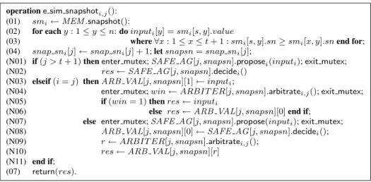
The enriched algorithm The code of the algorithm that implements the operation e sim snapshoti,j() executed by qi to simulate a mem.snapshot() operation issued by pjis described in Figure 5. Its first four lines and its last line are exactly the same as in Figure 4. The lines 05-06 are replaced by the new lines N01-N11 that constitutes the “addition” that allows going from the BG to the extended BG simulation.

Underlying principle Albeit each simulated process pj (1 ≤ j ≤ n) is simulated by each simulator qi(1 ≤ i ≤ t + 1) as in the BG simulation, each simulated process pj such that 1 ≤ j ≤ t + 1 is associated with exactly one simulator that is its “owner”: qi is the owner of pjif j = i (and also the owner of the corresponding objects ARBIT ER[j, −]). The aim is, for any snapsn ≥ 0, to associate a single returned value with the snapsn-th invocations of e sim snapshot_i,j() issued by the simulators. The idea is to use the ownership notion to “shortcut” the use of SAFE AG[j, snapsn] object in appropriate circumstances.

The operation e sim snapshot_i,j() for the simulated processes pjsuch that t + 2 ≤ j ≤ n, is exactly the same as sim snapshoti,j(). This appears in the lines N01-N02 that are the same as the lines 06-07 of Figure 4 (in that case, there is no ownership notion and consequently no simulator qiever invokes SAFE AG[j, snapsn].abortj()).

The new lines N03-N10 address the case of the simulated processes owned by a simulator, i.e., the processes p1, . . . , pt+1. The idea is the following: if qidoes not crash, pi has not to crash. In that way, if qiis correct, pi will always terminate whatever the behavior of the other simulators. To that end, qi on one side, and all the other simulators on the other side, compete to define the snapshot value returned by the snapsn-th invocations e sim snapshoti,j() issued by each of them. To attain this goal, the additional objects ARBIT ER[j, snapsn] and ARB VAL[j, snapsn] are used in the following way.

All the simulators invoke ARBIT ER[j, snapsn].arbitratei,j() (at line N04 if qiis the owner, and line N09 if it is not). According to the specification of the arbiter type, these invocations do not return different values, and do return at least when the owner qjis correct and invokes that operation (as indicated in the specification, there are other cases where the invocations do terminate). Finally, the value returned indicates if the winner is the owner (1) or not (0).

If the winner is the owner qj, the value returned by the snapsn-th invocations of e sim snapshoti,j() (one invocation by simulator) is the value inputjcomputed by the owner. That value is kept in the atomic register ARB VAL[j, snapsn][1] (line N03).

If the owner is not the winner, the value returned is the value determined by the other (non-owner) simulators that have invoked SAFE AG[j, snapsn].propose_i(inputi) (line N07) and SAFE AG[j, snapsn].decidei() (line N09). The value they have computed has been deposited in ARB VAL[j, snapsn][0] (line N08), and is used as the result of the SAFE AG[j, snapsn] object.

It is important to notice that the owner qjdoes not invoke proposej() and decidej() on the objects it owns. Moreover, the simulator qjis the only that can write ARB VAL[j, snapsn][1], while the other simulators can write only ARB VAL[j, snapsn][0].

To summarize, if a simulator qi crashes, it entails the crash of at most one simulated process. This is ensured thanks to the mutex algorithm. If the simulator qicrashes, 1 ≤ i ≤ t + 1, as far the simulated processes are concerned, it can entail either no crash at all (if qicrashes outside a critical section), or the crash of pi(if it crashes while executing arbitratei,j() inside the critical section at line N04), or the crash of a process pjsuch that 1 ≤ j 6= i ≤ t + 1 (this can occur only if qjhas crashed and was not winner, and qicrashes inside the critical section at line N08), or the crash of one of the processes pt+2, ..., pn(if it crashes at line N01 inside the critical section). t-Resilience vs wait-freedom Given a BG simulation algorithm where a simulated process pj(1 ≤ j ≤ t + 1 ≤ n) can be blocked forever only if the simulator qj crashes, Gafni shows in [12] that wait-freedom and t-resilience are equivalent for decision tasks (this paper shows also strong results on equivalence between weak renaming and weak symmetry breaking).

7

Proof of the extended BG simulation

operation e sim snapshoti,j():

(01) smi← MEM .snapshot():

(02) for each y : 1 ≤ y ≤ n: do inputi[y] = smi[s, y].value

(03) where ∀x : 1 ≤ x ≤ t + 1 : smi[s, y].sn ≥ smi[x, y].sn end for;

(04) snap sni[j] ← snap sni[j] + 1; let snapsn = snap sni[j];

(N01) if (j > t + 1) then enter mutex; SAFE AG[j, snapsn].proposei(inputi); exit mutex;

(N02) res ← SAFE AG[j, snapsn].decidei()

(N03) elseif (i = j) then ARB VAL[j, snapsn][1] ← inputi;

(N04) enter mutex; win ← ARBIT ER[j, snapsn].arbitratei,j(); exit mutex;

(N05) if (win = 1) then res ← inputi

(N06) else res ← ARB VAL[j, snapsn][0] end if;

(N07) else enter mutex; SAFE AG[j, snapsn].propose(inputi); exit mutex;

(N08) ARB VAL[j, snapsn][0] ← SAFE AG[j, snapsn].decidei();

(N09) r ← ARBIT ER[j, snapsn].arbitratei,j();

(N10) res ← ARB VAL[j, snapsn][r]

(N11) end if; (07) return(res).

Figure 5: The operation e sim snapshot_i,j() executed by qito simulate mem.snapshot() issued by pj

Proof A simulator can block the simulation of a process only during an e sim snapshot() operation, when the simulator uses a safe agreement (lines N01-N02 or N07-N08) or an arbiter object because it is its owner (line N04). All these invocations are placed in mutual exclusion. Thus a simulator can block the simulation of only a single process at a time. 2Lemma 1

Lemma 2 The simulated process piis never blocked at the simulatorqi.

Proof The e sim snapshot() operation, when invoked by simulator qifor the simulated process pi(line N03, i = j) does not include any wait statement and does not use a safe agreement object. Due to the properties of the arbiter object type, it cannot be blocked during its invocation of arbitrate(). Thus, the simulated process pican never be blocked at simulator qi. 2Lemma 2

Lemma 3 Each simulator receives the decision value of at least n − t simulated processes.

Proof Because at most t simulators may crash, and a simulator can block at most a single simulated process at a time (Lemma 1), each simulator can execute the code of at least n − t simulated processes without being blocked forever. Because the simulated algorithm is t-resilient, these n − t processes will then decide a value. 2Lemma 3 Lemma 4 All simulators that return a value for the k-th snapshot of the simulated process pjreturn the same value.

Proof If the simulated process qj isn’t owned by any simulator (j > t + 1), then because of the properties of the safe agreement objects, the same snapshot is always returned (lines N01-N02 of Figure 5).

If the owner of the simulated process pj chooses the value it has computed for pj’s k-th snapshot, it has written this value in ARB V AL[j, snapsn][1] (line N03), and is the winner of the arbiter object (line N05). All other simulators will then read its value (line N10).

If the simulated process has an owner but another process chooses the value it has computed for pj’s k-th snapshot, this process has already agreed on a value with all other non owner processes (safe agreement object, lines N07-N08) and is the winner of the arbiter object (lines N09-N10). All non-owner processes will then write the same value in ARB V AL[j, snapsn][0] (line N08) and the owner will read it (line N06).

Thus, all simulators that return a value for the k-th snapshot of the simulated process pjreturn the same value. 2Lemma 4

Lemma 5 At most one decision value can be decided by a simulated process on any simulator.

Proof Because every simulator computes the same value for any given snapshot and because the snapshot operations are the only non-deterministic parts of codes of the simulated processes, all simulators that decide a value for a given simulated process decide the

same value. 2Lemma 5

Lemma 6 The sequences of all writes and snapshots for each simulated process correspond to a correct execution of the simulated algorithm.

Proof Every simulator that is not blocked while simulating a process simulates it in the same way (same values written and same snapshots read, Lemma 4).

When simulator qi executes e sim snapshot() for pj (i.e. the simulation of a snapshot for pj), it stores in its inputi variable the values written by the simulators that have advanced the most for each simulated process (Figure 3 and lines 01-03 of Figure 5). It can choose its own input_i snapshot value only if no other simulator has already ended the execution of this e sim snapshot() (Lemma 4 implies that safe agreement objects have a “memory” effect). Thus, for each e sim snapshot(), qireturns an input value computed by itself or another simulator. Let us notice that, when this input value has been determined, no simulator had terminated its associated e sim snapshot(). (If this was not the case, that simulator would have provided the other simulators with its own input value.) Because processes are simulated deterministically, the input value returned contains the last value written by pj as seen by qi. This shows that the simulated process order is respected.

To ensure that the simulation is correct, we then have to show that the writes and snapshots of all processes can be linearized. The linearization point of the writes is placed at line 03 of Figure 3 of the first simulator that executes it. The linearization point of the snapshots is placed at line 01 of Figure 5 of the simulator qithat imposes its inputivalue.

Because the simulator qithat imposes its inputivalue in a e sim snapshot() operation reads the most advanced values at the time of its snapshot (lines 02-03 of Figure 5), and because once a simulator finishes the execution of e sim snapshot(), the value for this e sim snapshot() cannot change (Lemma 4), the linearization correspond to a linearization of a correct execution of the simulated

algorithm. 2Lemma 6

Theorem 1 The extended BG simulation algorithms described in Figures 3 and 5 are correct.

Proof Lemmas 2, 3, 5 and 6 show that the extended BG simulation algorithms presented here are correct. 2T heorem 1

Acknowledgments

The authors want to acknowledge E. Gafni, S. Rajsbaum, and C. Travers for interesting discussions on the BG-simulation.

References

[1] Afek Y., Attiya H., Dolev D., Gafni E., Merritt M. and Shavit N., Atomic Snapshots of Shared Memory. Journal of the ACM, 40(4):873-890, 1993.

[2] Afek Y., Gafni E., Rajsbaum S., Raynal M. and Travers C., Simultaneous consensus tasks: a tighter characterization of set consensus. Proc. 8th Int’l Conference on Distributed Computing and Networking (ICDCN’06), Springer Verlag LNCS #4308, pp. 331-341, 2006.

[3] Attiya H., Bar-Noy A., Dolev D., Peleg D. and Reischuk R., Renaming in an Asynchronous Environment. Journal of the ACM, 37(3):524-548, 1990. [4] Attiya H. and Rachman O., Atomic Snapshots in O(n log n) Operations. SIAM Journal on Computing, 27(2):319-340, 1998.

[5] Attiya H. and Welch J., Distributed Computing, Fundamentals, Simulation and Advanced Topics (Second edition). Wiley Series on Parallel and Distributed Computing, 414 pages, 2004.

[6] Borowsky E. and Gafni E., Generalized FLP Impossibility Results for t-Resilient Asynchronous Computations. Proc. 25th ACM Symposium on Theory of Com-puting (STOC’93), ACM Press, pp. 91-100, 1993.

[7] Borowsky E., Gafni E., Lynch N. and Rajsbaum S., The BG distributed simulation algorithm. Distributed Computing, 14(3):127-146, 2001.

[8] Casta˜neda A. and Rajsbaum S., New Combinatorial Topology Upper and Lower Bounds for Renaming. Proc. 27th ACM Symposium on Principles of Distributed Computing (PODC’08), ACM Press, pp. 295-304, Toronto (Canada), 2008.

[9] Chaudhuri S., More Choices Allow More Faults: Set Consensus Problems in Totally Asynchronous Systems. Information and Computation, 105:132-158, 1993. [10] Fischer M.J., Lynch N.A. and Paterson M.S., Impossibility of Distributed Consensus with One Faulty Process. Journal of the ACM, 32(2):374-382, 1985. [11] Gafni E., Round-by-round Fault Detectors: Unifying Synchrony and Asynchrony. Proc. 17th ACM Symposium on Principles of Distributed Computing (PODC’98),

ACM Press, pp. 143-152, 1998.

[12] Gafni E., The Extended BG Simulation and the Characterization of t-Resiliency. Proc. 41th ACM Symposium on Theory of Computing (STOC’09), ACM Press, 2009.

[13] Herlihy M., Shavit N., The Topological Structure of Asynchronous Computability. Journal of the ACM, 46(6):858-923, 1999.

[14] Loui M.C., and Abu-Amara H.H., Memory Requirements for Agreement Among Unreliable Asynchronous Processes. Par. and Distributed Computing: vol. 4 of Advances in Comp. Research,JAI Press, 4:163-183, 1987.

[15] Lynch N.A., Distributed Algorithms. Morgan Kaufmann Pub., San Francisco (CA), 872 pages, 1996.

A

Proof of the safe agreement object type

Lemma 7 A single value is returned by invocations of decide().

Proof Because snapshot objects are linearisable, we can associate a date with each snapshot operation. Let t be the date of the first snapshot operation that returns an array smjcontaining an entry k such that smj[k].level = 2. This snapshot operation can be invoked either in a propose() or decide() operation.

Any process pj that takes a snapshot during its propose() operation after date t won’t set its level at 2 (line 04). Thus, the set of processes {pk|SM [k].level = 2} won’t change after date t, and no process will get out of the loop at lines 05-06 before taking a snaphot

after t. So, no two processes return different values. 2Lemma 7

Lemma 8 If no process crashes while it executes the propose() operation, all the correct processes terminate their invocation of decide().

Proof For any given process pi, before its invocation of propose() and after it, SM [i].level 6= 1. The loop at line 04 is repeated only if ∃j : SM [j].level = 1. Thus, if no process crashes during an invocation of propose(), all the correct processes terminate their invocation

of decide(). 2Lemma 8

Lemma 9 The decided value is a proposed value.

Proof If an invocation of decidei() terminates and returns a value, it returns a value that it has obtained through a snapshot at line 04, and such a value has been written at line 01. It follows that it is a proposed value. 2Lemma 9

Theorem 2 The algorithm in Figure 1 respects the specifications given in Section 4.1.

Proof Lemmas 7, 8 and 9 show that the algorithm in Figure 1 respects the specifications given in Section 4.1. 2T heorem 2

B

Proof of the arbiter object type

Lemma 10 If the owner participates and is correct, then all correct participating processes terminate.

Proof There is no loop and the only blocking statement of the algorithm is the wait statement at line 05 where a process piwaits for a value to be assigned to WINNER. The owner (pj) assigns a value to WINNER before it terminates (line 04). So, if the owner participates and is correct, all correct participating processes terminate. 2Lemma 10

Lemma 11 If the owner does not participate, then all correct participating processes terminate.

Proof Again, there is no loop and the only blocking statement of the algorithm is the wait statement at line 05. This statement is executed only if the process observes that the owner has started participating. So, if the owner does not participate, all correct

participating processes terminate. 2Lemma 11

Lemma 12 If a process terminates, then all correct participating processes terminate.

Proof Again, there is no loop and the only blocking statement of the algorithm is the wait statement at line 05 (it waits for a value to be assigned to WINNER). If a process does not execute this wait statement, it assigns a value to WINNER. So, if a process terminates,

all correct participating processes terminate. 2Lemma 12

Lemma 13 All processes return the same value.

Proof The only process that can assign a value different from 0 to WINNER is the owner (line 04). So, we only have to consider this case. If the owner assigns the value 1 to WINNER, it means that in the snapshot it has taken at line 02, it did not observe any other process (line 04). Because snapshots are linearizable and the owner announced that it started before taking the snapshot (line 01), all the other processes will see that the owner has started and will execute the wait statement (line 05) instead of assigning 0 to WINNER.

Lemma 14 If the owner does not participate, the value returned is 0.

Proof The only process that can assign a value different from 0 to WINNER is the owner (line 04). So, if the owner does not participate, the value of WINNER is 0, and all processes return this value. 2Lemma 14

Lemma 15 If the owner participates alone, the value returned is 1.

Proof If the owner does not observe any other participating process, it assigns the value 1 to WINNER. Thus, if the owner participates

alone, it returns 1. 2Lemma 15

Theorem 3 The algorithm in Figure 2 respects the specifications given in Section 4.2.