2008-01
BOSSERT, Walter
D’AMBROSIO, Conchita
LA FERRARA, Eliana
Département de sciences économiques
Université de Montréal
Faculté des arts et des sciences C.P. 6128, succursale Centre-Ville Montréal (Québec) H3C 3J7 Canada http://www.sceco.umontreal.ca [email protected] Téléphone : (514) 343-6539 Télécopieur : (514) 343-7221
Ce cahier a également été publié par le Centre interuniversitaire de recherche en économie quantitative (CIREQ) sous le numéro 01-2008.
This working paper was also published by the Center for Interuniversity Research in Quantitative Economics (CIREQ), under number 01-2008.
A Generalized Index of Fractionalization
∗Walter Bossert
Département de Sciences Economiques and CIREQ, Université de Montréal Conchita D’Ambrosio
Università di Milano-Bicocca and DIW Berlin Eliana La Ferrara
Università Bocconi and IGIER This version: January 2008
Abstract. The goal of this paper is to contribute to the economic literature on ethnic and cultural diversity by proposing a new index that is informationally richer and more flexible than the commonly used ‘ethno-linguistic fractionalization’ (ELF ) index. We characterize a measure of diversity among individuals that takes as a primitive the individuals, as opposed to ethnic groups, and uses information on the extent of similarity among them. Compared to existing indices, our measure does not require that individuals are pre-assigned to exogenously determined categories or groups. We show that our generalized index is a natural extension of ELF and is also simple to compute. We also provide an empirical illustration of how our index can be operationalized and what difference it makes as compared to the standard ELF index. This application pertains to the pattern of fractionalization in the United States.
JEL codes: C43, D63.
Keywords: Diversity, Similarity, Ethno-Linguistic Fractionalization.
∗We are grateful to Itzhak Gilboa for extremely useful suggestions. We thank Vincent Buskens,
Joan Esteban, Michele Pellizzari, Debraj Ray and seminar participants at CORE, Università di Milano, Università di Pavia, 2005 Polarization and Conflict Workshop, 2006 EURODIV Conference and 2006 SCW Conference for helpful comments. Silvia Redaelli provided out-standing research assistance. We also thank Università Bocconi for its hospitality during the preparation of this paper. Financial support from the Polarization and Conflict Project CIT-2-CT-2004-506084 funded by the European Commission-DG Research Sixth Framework Pro-gramme and the Social Sciences and Humanities Research Council of Canada is gratefully ac-knowledged. Correspondence: [email protected], [email protected], [email protected]
1
Introduction
The role of ethnic and cultural diversity has received increasing attention by economists in recent years. Numerous contributions have analyzed the relationship between ethnic heterogeneity and socioeconomic outcomes, including public good provision, growth, cor-ruption and social capital. The transmission of cultural traits and the ‘formation’ of heterogeneity have also been studied theoretically and empirically.1 The growing
inter-est in these topics is likely attributable to the upward trend in migration flows and the fact that many societies are becoming increasingly heterogeneous from a cultural point of view.
Yet the economics literature does not seem to have advanced very far in the measure-ment of ethnic and cultural diversity. This contrasts with the breadth of the literature on the measurement of income inequality, the traditional notion of heterogeneity em-ployed by economists. While we can rely on a variety of indices of economic inequality, and these indices have been axiomatically characterized from a theoretical point of view, the economic literature on the measurement of ‘categorical’ heterogeneity is much less developed. Virtually every empirical contribution on the topic uses the so-called index of ethno-linguistic fractionalization (ELF ), which is a decreasing transformation of the Herfindahl concentration index built from population shares. The ELF index measures the probability that two randomly drawn individuals from the overall population belong to different (pre-defined) ethnic groups. While ELF has the advantage of being simple to compute and easy to interpret, its economic underpinnings seem inadequate.2
The implicit contention in economic models is often that different ethnic groups may
1Among the first group of studies, ethnic diversity has been shown to be associated with lower growth
rates (Easterly and Levine, 1997), more corruption (Mauro, 1995), lower contributions to local public goods (Alesina, Baqir and Easterly, 1999), lower participation in groups and associations (Alesina and La Ferrara, 2000) and a higher propensity to form jurisdictions to sort into homogeneous groups (Alesina, Baqir and Hoxby, 2004). For a review of contributions on the relationship between ethnic diversity and economic performance, see Alesina and La Ferrara (2005). For the formation and transmission of cultural traits see, among others, Bisin and Verdier (2000), Fernandez, Fogli and Olivetti (2004), and Giuliano (2007).
2To our knowledge, the only paper that attemps to provide a theoretical background for the use of ELF
is the one by Vigdor (2002). He proposes a behavioral interpretation of ELF in a model where individuals display differential altruism. He assumes that an individual’s willingness to spend on local public goods depends partly on the benefits that other members of the community derive from the good, and that the weights of this ‘altruistic’ component vary depending on how many members of the community share the same ethnicity of that individual. Notice that our goal here is to provide a characterization, rather than a behavioral interpretation, of a new index of fractionalization.
have different preferences, and this would generate conflicts of interest in economic deci-sions. It is hard to believe that population shares would be enough to capture the extent of divergence in preferences among society’s members. Presumably, people of different culture or ethnicity will feel differently about each other depending on how similar they are in other dimensions. A second channel through which ethnic or cultural diversity may affect economic performance is the existence of possible skill complementarities among different types. But again, it is unlikely that simple population shares will capture the nature and extent of skill complementarities among groups.
If the rationale for including ethnic diversity effects in economic models lies in pref-erences or technological features, then measuring fractionalization purely as a function of population shares seems a severe limitation. Similarity between individuals should play a role. This similarity could depend, for example, on language spoken, age, educational background, employment status, just to mention a few attributes. If preferences might be induced by these other characteristics, then considering similarities between individuals will give a better understanding of the potential conflict in economic decisions. Providing a measure of ‘fractionalization’ that accounts for the degree of similarity among agents seems therefore an important task.
The goal of this paper is to characterize a generalized fractionalization index (GELF ) that takes as primitive the individuals and uses information on their similarities to measure fractionalization. We propose to use as a building block a ‘similarity matrix’ containing pairwise similarity values {sij} among any two individuals i and j in society. An entry
equal to 1 in the matrix represents perfect similarity among individuals, an entry equal to 0 complete dissimilarity. We then rely on four axioms to characterize GELF . The first axiom is a normalization one, and requires that in a society with maximal similarity our diversity index takes value zero and in a society with maximal dissimilarity it takes a positive value. The second axiom, anonymity, requires that individuals are treated impartially, i.e. that our diversity measure is invariant with respect to permutations. The third axiom, additivity, imposes a separability property on our index. The fourth and last axiom, replication invariance, requires the index to be invariant with respect to ‘replicas’ of the population. We prove that a diversity measure satisfies these four axioms if and only if it is a decreasing function of the sum of similarity values in the matrix, scaled by the square of the population size. We denote this generalized index as GELF and show that it is a natural extension of ELF . More generally, depending on the metric used to measure similarity among individuals and on the level of aggregation of the information (i.e., similarity among individuals or among groups), our index nests a number of indices
used in the literature. In the limit case where the information is purely categorical (e.g., similarity is 0 or 1) our measure reduces to ELF . In richer information settings where measuring the ‘distance’ among individuals is feasible and meaningful, our index conveys a broader measure of ‘diversity’. The flexibility of our formulation and its suitability to being applied in very different informational environments are an advantage of the measure we propose. Another advantage is that our index does not require that individuals are pre-assigned to exogenously determined categories or groups. Our theoretical framework (e.g. the similarity matrix) can actually be used to determine an endogenous partition of society into groups. Relevant groups may be constituted by clusters of individuals who have perfect (or very high) similarity among themselves, and share the same (or very close) similarity values vis-a-vis the rest of society.
We also provide an empirical illustration of how GELF can be operationalized and what difference it makes as compared to the standard ELF index. This application pertains to the pattern of fractionalization in the United States. Using individual level data from the 1990 Census, we compute the two indices for all US states. We find that the ranking of several states changes significantly when we use GELF rather than ELF . For example, in 1990 Hawaii was the first most diverse state in terms of ethnic diversity (ELF ) and California was the fifth. When we compute GELF embedding information on similarity in income, education and employment, as well as ethnicity, Hawaii moves to the 42nd place and California to the 30th. This is because economic opportunities in these states are relatively more equal across races than they are in other states. The District of Columbia, on the other hand, is the 2nd most fractionalized on the basis of ELF and becomes the 1st most fractionalized -by a wide margin- when we use GELF . Finally, we compute ‘grouped’ versions of the GELF index and show how each variable contributes to the pattern of similarity among races.
Our paper is related to several strands of the literature. First, it naturally relates to the economics literature on ethnic diversity and its economic effects (see Alesina and La Ferrara, 2005, for a survey). While the bulk of this literature does not focus on the specific issue of measurement, a few contributions do. As the majority of applications have used language as a proxy for ethnicity, some authors have criticized the use of ELF on the grounds that linguistic diversity may not correspond to ethnic diversity. Among these, Alesina, Devleeschauwer, Easterly, Kurlat and Wacziarg (2003) have proposed a classification into groups that combines information on language with information on skin color. These authors propose three measures of fractionalization: one purely linguistic, one related to religion, and one that broadly defines ‘ethnicity’ by combining language
and skin color. Note that this approach differs from ours because it defines ethnic (or linguistic, or religious) categories on the basis of certain criteria and then applies the ELF formula to the resulting number of groups.
Other authors, in particular Fearon (2003), have criticized standard applications of ELF on the grounds that they would fail to account for the salience of ethnic distinc-tions in different contexts. For example, the same two ethnic groups may be allies in one country and opponents in another, and using simply their shares in the population would fail to capture this. We share Fearon’s concerns on this point, and indeed we hope that our index can be a first step towards incorporating issues of salience in the measurement of fractionalization, albeit in a simplistic way. In particular, if one thinks that differ-ences in income, or education, or any other measurable characteristic may be the reason why ethnicity matters only in certain contexts, our GELF index already ‘weighs’ ethnic categories by their salience.
Turning to the notion of ‘distance’ among ethnic groups, relatively little has been done. Using a heuristic approach, Laitin (2000) and Fearon (2003) rely on measures of distance between languages to assess how different linguistic groups are across countries. In particular, in his 2003 contribution Fearon proposes a measure of ‘cultural fractional-ization’ that adapts Greenberg’s (1956) formula by weighting population shares with a resemblance factor that depends on the number of shared classifications between any two languages. This measure intuitively captures the expected cultural distance between two people drawn at random from the population. As we show below, this measure can be derived as a special case of our GELF index. Caselli and Coleman (2002) stress the im-portance of ethnic distance in a theoretical model and propose to measure it using surveys of anthropologists. Finally, a few recent contributions underline the correlation between ‘genetic’ distance and pairwise income differences, trust and trade flows (Guiso, Sapienza and Zingales, 2004, Spolaore and Wacziarg, 2006, and Giuliano, Spilimbergo and Tonon, 2006).
Second, the paper relates to the literature on ethnic polarization. In her original con-tribution, Reynal-Querol (2002) adapts the measure of polarization developed by Esteban and Ray (1994) to the case of categorical variables, such as ethnicity or religion, and pro-poses an index of ethnic polarization, RQ, which captures how far the distribution of ethnic groups is from the bipolar case. Montalvo and Reynal-Querol (2005) show that the RQ index is a more powerful predictor of the incidence of civil wars than ELF . The authors also show that RQ is highly correlated with ELF at low levels, uncorrelated at intermediate levels and negatively correlated at high levels. In a recent contribution
(Montalvo and Reynal-Querol, 2007), the same authors analyze the theoretical properties of RQ and show that the explanatory power of RQ for the incidence of wars is greater the higher the intensity of the conflict. Desmet, Ortuño-Ortín and Weber (2005) focus on ethno-linguistic conflict that arises between a dominant central group and peripheral minority groups. To this aim the authors propose an index of peripheral ethno-linguistic diversity, P D, which can capture both the notion of diversity and of polarization. The relationship between RQ, P D and GELF is discussed in Section 3.
Third, the paper is related to the theoretical economics literature on the measurement of diversity. For example, Weitzman (1992) suggests an index that is primarily intended to measure biodiversity. Moreover, the measurement of diversity has become an increasingly important issue in the recent literature on the ranking of opportunity sets in terms of freedom of choice, where opportunity sets are interpreted as sets of options available to a decision maker. Examples for such studies include Weitzman (1998), Pattanaik and Xu (2000), Nehring and Puppe (2002) and Bossert, Pattanaik and Xu (2003). A fundamental difference between the above-mentioned contributions and the approach followed in this paper is the informational basis employed which results in a very different set of axioms that are suitable for a measure of diversity. Both Weitzman’s (1992) seminal paper and the literature on incorporating notions of diversity in the context of measuring freedom of choice proceed by constructing a ranking of sets of objects, interpreted as sets of species in the case of biodiversity and as sets of available options in the context of freedom of choice. On the other hand, we operate in an informationally richer environment: not only whether a group is present may influence the measure of fractionalization, but also the relative population shares of these groups along with the pairwise similarities among them. We are interested in capturing a different aspect of diversity than Nehring and Puppe (2002), namely the instrumental–as opposed to intrinsic–value of diversity, where the number of individuals plays a key role.
Finally, ELF is also used in the literature on network formation as a measure of heterogeneity in the underlying population, where distances in characteristics translate into distances in connections in the network (see, for example, Moody, 2001).
The remainder of the paper is organized as follows. In Section 2 we introduce the notion of a similarity matrix, we present the formula of our diversity index, and we provide some examples to show how it compares with the ELF index and how our framework can be used to derive an endogenous partition of society into groups. Section 3 contains our main theoretical result, namely, the axiomatic characterization of GELF . The relationship between GELF and alternative measures that appear in the literature is discussed in
Section 4. Section 5 provides an empirical illustration and Section 6 concludes with a summary of our results and possible extensions.
2
Similarity and fractionalization: notation and
ex-amples
In this section we first of all introduce the notion of a similarity matrix, which is the building block of our index. We then present our proposed diversity measure, GELF , and show that the commonly employed ELF is a special case of our index. Finally, we briefly illustrate how our framework can be used to partition the population into groups.
Similarity
While the existing literature on the measurement of fractionalization relies on exoge-nous partitions of the population into groups, our starting point is a society composed of individuals. We believe that a measure of fractionalization of a society should take as primitive the individual and consider attributes such as ethnicity like any other personal characteristic in determining the similarity among individuals. In our informal discussion, we shall occasionally refer to ethnic groups in order to be in line with the literature to which we aim at contributing. Similarly, the empirical application will also make use of ethnic categories for comparison purposes with standard indices. However, the character-ization result we provide in this paper is very general and we do not need to impose any predefined partition of the population into groups.
Our reasoning proceeds as follows. Imagine a society composed of individuals with personal characteristics, whatever they might be. Any two individuals may be perfectly identical according to the characteristics under consideration, completely dissimilar or similar to different degrees. For simplicity, we normalize the similarity values to be in the interval [0, 1], assign the value one to perfect similarity and a value of zero to maximum dissimilarity. If the society is composed of n individuals, the comparison process will generate n2 similarity values. These values are collected in a matrix that we call the
similarity matrix. Each row i of this matrix contains the similarity values of individual i with respect to all members of society. Naturally, all entries on the main diagonal of such a matrix–the entries representing the similarity of each individual to itself–are equal to one. Furthermore, a similarity matrix is symmetric: the similarity between individuals i and j is equal to that between j and i. We discuss below the possibility of a non-symmetric similarity matrix.
Let N denote the set of positive integers and R the set of all real numbers. The set of all non-negative real numbers is R+ and the set of positive real numbers is R++.
For n ∈ N \ {1}, Rn is Euclidean n-space and ∆n is the n-dimensional unit simplex.
Furthermore, 0n is the vector consisting of n zeroes.
Definition 1. A similarity matrix of dimension n ∈ N \ {1} is an n × n matrix S = (sij)i,j∈{1,...,n} such that:
(a) sij ∈ [0, 1] for all i, j ∈ {1, . . . , n};
(b) sii = 1for all i ∈ {1, . . . , n};
(c) [sij = 1 ⇒ sik = skj] for all i, j, k ∈ {1, . . . , n}.
The three restrictions on the elements of a similarity matrix have very intuitive inter-pretations. (a) is consistent with a normalization requiring that complete dissimilarity is assigned a value of zero and full similarity is represented by one. Clearly, this requires that each individual has a similarity value of one when assessing the similarity to itself, as stipulated in (b). Condition (c) requires that if two individuals are fully similar, it is not possible to distinguish between them as far as their similarity to others is concerned. Because i = j is possible in (c), the conjunction of (b) and (c) implies that a similarity matrix is symmetric. Finally, (c) implies that full similarity is transitive in the sense that, if sij = sji = sjk = skj = 1, then sik = ski = 1 for all i, j, k ∈ {1, . . . , n}. Our
char-acterization result remains valid if restriction (c) is dropped –that is, our index can be characterized on a larger domain where the notion of similarity is not necessarily symmet-ric, as may be the case if the similarity values are obtained from people’s subjective views on the degree to which they differ from others. We state our main result with restriction (c) to emphasize that we do not need non-symmetric similarity matrices and, thus, our characterization is not dependent on an artificially large domain. See the Appendix for details.
Measuring diversity: GELF and ELF Let Sn
be the set of all n-dimensional similarity matrices, where n ∈ N \ {1} and S = ∪n∈N\{1}Sn., A diversity measure is a function D : S → R+. The specific measure we
propose in this paper is what we call the generalized fractionalization (GELF ) index G. It is defined as G(S) = 1− 1 n2 n X i=1 n X j=1 sij (1)
for all n ∈ N \ {1} and for all S ∈ Sn (or any positive multiple; clearly, multiplying
the index value by α ∈ R++ leaves all diversity comparisons unchanged). GELF is the
expected dissimilarity between two individuals drawn at random.
As an example, suppose a three-dimensional similarity matrix is given by
S = ⎛ ⎜ ⎝ 1 1/2 1/4 1/2 1 0 1/4 0 1 ⎞ ⎟ ⎠ . The corresponding value of G is given by
G(S) = 1− 1 9 ∙ 1 +1 2 + 1 4 + 1 2 + 1 + 0 + 1 4 + 0 + 1 ¸ = 1 2.
It is easy to show that G(S) is indeed a generalization of the commonly-employed ethno-linguistic fractionalization (ELF ) index. The application of ELF is restricted to an environment where the only information available is the vector p = (p1, . . . , pK)∈ ∆K
of population shares for K ∈ N predefined groups. No partial similarity values are taken into consideration–individuals are either fully similar or completely dissimilar, that is, sij can assume the values one and zero only. Letting ∆ = ∪K∈N∆K, the ELF index
E : ∆→ R+ is defined by letting E(p) = 1− K X k=1 p2k
for all K ∈ N and for all p ∈ ∆K. Thus, ELF is one minus the well-known Herfindahl
index of concentration.
In our setting, the ELF environment can be described by a subset S01 =∪n∈N\{1}S01n
of our class of similarity matrices where, for all n ∈ N \ {1}, for all S ∈ S01n and for
all i, j ∈ {1, . . . , n}, sij ∈ {0, 1}. By properties (b) and (c), it follows that, within this
subclass of matrices, the population {1, . . . , n} can be partitioned into K ∈ N non-empty and disjoint subgroups N1, . . . , NK with the property that, for all i, j ∈ {1, . . . , n},
sij =
(
1 if there exists k ∈ {1, . . . , K} such that i, j ∈ Nk;
0 otherwise.
Letting nk ∈ N denote the cardinality of Nk for all k ∈ {1, . . . , K}, it follows that
PK
k=1nk = n and pk = nk/n for all k ∈ {1, . . . , K}. For n ∈ N \ {1} and S ∈ S n 01, we obtain G(S) = 1− 1 n2 K X k=1 n2k= 1− K X k=1 p2k = E(p).
For example, suppose that S = ⎛ ⎜ ⎝ 1 1 0 1 1 0 0 0 1 ⎞ ⎟ ⎠ ,
that is, we are analyzing a society composed of three individuals. Two of them (indi-viduals 1 and 2) are fully similar: the similarity values s12 and s21 are equal to one and,
furthermore, they have the same degree of similarity –zero– with respect to the remain-ing member of society (individual 3). Because individual 3 is not completely similar to anyone else, it forms a group on its own. The corresponding value of G is given by
G(S) = 1− 1
9[1 + 1 + 0 + 1 + 1 + 0 + 0 + 0 + 1] = 4 9.
Because S ∈ S013 , we can alternatively calculate this diversity value using ELF . We have
K = 2, N1 ={1, 2}, N2 ={3}, p1 = 2/3 and p2 = 1/3. Thus, E(p) = 1− "µ 2 3 ¶2 + µ 1 3 ¶2# = 4 9 = G(S).
Partitioning society into groups
Our framework allows us to obtain population subgroups endogenously from similarity matrices even if similarity values can assume values other than zero and one. A plausible method of doing so is the following. Any two individuals i and j belong to the same group if the similarity between i and j is equal to one and, moreover, the similarities of i with respect to all other individuals k are the same as those of j. Using this process, a group partition emerges naturally from the similarity matrix without having to impose it in advance. This method has several advantages: i) it releases the researcher of the choice of the one characteristic that determines fractionalization in the society of interest; ii) it makes it possible to consider simultaneously multiple characteristics; iii) it allows group formation across characteristics; iv) it considers the intensity of similarities between groups.
Formally, we define a partition of {1, . . . , n} into K ∈ N non-empty and disjoint subgroups N1, . . . , NK. By properties (b) and (c), these subgroups are such that, for all
k ∈ {1, . . . , K}, for all i, j ∈ Nk and for all h ∈ {1, . . . , n}, sij = sji = 1 and sih = shi =
shj = sjh. Thus, for all k, ∈ {1, . . . , K}, we can unambiguously define sk = sij for some
k ∈ {1, . . . , K}, it follows that PKk=1nk = n and pk = nk/n for all k ∈ {1, . . . , K}. For n∈ N \ {1} and S ∈ Sn, we obtain G(S) = 1− 1 n2 K X k=1 K X =1 nkn sk = 1− K X k=1 K X =1 pkp sk . (2)
Clearly, the ELF index E is obtained for the case where all off-diagonal entries of S are equal to zero.
To provide a numerical illustration of this case, let
S = ⎛ ⎜ ⎝ 1 1 1/2 1 1 1/2 1/2 1/2 1 ⎞ ⎟ ⎠ ,
that is, we consider another society of three individuals. Again, two of them (individuals 1 and 2) are fully similar: the similarity values s12 and s21 are equal to one and,
further-more, they have the same degree of similarity with respect to the remaining member of society (individual 3). This time, however, the similarity between the members of the first group and the remaining individual is equal to 1/2 rather than zero. Individual 3 is not completely similar to anyone, thus is in a group by itself. The corresponding index value is G(S) = 1− 1 9 ∙ 1 + 1 + 1 2+ 1 + 1 + 1 2+ 1 2+ 1 2 + 1 ¸ = 2 9.
According to the method outlined above, we can alternatively partition the population {1, 2, 3} into two groups N1 = {1, 2} and N2 = {3}. The population shares of these
groups are p1 = 2/3and p2 = 1/3. We obtain the intergroup similarity values s11= s22 =
s11 = s22 = s12 = s21= 1 and s12 = s21 = si3 = s3i = 1/2 for i ∈ {1, 2} which, using (2),
leads to the index value G(S) = 1− "µ2 3 ¶2 + µ 1 3 ¶2 +2 3 · 1 3 · 1 2+ 2 3· 1 3 · 1 2 # = 2 9.
3
A characterization of
GELF
We now turn to a characterization of GELF . Our characterization relies on four axioms, which we proceed to illustrate in order. We then state and prove the main theorem containing the formula of our diversity index.
Axiom 1: Normalization Let In
denote the n × n identity matrix and 1n
denote the n × n matrix all of whose entries are equal to one. Clearly, both of these matrices are in Sn, and they represent
extreme cases within this class. In can be thought of as having maximal diversity: any
two individuals are completely dissimilar and, therefore, each individual is in a group by itself. 1n, on the other hand, represents maximal concentration (and, thus, minimal
diversity) because there is but a single group in the population all members of which are fully similar. Our first axiom is a straightforward normalization property. It requires that the value of D at 1nis equal to zero and the value of D at In is positive for all n ∈ N\{1}. Given that the matrix 1n is associated with minimal diversity, it is a very plausible restriction to require that D assumes its minimal value for these matrices. Note that this minimal value is the same across population sizes. This is plausible because, no matter what the population size n might be, there is but a single group of perfectly similar individuals and, thus, there is no diversity at all.
In contrast, it would be much less natural to require that the value of D at In be
identical for all population sizes n. It is quite plausible to argue that having more distinct groups each of which consists of a single individual leads to more diversity than a situation where there are fewer groups containing one individual each. Our first axiom can thus be formalized as follows.
Normalization. For all n ∈ N \ {1},
D(1n) = 0 and D(In) > 0.
Axiom 2: Anonymity
Our second axiom is very uncontroversial as well. It requires that individuals are treated impartially, paying no attention to their identities. For n ∈ N \ {1}, let Πn be the set of permutations of {1, . . . , n}, that is, the set of bijections π : {1, . . . , n} → {1, . . . , n}. For n ∈ N \ {1}, S ∈ Sn and π ∈ Πn, Sπ is obtained from S by permuting the rows
and columns of S according to π. Anonymity requires that D is invariant with respect to permutations.
Anonymity. For all n ∈ N \ {1}, for all S ∈ Sn
and for all π ∈ Πn,
Axiom 3: Additivity
Many social index numbers have an additive structure. Additivity entails a separability property: the contribution of any variable to the overall index value can be examined in isolation, without having to know the values of the other variables. Thus, additivity properties are often linked to independence conditions of various forms. The additivity property we use is standard except that we have to respect the restrictions imposed by the definition of Sn. In particular, we cannot simply add two similarity matrices S and T
of dimension n because, according to ordinary matrix addition, all entries on the diagonal of the sum S + T will be equal to two rather than one and, therefore, S + T is not an element of Sn. For that reason, we define the following operation ⊕ on the sets Sn by letting, for all n ∈ N \ {1} and for all S, T ∈ Sn, S ⊕ T = (sij⊕ tij)i,j∈{1,...,n} with
sij ⊕ tij =
(
1 if i = j;
sij + tij if i 6= j.
The standard additivity axiom has to be modified in another respect. Because the diagonal is unchanged when moving from S and T to S ⊕ T , it would be questionable to require the value of D at S ⊕ T to be given by the sum of D(S) and D(T ) because, in doing so, we would double-count the diagonal elements in S and in T . Therefore, this sum has to be corrected by the value of D at In, and we obtain the following axiom.
Additivity. For all n ∈ N \ {1} and for all S, T ∈ Sn
such that (S ⊕ T ) ∈ Sn,
D(S⊕ T ) = D(S) + D(T ) − D(In).
Axiom 4: Replication invariance
With the partial exception of the normalization condition (which implies that our di-versity measure assumes the same value for the matrix 1n for all population sizes n), the first three axioms apply to diversity comparisons involving fixed population sizes only. Our last axiom imposes restrictions on comparisons across population sizes. We consider specific replications and require the index to be invariant with respect to these replica-tions. The scope of the axiom is limited to what we consider clear-cut cases and, therefore, represents a rather mild variable-population requirement. In particular, consider the n-dimensional identity matrix In. As argued before, this matrix represents an extreme
degree of diversity: each individual is in a group by itself and shares no similarities with anyone else. Now consider a population of size nm where there are m copies of each individual i ∈ {1, . . . , n} such that, within any group of m copies, all similarity values are
equal to one and all other similarity values are equal to zero. Thus, this particular repli-cation has the effect that, instead of n groups of size one that do not have any similarity to other groups, now we have n groups each of which consists of m identical individuals and, again, all other similarity values are equal to zero. As before, the population is divided into n homogeneous groups of equal size. Adopting a relative notion of diversity, it would seem natural to require that diversity has not changed as a consequence of this replication. To provide a precise formulation of the resulting axiom, we use the following notation. For n, m ∈ N \ {1}, we define the matrix Rn
m = (rij)i,j∈{1,...,nm}∈ Snm by
rij =
(
1 if ∃h ∈ {1, . . . , n} such that i, j ∈ {(h − 1)m + 1, . . . , hm}; 0 otherwise.
Now we can define our replication invariance axiom. Replication invariance. For all n, m ∈ N \ {1},
D(Rnm) = D(In).
These four axioms characterize GELF , as we state in the following theorem.
Theorem 1 A diversity measure D : S → R+ satisfies normalization, anonymity,
addi-tivity and replication invariance if and only if D is a positive multiple of G(S) = 1− 1 n2 n X i=1 n X j=1 sij
for all n ∈ N \ {1} and all S ∈ Sn.
Proof. That any positive multiple of G satisfies the axioms is straightforward to verify. Conversely, suppose D is a diversity measure satisfying normalization, anonymity, addi-tivity and replication invariance. Let n ∈ N \ {1}, and define the set Xn
⊆ Rn(n−1)/2 by Xn = {x = (xij)i∈{1,...,n−1} j∈{i+1,...,n} | ∃S ∈ S n such that s ij = xij for all i ∈ {1, . . . , n − 1}
and for all j ∈ {i + 1, . . . , n}}. Define the function Fn:
Xn
→ R by letting, for all x ∈ Xn,
where S ∈ Sn is such that s
ij = xij for all i ∈ {1, . . . , n − 1} and for all j ∈ {i + 1, . . . , n}.
This function is well-defined because Sn contains symmetric matrices with ones on the
main diagonal only. Because D is bounded below by zero, it follows that Fn is bounded
below by −D(In). Furthermore, the additivity of D implies that Fn satisfies Cauchy’s
basic functional equation
Fn(x + y) = Fn(x) + Fn(y) (4)
for all x, y ∈ Xn
such that (x + y) ∈ Xn; see Aczél (1966, Section 2.1). We have to
address a slight complexity in solving this equation because the domain Xn of Fn is not
a Cartesian product, which is why we provide a few further details rather than invoking the corresponding standard result immediately.
Fix i ∈ {1, . . . , n − 1} and j ∈ {i + 1, . . . , n}, and define the function fn
ij: [0, 1] → R
by
fijn(xij) = Fn(xij; 0n(n−1)/2−1)
for all xij ∈ [0, 1], where the vector (xij; 0n(n−1)/2−1) is such that the component
corre-sponding to ij is given by xij and all other entries (if any) are equal to zero. Note that
this vector is indeed an element of Xnand, therefore, fn
ij is well-defined. The function fijn
is bounded below because Fn is and, as an immediate consequence of (4), it satisfies the
Cauchy equation
fijn(xij + yij) = fijn(xij) + fijn(yij) (5)
for all xij, yij ∈ [0, 1] such that (xij + yij) ∈ [0, 1]. Because the domain of fijn is an
interval containing the origin and fn
ij is bounded below, the only solutions to (5) are
linear functions; see Aczél (1966, Section 2.1). Thus, there exists cn
ij ∈ R such that
Fn(xij; 0n(n−1)/2−1) = fijn(xij) = cnijxij (6)
for all xij ∈ [0, 1].
Let S ∈ Sn. By additivity, the definition of Fn and (6),
Fn³(sij)i∈{1,...,n−1} j∈{i+1,...,n} ´ = n−1 X i=1 n X j=i+1 Fn(sij; 0n(n−1)/2−1) = n−1 X i=1 n X j=i+1 fijn(sij) = n−1 X i=1 n X j=i+1 cnijsij
and, defining dn = D(In) and substituting into (3), we obtain
D(S) = n−1 X i=1 n X j=i+1 cnijsij + dn. (7)
Now fix i, k ∈ {1, . . . , n − 1}, j ∈ {i + 1, . . . , n} and ∈ {k + 1, . . . , n}, and let S ∈ Sn
the bijection π ∈ Πn be such that π(i) = k, π(j) = , π(k) = i, π( ) = j and π(h) = h for
all h ∈ {1, . . . , n} \ {i, j, k, }. By (7), we obtain
D(S) = cnij + dn and D(Sπ) = cnk + d n,
and anonymity implies cn
ij = cnk . Therefore, there exists cn∈ R such that cnij = cn for all
i∈ {1, . . . , n − 1} and for all j ∈ {i + 1, . . . , n}, and substituting into (7) yields D(S) = cn n−1 X i=1 n X j=i+1 sij + dn
for all n ∈ N \ {1} and for all S ∈ Sn. Normalization requires D(1n) = cnn(n− 1) 2 + d n = 0 and, therefore, dn = −cnn(n
− 1)/2 for all n ∈ N \ {1}. Using normalization again, we obtain
D(In) =−cnn(n− 1) 2 > 0 which implies cn < 0
for all n ∈ N \ {1}. Thus, D(S) = cn n−1 X i=1 n X j=i+1 sij − cn n(n− 1) 2 (8)
for all n ∈ N \ {1} and for all S ∈ Sn.
Let n be an even integer greater than or equal to four. By replication invariance and (8), D(R2n/2) = c nn 2 ³n 2 − 1 ´ − cnn(n− 1) 2 =−c 2 = D(I2). Solving, we obtain cn= 4c 2 n2. (9)
Now let n be an odd integer greater than or equal to three. Thus, q = 2n is even, and the above argument implies
cq = 4c
2
q2 =
c2
n2. (10)
Furthermore, replication invariance requires D(Rn2) = D(R q/2 2 ) = cq q 2− c qq(q− 1) 2 =−c nn(n− 1) 2 = D(I n).
Solving for cn and using the equality q = 2n, it follows that cn = 4cq and, combined with
(10), we obtain (9) for all odd n ∈ N \ {1} as well.
Substituting into (8), simplifying and defining α = −2c2 > 0, it follows that, for all
n∈ N \ {1} and for all S ∈ Sn,
D(S) = 4c 2 n2 n−1 X i=1 n X j=i+1 sij − 2 c2 n2n(n− 1) = 2c 2 n2 n X i=1 n X j=1 j6=i sij− 2c2+ 2 c2 n = −2c2 ⎡ ⎢ ⎣1 −n12 n X i=1 n X j=1 j6=i sij − 1 n ⎤ ⎥ ⎦ = −2c2 " 1− 1 n2 n X i=1 n X j=1 sij # = αG(S).
4
Alternative and related approaches
In this section we discuss the differences between GELF and related indices proposed in various literatures. We start briefly with the linguistics and statistical literature and compare GELF with Greenberg’s (1956) index and with the quadratic entropy index (QE). We then proceed with the economics literature, focusing on the indices of ethnic polarization (RQ) and peripheral diversity (P D).
What is known in the economics literature as ELF is, in the statistical literature, the Gini-Simpson index, introduced first by Gini (1912) and then by Simpson (1949) as a measure of diversity of the multinomial distribution. The same index has been proposed by the linguist Greenberg (1956) termed as the ‘A index’. In his 1956 article, Greenberg suggested a way to measure the degree of resemblance among K languages. Indicating by rkl ≥ 0 the resemblance between language k and l, the proposed B index is:
B = 1− K X k=1 K X l=1 pkplrkl.
This is the index used by Fearon (2003) in his empirical contribution on cultural fraction-alization.
In an independent contribution, Rao (1982) suggested exactly the same generalization of ELF , the quadratic entropy index (QE), in order to take into account different distance values, dkl ≥ 0, of different pairs of categories, k and l. As opposed to Greenberg (1956),
Rao (1984) and Rao and Nayak (1985) provide various axiomatizations of the measure. QE is an index that, rewritten in the settings of our paper, considers distances other than zero—one between individuals belonging to different groups, that is
QE = K X k=1 K X l=1 pkpldkl.
Recall the definition of sklin Section 2 and the formula for GELF (2). Letting dkl = 1−skl,
we immediately see that GELF is QE, and hence B, when the population is partitioned ex-ante into groups on the basis of a characteristic.
The inspection of the indices B and QE gives further insights into the relationship between GELF and ELF. As we said above, GELF is the expected dissimilarity between two individuals drawn at random from the population. ELF is the likelihood that two randomly drawn individuals belong to different (exogenous) categories. Rewriting ELF as E(p) = 1−PKk=1pkpk, we see that ELF can be interpreted as one minus a weighted sum
of population shares pk, where the weights are these shares themselves. GELF, on the
other hand, is its natural generalization: it can be written as one minus a weighted sum of the population shares. However, the weight assigned to pk is now not merely pk itself but
a considerably more refined expression that takes account of the similarities of the group members to the individuals in other groups. In calculating GELF , each individual counts in two capacities. Through its membership in its own group, an individual contributes to the population share of the group. In addition, there is a secondary contribution via the similarities to individuals of other groups.
It should be noted that, when the distance values are differences in income, QE is twice the well-known absolute Gini coefficient. The latter, when normalized by mean income, is one among the most popular indices of income inequality.
In economics, the index of ethnic polarization RQ (see Reynal-Querol, 2002, and Montalvo and Reynal-Querol, 2005) shares a structure similar to that of ELF and of GELF. It is defined by RQ(p) = 1− K X k=1 µ 1/2− pk 1/2 ¶2 pk
for all K ∈ N and for all p ∈ ∆K. As is the case for ELF , RQ employs a weighted sum
from the maximum polarization share 1/2 as a proportion of 1/2. Analogously to ELF , underlying the formula of RQ is the implicit assumption that any two groups are either completely similar or completely dissimilar and, thus, the weights depend on population shares only.
The index of peripheral diversity P D (see Desmet, Ortuño-Ortín and Weber, 2005) is a specification of the original Esteban and Ray (1994) polarization index. It is derived from the alienation-identification framework proposed by Esteban and Ray (1994), applied to distances between languages spoken rather than to income distances as in Esteban and Ray (1994). Desmet, Ortuño-Ortín and Weber (2005) distinguish between the effective alienation felt by the dominant group and that of the minorities. In particular, expressed in the setting of our paper, the index is defined by
P D(p) = K X k=1 £ p1+αk (1− s0k) + pkp1+α0 (1− s0k) ¤ for all K ∈ N and for all p ∈ ∆K
, where α ∈ R is a parameter indicating the importance given to the identification component, 0 is the dominant group and the other K are minority groups. When α < 0, P D is an index of peripheral diversity; when α > 0, P D is an index of peripheral polarization. The structure of this index is different from that of those previously discussed. As is the case for GELF , it does incorporate a notion of dissimilarity between groups, given by the complement to one of the similarity value. On the other hand, as opposed to the previous indices, the identification component plays a crucial role enhancing (when α > 0) or diminishing (when α < 0) the alienation produced by distances between groups. An additional difference to the other indices discussed in this section is the distinction between the dominant groups and the minorities.
5
An empirical illustration
In this section we provide an application of GELF to the pattern of diversity in the United States. Our goal is to compare the extent of diversity across states taking into account different dimensions of similarity among individuals, in particular: racial identity, household income, education and employment status.
5.1
Methodology
The data set used is the 5 percent IPUMS from the 1990 Census. We use individual level information on all household heads in the sample and record the following characteristics:
(a) Race. Each individual is attributed to one of five racial groups, that is, (i) White; (ii) Black; (iii) American Indian, Eskimo or Aleutian; (iv) Asian or Pacific Islander; and (v) Other.3
(b) Income. Total household income.
(c) Education. The years of education of the individual.
(d) Employment. Each individual is attributed to one of four categories, namely, (i) Civilian employed or armed forces, at work; (ii) Civilian employed or armed forces, with a job but not at work; (iii) Unemployed; and (iv) Not in labor force.
Drawing on the above information, we construct GELF in several ways. The first, and more general, is an implementation of formula (1) that takes into account all four dimensions at the same time without imposing an exogenous partition into groups. The second and third approaches rely on an ex ante partition of the population and implement the ‘grouped’ version of GELF, expression (2).
Similarity of individuals
To implement our index (1), we start from the variables (a) to (d) and apply principal component analysis.4 In this way, we extract for each individual i a synthetic measure x
i,
the first principal component, that we employ to compute pairwise distances among all individuals living in the same state, i.e., |xi− xj|. To generate similarity values sij that
are bounded between 0 and 1, we normalize this distance by the difference between the maximum and the minimum value of the xi’s in the entire US sample, and we subtract
the resulting value from 1. Once we have the full set of similarity values {sij}i,j∈{1,...,n}
computation of (1) is straightforward.
Our second set of results is obtained by assuming that individuals can be aggregated into exogenously defined groups –specifically, the five racial groups described under (a)– and measuring the similarity among these groups along the remaining dimensions. The choice of race as the exogenously given category is purely instrumental to comparing our results to the widely used ELF index that relies exclusively on racial shares Obviously, depending on the specific application, the grouping could be done on the cleavage that is
3The last category includes any other race except the four mentioned. The 1990 Census does not
iden-tify Hispanic as a separate racial category. However, Alesina, Baqir and Easterly (1999), who construct ELF from the same five categories, report that the category Hispanic (obtained from a different source) has a correlation of more than 0.9 with the category Other in the Census data.
4We have experimented with the standard principal component method as well as with an application
that employs polychoric correlation matrix to take into account the fact that some of our variables are categorical. The estimates reported below rely on the latter method; results obtained using the standard method are available from the authors.
most relevant for the phenomenon under study. The idea underlying this second set of results is to propose a way to compute GELF that is less data intensive and to see whether the qualitative pattern of results differs from that obtained using the full similarity matrix. This second set of results, in turn, is obtained under two alternative methods. The first requires the availability of the entire distribution of individual characteristics, and can be used when individual survey data is available. The second relies only on aggregate data on mean characteristics by group. In what follows we briefly describe the two methods.
Similarity of distributions
Once the population is exogenously partitioned into racial groups, we can assess the ‘distance’ among these groups by comparing the distributions of individual characteristics such as income, education, employment. Consider for example income. We first estimate non-parametrically the distributions of household income by race of the head of the house-hold, bfi(y). The estimation method applied in the paper is derived from a generalization
of the kernel density estimator to take into account the sample weights attached to each observation in each group, namely, from the adaptive or variable kernel. After estimating the densities of household income by race, we measure the overlap among them, implying that two racial groups whose income distributions perfectly overlap are considered per-fectly similar. The measure of overlap of distributions applied is the Kolmogorov measure of variation distance:
Kovij =
1 2
Z ¯¯
¯ bfi(y)− bfj(y)¯¯¯ dy.
Kovij is a measure of the lack of overlap between groups i and j. It ranges between 0
and 1, taking value zero if bfi(y) = bfj(y) for all y ∈ R and one if bfi(y)and bfj(y) do not
overlap at all.5 The resulting measure of similarity between any two groups i and j, that we employ to implement formula (2) for grouped GELF, is
sij = 1− Kovij.
This method is also applied on the distribution of the synthetic measure xi obtained
for each individual in each group by principal component analysis. In this case we esti-mate bfi(x) ,the distribution of the synthetic measure by race, compute the Kolmogorov
measure of variation distance and the measure of similarity as described above.
5The distance is sensitive to changes in the distributions only when both take positive values, being
insensitive to changes whenever one of them is zero. It will not change if the distributions move apart, provided that there is no overlap between them or that the overlapping part remains unchanged.
Similarity of means
As an alternative to the distance among distributions, we compute a crude measure of similarity based on the expected value of the distribution of the characteristic analyzed. This is to illustrate the performance of GELF in case of grouped data or poor availability of information in the data set.
We can measure similarity with respect to continuous or to categorical variables. For continuous variables, such as household income or education, we indicate by λi the sample mean of the distribution for group i, by λM ax the maximum mean value among all groups
in all states, and by λM in the minimum. Then we can compute sij for each state as
sij = 1− ¯ ¯ ¯ ¯ λi− λj λM ax− λM in ¯ ¯ ¯ ¯ . (11)
Note that expression (11) is bounded between zero and one by construction.
For categorical variables like employment, we create a dummy variable that assumes the value one if the household head is employed, and zero if he is unemployed or not in the labor force.6 Indicating by δi the sample means of this variable for group i (i.e., the
share of the population assuming value one), similarity between any two groups i and j is
sij = 1−
¯ ¯δi
− δj¯¯ .
Again, sample weights are used in the computations for these variables.
5.2
Results
We discuss our results starting with computations based on the GELF formula (1), which relies on the original similarity matrix without pre-assigning individuals to groups. We refer to this index as ‘GELF ’ with no further specifications. We then turn to approaches that pre-assign individuals to racial groups. In this case the distance among groups is computed on the basis of characteristics other than race (e.g., income) and we refer to the indices as ‘GroupedGELF _income’, etc.
[Insert Figure 1]
The main result of our empirical analysis is summarized in figure 1. On the horizontal axis we plot values of ethno-linguistic fractionalization (ELF ) for all states in the US
6We have also experimented with a different definition where one corresponds to households whose
head is employed or not in the labor force, and zero to unemployed. The results were not significantly affected and are available from the authors.
in 1990. The vertical axis reports the corresponding value of GELF. While the two are positively correlated, their relationship is far from linear: the correlation coefficient is only .59. In particular, states like Hawaii, California and Nevada are much more heterogeneous if one only looks at racial shares than if all dimensions are considered jointly. This is because in these states the distribution of income, education and employment is relatively more similar among races than in other states. At the opposite end we have states like Alaska, Kentucky, Rhode Island, Massachusetts and in general New England, where diversity measured in terms of racial shares is relatively low, but different races differ in the distribution of the remaining characteristics to such an extent that they are actually ‘ more diverse’ when the full similarity GELF is employed.
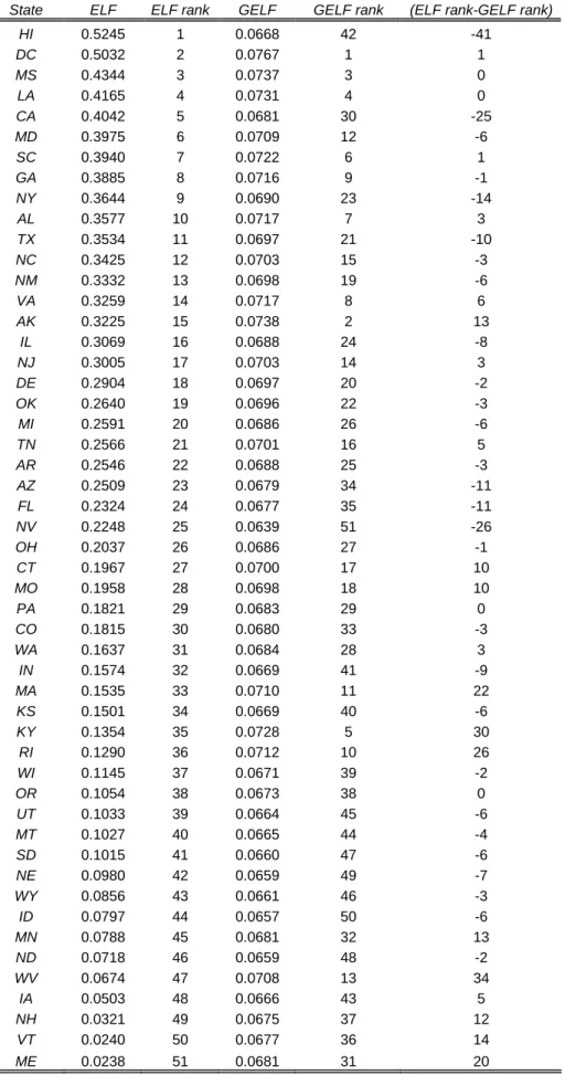
[Insert Table 1]
Table 1 provides the counterpart to the graphical analysis, as it reports the full set of states listed in decreasing order of ethno-linguistic fractionalization, the corresponding values of ELF , GELF and the difference in ranks between ELF and GELF for each state. We prefer to rely on a comparison of ranks because the absolute values of the two indices are not comparable. In particular, in the last column of table 1 we report the difference ELF rank − GELF rank, so that negative values indicate that a given state is less fractionalized according to GELF than according to ELF, while positive values indicate the opposite. The magnitude of the difference gives a rough approximation of how big a difference it makes for a particular state to use one index over the other, in terms of relative rankings.
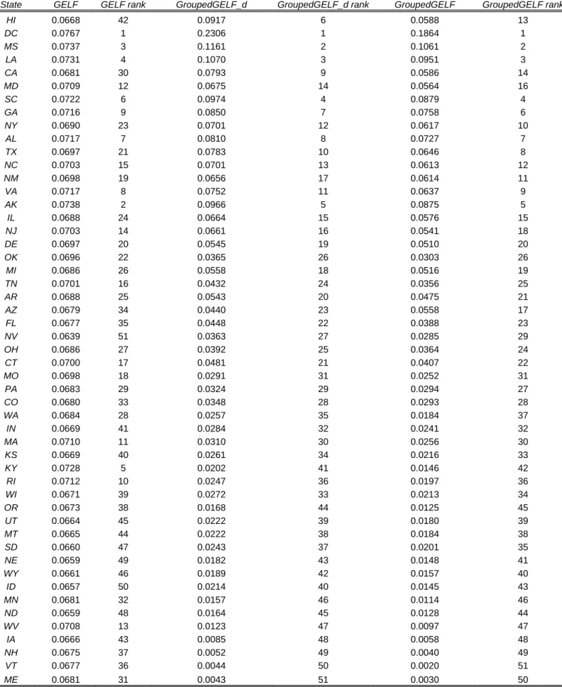
We next turn to an investigation of what happens when race is isolated to define relevant subgroups and distance is computed on the remaining components. In particular, we implement formula (2) with the slight modification that individuals are exogenously grouped into five categories–in this case racial groups–and distances among groups are measured as the difference in a synthetic measure of income, education and employment.7 The results are displayed in table 2.
[Insert Table 2]
States in table 2 are listed in decreasing order of GELF, and two additional in-dices (with the corresponding ranks) are reported. The first index, which we denote
7As before, this synthetic index is the first principal component extracted from our income, education
and employment variables, where we use a polychoric correlation matrix to take into account the fact that employment is a categorical variable.
as GroupedGELF _d, employs the Kolmogorov distance among distributions of the syn-thetic index to compute similarity values that are the used in formula (2). The second index, denoted as GroupedGELF, is simpler in that only the average value of the syn-thetic index for each racial group is used when computing distances (differences). While the use of means or of the entire distribution yield very similar results, the comparison with GELF suggests that for some states the exogenous definition of racial categories does make a difference: these are the same states for which the difference between ELF and GELF in figure 1 was more pronounced. In this sense, and not surprisingly, the GroupedGELF index calculated according to (2) is more similar to ELF than the GELF index (1) calculated on the full similarity matrix.
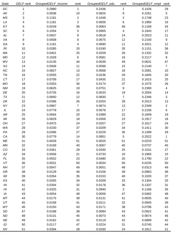
[Insert Table 3 and Figure 2]
Finally, in table 3 we try to disentangle the contribution of each individual dimension to overall diversity by implementing a version of (2) where distance among racial groups is measured solely in terms of differences in average income (GroupedGELF_income), differences in average years of education (GroupedGELF_edu), or difference in the share of people employed (GroupedGELF_empl ). For each index, we report the value and the rank, and states are still listed in decreasing order of the full similarity GELF. The results are quite informative and are more easily visualized through figure 2. Panel A of the figure plots the original values of ELF on the horizontal axis against GroupedGELF_income on the vertical one. The two measures are closely correlated with two extreme outliers: Hawaii is much less fractionalized when we use GroupedGELF_income than when we use ELF, while the opposite occurs for the District of Columbia. The intuition is similar to that provided when commenting on figure 1, i.e., in states like Hawaii or California average income levels are relatively more similar among races than they are in DC or in Connecticut, for example. A similar picture is offered in Panel B with respect to years of education. Interestingly, however, when we look at employment levels (Panel C) the relationship between the two indices becomes hump-shaped. The maximum value of diversity according to GroupedGELF_empl corresponds to intermediate levels of ethnic fractionalization; on the other hand, very low or very high levels of ELF translate into middle range values of diversity when both race and similarity in employment status are taken into account. A possible interpretation of this result is that sizeable differences in employment status (e.g., high unemployment levels for minorities) may be politically difficult to sustain in states where a relatively high fraction of the population is non-white. On the other hand, the same does not hold for income, as if income differences were more
easily acceptable compared to the universal right of access to employment.
While only suggestive and illustrative, the above analysis highlights some of the poten-tial benefits that may derive from the use of fractionalization indices that do not simply rely on population shares, but also try to incorporate information on other dimensions along which individuals may differ.
6
Concluding remarks
The main purpose of this paper is to provide a theoretical foundation and an empirical illustration of a new measure of ethnic diversity. Unlike the most commonly used ELF in-dex, our generalized version GELF makes use of a broader informational base. Instead of limiting the relevant variables to the population shares of predefined groups, we start out with a notion of similarity among individuals and calculate our index value accordingly. It is possible to derive a partition into groups endogenously, and the standard ELF index emerges as a special case when no partial similarity is allowed. The results of our empir-ical application suggest that accounting for the extent of similarity among individuals in observable dimensions other than race may indeed alter the picture of ‘ethnic diversity’ in the United States. In places like New England or Washington DC racial fractionalization is magnified when similarity in income, education or employment is taken into account; in places like California the opposite occurs.
Before concluding, we would like to stress an important methodological point. While in this paper we characterize GELF on the basis of similarities among individuals, our approach is silent on how these similarities should be defined. In particular, our approach is fully compatible with a setting in which the notion of continuous distance does not apply (i.e., individuals are either fully similar or fully dissimilar, in which case our prim-itives sij will take values 0 or 1), as well as with a setting in which it is meaningful to
think of similarity among individuals in a continuous way. In addition, our index allows to incorporate a multidimensional concept of similarity, as opposed to a single dimen-sion. We view this flexibility as an advantage of our approach, and one that makes our index applicable in many different settings. Our choice in the empirical illustration was guided by the attempt to compare our results with well known patterns in the economics literature on ethnic fractionalization in the US. We chose as dimensions of similarity eth-nicity, household income, education and employment status since we believe that these are important aspects of the US economy that could influence the behavior of individuals. However, the choice of variables to be employed in the measurement of similarity could
include very different aspects and should be guided by the specific application that one has in mind.
Finally, the application of our index is not limited to studies involving ethno-linguistic fractionalization. The generalized index that we propose may be applied to various areas in economics, including for example industrial organization. GELF is an index of diversity, and the difference between one and the index value can be interpreted as an index of concentration. Embedding information on similarity among firms in a concentration index may yield different results than the traditional Herfindahl index, which is purely based on market shares.
Appendix
In this appendix, we illustrate that our characterization result is unchanged if the set of similarity matrices Sn
consists of all n × n matrices S satisfying conditions (a) and (b) of section 2, but not necessarily (c). This is achieved by some straightforward modifications of the definition used in the proof of Theorem 1.
That any positive multiple of G satisfies the axioms on the larger domain as well is, again, straightforward to verify. Conversely, suppose D is a diversity measure defined on the larger domain satisfying normalization, anonymity, additivity and replication invari-ance. Let n ∈ N \ {1}, and define the set Xn⊆ Rn(n−1)/2 by
Xn = {x = (xij) i∈{1,...,n}
j∈{1,...,n}\{i} | ∃S ∈ S
n such that s
ij = xij for all i ∈ {1, . . . , n}
and for all j ∈ {1, . . . , n} \ {i}}. Define the function Fn:Xn→ R by letting, for all x ∈ Xn,
Fn(x) = D(S)− D(In) (12)
where S ∈ Sn is such that s
ij = xij for all i ∈ {1, . . . , n} and for all j ∈ {1, . . . , n} \ {i}.
Because D is bounded below by zero, it follows that Fn
is bounded below by −D(In).
Furthermore, the additivity of D implies that Fn satisfies Cauchy’s basic functional
equa-tion
Fn(x + y) = Fn(x) + Fn(y) (13)
for all x, y ∈ Xn
such that (x + y) ∈ Xn; see Aczél (1966, Section 2.1).
Fix i ∈ {1, . . . , n} and j ∈ {1, . . . , n} \ {i}, and define the function fn
ij: [0, 1]→ R by
for all xij ∈ [0, 1], where the vector (xij; 0n(n−1)−1)is such that the component
correspond-ing to ij is given by xij and all other entries (if any) are equal to zero. The function fijn
is bounded below because Fn is and, as an immediate consequence of (13), it satisfies the
Cauchy equation
fijn(xij + yij) = fijn(xij) + fijn(yij) (14)
for all xij, yij ∈ [0, 1] such that (xij + yij) ∈ [0, 1]. Because the domain of fijn is an
interval containing the origin and fn
ij is bounded below, the only solutions to (14) are
linear functions; see Aczél (1966, Section 2.1). Thus, there exists cn
ij ∈ R such that
Fn(xij; 0n(n−1)−1) = fijn(xij) = cnijxij (15)
for all xij ∈ [0, 1].
Let S ∈ Sn. By additivity, the definition of Fn and (15),
Fn³(sij) i∈{1,...,n} j∈{1,...,n}\{i} ´ = n X i=1 n X j=1 j6=i Fn(sij; 0n(n−1)−1) = n X i=1 n X j=1 j6=i fijn(sij) = n X i=1 n X j=1 j6=i cnijsij
and, defining dn = D(In) and substituting into (12), we obtain
D(S) = n X i=1 n X j=1 j6=i cnijsij + dn. (16)
Now fix i, k ∈ {1, . . . , n}, j ∈ {1, . . . , n} \ {i} and ∈ {1, . . . , n} \ {k}, and let S ∈ Sn be such that sij = 1 and all other off-diagonal entries of S are equal to zero. Let the
bijection π ∈ Πn be such that π(i) = k, π(j) = , π(k) = i, π( ) = j and π(h) = h for all h∈ {1, . . . , n} \ {i, j, k, }. By (16), we obtain
D(S) = cnij + dn and D(Sπ) = cnk + d n,
and anonymity implies cn
ij = cnk . Therefore, there exists cn∈ R such that cnij = cn for all
i∈ {1, . . . , n} and for all j ∈ {1, . . . , n} \ {i}, and substituting into (16) yields D(S) = cn n−1 X i=1 n X j=i+1 sij + dn
for all n ∈ N \ {1} and for all S ∈ Sn. Normalization requires
and, therefore, dn=
−cnn(n
−1) for all n ∈ N\{1}. Using normalization again, we obtain D(In) =−cnn(n− 1) > 0
which implies cn < 0
for all n ∈ N \ {1}. Thus, D(S) = cn n X i=1 n X j=1 j6=i sij − cnn(n− 1) (17)
for all n ∈ N \ {1} and for all S ∈ Sn.
Let n be an even integer greater than or equal to four. By replication invariance and (17), D(R2n/2) = cnn ³n 2 − 1 ´ − cnn(n− 1) = −c2 = D(I2). Solving, we obtain cn= 2c 2 n2. (18)
Now let n be an odd integer greater than or equal to three. Thus, q = 2n is even, and the above argument implies
cq= 2c
2
q2 =
c2
2n2. (19)
Furthermore, replication invariance requires
D(Rn2) = D(Rq/22 ) = cqq− cqq(q− 1) = −cnn(n− 1) = D(In).
Solving for cn and using the equality q = 2n, it follows that cn = 4cq and, combined with
(19), we obtain (18) for all odd n ∈ N \ {1} as well.
Substituting into (17), simplifying and defining α = −2c2 > 0, it follows that, for all n∈ N \ {1} and for all S ∈ Sn,
D(S) = 2c 2 n2 n X i=1 n X j=1 j6=i sij− cnn(n− 1) = 2c 2 n2 n X i=1 n X j=1 sij− 2 c2 n2n− 2 c2 n2n(n− 1) = −2c2 " 1− 1 n2 n X i=1 n X j=1 sij # = αG(S).
References
[1] Aczél, János (1966), Lectures on Functional Equations and Their Applications, Aca-demic Press, New York.
[2] Alesina, Alberto, Reza Baqir and William Easterly (1999), “Public Goods and Ethnic Divisions”, Quarterly Journal of Economics, 114, 1243—1284.
[3] Alesina, Alberto, Reza Baqir and Caroline Hoxby (2004), “Political Jurisdictions in Heterogeneous Communities”, Journal of Political Economy, 112, 348—396.
[4] Alesina, Alberto, Arnaud Devleeschauwer, William Easterly, Sergio Kurlat and Ro-main Wacziarg (2003), “Fractionalization”, Journal of Economic Growth, 8, 155—194. [5] Alesina, Alberto and Eliana La Ferrara (2000), “Participation in Heterogeneous
Com-munities”, Quarterly Journal of Economics, 115, 847—904.
[6] Alesina, Alberto and Eliana La Ferrara (2005), “Ethnic Diversity and Economic Performance”, Journal of Economic Literature, forthcoming.
[7] Bisin, Alberto and Thierry Verdier (2000), “Beyond the Melting Pot: Cultural Trans-mission, Marriage, and the Evolution of Ethnic and Religious Traits”, Quarterly Journal of Economics, 115(3), 955—988, 2000.
[8] Bossert, Walter, Prasanta K. Pattanaik and Yongsheng Xu (2003), “Similarity of Options and the Measurement of Diversity”, Journal of Theoretical Politics, 15, 405— 421.
[9] Caselli, Francesco and Wilbur J. Coleman (2002), “On the Theory of Ethnic Con-flict”, unpublished manuscript, Harvard University.
[10] Desmet, Klaus, Ignacio Ortuño-Ortín and Shlomo Weber (2005), “Peripheral Diver-sity and Redistribution”, CEPR, Discussion Paper No.5112.
[11] Easterly, William and Ross Levine (1997), “Africa’s Growth Tragedy: Policies and Ethnic Divisions”, Quarterly Journal of Economics, 111, 1203—1250.
[12] Esteban, Joan-Maria and Debraj Ray (1994), “On the Measurement of Polarization”, Econometrica, 62, 819—851.
[13] Fearon, James D. (2003), “Ethnic and Cultural Diversity by Country”, Journal of Economic Growth, 8, 195—222.
[14] Fernandez, Raquel, Alessandra Fogli and Claudia Olivetti (2004), “Mothers and Sons: Preference Transmission and Female Labor Force Dynamics?”, Quarterly Journal of Economics, 119(4), 1249—1299.
[15] Gini, Corrado (1912), “Variabilità e Mutabilità”, Studi Economico-Giuridici della Facoltà di Giurisprudenza dell’Università di Cagliari, a.III, parte II.
[16] Giuliano, Paola (2007), “Living Arrangements in Western Europe: Does Cultural Origin Matter?”, Journal of the European Economic Association, 5(5), 927—952. [17] Giuliano, Paola, Antonio Spilimbergo and Giovanni Tonon (2006), “Genetic, Cultural
and Geographical Distances,” IZA Discussion Papers 2229.
[18] Greenberg, Joseph H. (1956) “The Measurement of Linguistic Diversity”, Language, 32, 109—115.
[19] Guiso, Luigi, Paola Sapienza and Luigi Zingales (2004), “Cultural Biases in Economic Exchange,” NBER Working Paper No. 11005.
[20] Laitin, David (2000), “What is a Language Community?”, American Journal of Po-litical Science, 44, 142—154.
[21] Mauro, Paolo (1995), “Corruption and Growth”, Quarterly Journal of Economics, 110, 681—712.
[22] Montalvo, Jose G. and Marta Reynal-Querol (2005), “Ethnic Polarization, Potential Conflict, and Civil Wars”, American Economic Review, 95, 796—816.
[23] Montalvo, Jose G. and Marta Reynal-Querol (2007), “Discrete Polarization with an Application to the Determinants of Genocides”, mimeo, Universitat Pompeu Fabra. [24] Moody, James (2001), “Race, School Integration, and Friendship Segregation in
America”, American Journal of Sociology, 107, 679—716.
[25] Nehring, Klaus and Clemens Puppe (2002), “A Theory of Diversity”, Econometrica, 70, 1155—1198.
[26] Pattanaik, Prasanta K. and Yongsheng Xu (2000), “On Diversity and Freedom of Choice”, Mathematical Social Sciences, 40, 123—130.
[27] Rao, Radhakrishna C. (1982), “Diversity: Its Measurement, Decomposition, Appor-tionment and Analysis”, Sankhy¯a, 44, A, 1—22.
[28] Rao, Radhakrishna C. (1984), “Convexity Properties of Entropy Functions and Analysis of Diversity”, in Inequalities in Statistics and Probability, Y.L. Tong Ed., IMS Lecture Notes, 5, 68—77.
[29] Rao, Radhakrishna C. and Tapan K. Nayak (1985), “Cross Entropy, Dissimilarity Measures, and Characterizations of Quadratic Entropy”, IEEE Transactions on In-formation Theory, IT-31, 5, 589—593.
[30] Reynal-Querol, Marta (2002), “Ethnicity, Political Systems and Civil War”, Journal of Conflict Resolution, 46(1), 29—54.
[31] Simpson, Edward H.(1949), “Measurement of Diversity”, Nature, 163, 688.
[32] Spolaore, Enrico and Romain Wacziarg (2006), “The Diffusion of Development”, NBER Working Paper No. 12153.
[33] Vigdor, Jacob L. (2002), “Interpreting Ethnic Fragmentation Effects”, Economics Letters, 75, 271—76.
[34] Weitzman, Martin (1992), “On Diversity”, Quarterly Journal of Economics, 107, 363—405.
Figure 1: GELF and ELF in the US. GE L F ELF .023752 .524481 .06393 .076675 HI DC MS LA CA MD SC GA NY AL TX NC NM VA AK IL NJ DE OK MI TN AR AZ FL NV OH CT MO PA CO WA IN MA KS KY RI WI OR UT MT SD NE WY ID MN ND WV IA NH VT ME
Figure 2: GroupedGELF (income, education, employment) and ELF in the US. Panel A G E LF g rou p e d, i n c o m e ELF .023752 .524481 .002819 .288038 HI DC MS LA CA MD SC GA NY AL TX NC NM VA AK IL NJ DE OK MI TN AR AZ FL NV OH CT MO PA CO WA IN MA KS KY RI WI OR UT MT SD NE WY ID MN ND WV IA NH VT ME