OATAO is an open access repository that collects the work of Toulouse
researchers and makes it freely available over the web where possible
Any correspondence concerning this service should be sent
to the repository administrator:
[email protected]
This is an author’s version published in: http://oatao.univ-toulouse.fr/20017
To cite this version:
Ben Abdallah, Mohamed and Ayadi, Mounir and Rotella,
Frédéric
and Benrejeb, Mohamed LTV controller flatness-based
design for MIMO systems. (2014) International Journal of Dynamics
and Control, 2. 335-345. ISSN 2195-268X
LTV controller flatness-based design for MIMO systems
Mohamed Ben Abdallah · Mounir Ayadi · Frédéric Rotella · Mohamed Benrejeb
Abstract In this paper, a flatness-based control strategy for multi-input multi-output linear time-varying systems is proposed in order to track desired trajectories. The control design, based on the use of an exact observer, leads to a poly-nomial two-degree-of-freedom controller without resolving Bézout’s equation in a time-varying framework. The pro-posed approach is illustrated with the control of a nonlinear model of the satellite SPOT-5.
Keywords Linear time-varying systems · Multi-input multi-output systems · Trajectory linearization · Flatness · Path tracking · Exact observer · Polynomial controller
1 Introduction
For finite-dimensional and time-invariant linear systems, a well-known control design technique named polynomial two-degree-of-freedom (2DOF) controllers [1–3], was intro-duced fifty years ago by Horowitz [4]. This powerful method is based on pole placement and presents one drawback: it needs to know where to place all the poles of the closed-loop system at the outset. In dealing with polynomial matrices in M. Ben Abdallah (
B
) · M. Ayadi · M. BenrejebLR-11-ES18 Laboratoire Automatique, École Nationale d’Ingénieurs de Tunis, Université de Tunis El Manar, 1002 Tunis, Tunisia e-mail: [email protected] M. Ayadi e-mail: [email protected] M. Benrejeb e-mail: [email protected] F. Rotella
EA 1905 Laboratoire Genie de Production,
École Nationale d’Ingénieurs de Tarbes, 65016 Tarbes, France e-mail: [email protected]
the case of multi-input multi-output (MIMO) systems, a par-ticular problem which is important for both, mathematical [5,6] and system theory [7,8] points of view, is the computa-tion of the solucomputa-tion of the generalized polynomial Bézout’s equation. There are many works to solve the diophantine equation [9,10]. Generally, all methods can be classified into three main categories: the state-space related approaches [11,12], the Taylor series treatment [10,13], and methods involving coefficient matching [9,14].
The 2DOF design controller problem is not easy to tran-scribe in the case of linear time-varying (LTV) systems due to the fact that the coefficients do not commute with the time derivative operator. Besides, the structure of the set of the poles of the closed-loop system is more complex.
In this case, the pole placement problem was solved
recently by Marinescu [15] who proposes some technical
methods for the factorization of linear time-varying transfer matrices. These key points lead to solve Bézout’s equation written in time-varying framework.
In the case of single-input single-output (SISO) linear time-invariant (LTI) systems, the problem of pole placement which consists in imposing closed loop system dynamics can be related to track desired trajectories using flatness property to design a polynomial controller [16]. A 2DOF controller is then designed with very natural choices with high level performances. In this design, we are led to a solution for Bézout’s equation without its resolution.
In order to overcome these two points, namely the choice of desired poles at the outset and the determination of a solu-tion for Bézout’s equasolu-tion, we propose in this paper to extend the flatness-based control strategy developed in [16] to the case of MIMO LTV systems. It will be seen that applying the guideline induced by a flatness based control to a MIMO LTV system leads to express it in a natural 2DOF controller form.
The paper is organized as follows: in Sect.2, some back-ground notions about MIMO LTV systems and flatness are
presented. In Sect.3, we propose to design a polynomial
controller based on flatness using an exact observer of a state vector which is constituted by the flat output and its deriva-tives. This approach is illustrated, in Sect.4, with the control of a nonlinear model of the SPOT satellite.
2 Background notions
2.1 MIMO linear time-varying systems
Following [15], in the algebraic framework initiated by [17] and popularized in systems theory by [18] and related refer-ences, a linear system is a finitely presented module M over the ring R = K [s] of differential operators in s = d/dt with coefficients in an ordinary differential field K (i.e., a com-mutative field equipped with a unique derivative). If K does not exclusively contain constants (i.e., elements of deriva-tive zero), M is an LTV system. In this paper, the following notations will be used: u(n)(t ) = dndtu(t )n = snu(t ).
When dealing with LTV systems, polynomials as function of s is skew, i.e., belong to the noncommutative ring R =
K [s] equipped with the commutation rule: sa = as + ˙a
(a is a time-varying function), which is the Leibniz rule of derivation of a product. Noting the integration operator by s−1where: s−1h (t ) = t ! −∞ h (τ )dτ (1)
where h(τ ) = 0 for (τ ≤ ¯τ ). This last hypothesis ensures commutativity between s and s−1.
For finite-dimensional, several input-output descriptions have been introduced for MIMO LTV systems. Here, a time-varying linear system is described by the following state space model of dimension n:
˙x(t) = A(t)x(t) + B(t)u(t) t ∈ T =" t1 t2#
y(t ) = C(t )x(t ) (2)
where x(t ) is an n-dimensional state vector, u(t ) is an m-dimensional input vector, y(t ) is an m-m-dimensional output vector, and the matrices A(t ), B(t ) and C(t ) are time-variable matrices of proper order. Consider the set of matrices Ki(t ) for i = 0, 1, . . . such that:
K0(t ) = B(t )
Ki(t ) = − A(t )Ki −1(t ) + ˙Ki −1(t ) if i ≥ 1 If there is an integer µ such that the matrix:
K( A(t ),B(t ))(t ) =$K0(t ) · · · Kµ−1(t )% (3)
is of rank n for every t ∈ T , then the system is uniformly con-trollable [19] and K( A(t ),B(t ))(t )is the controllability matrix. Consider the set of matrices Li(t ), for i = 0, 1, . . . such that: L0(t ) = C (t )
Li(t ) = Li −1(t ) A (t ) + ˙Li −1(t ) if i ≥ 1 If there is an integer ν such that the matrix:
L( A(t ),C(t ))(t ) = L0(t ) L1(t ) .. . Lν−1(t ) (4)
is of rank n for every t ∈ T , then the system is uniformly observable. In this condition, L( A(t ),C(t ))(t )is the observ-ability matrix of the pair ( A(t ), C(t )). In the case of LTI systems, the indexes µ and ν are equal to n. The result of
Silverman-Meadows [19] has shown that, if the system is
uniformly controllable then there exists a nonsingular trans-formation on T , such that:
Z (t ) = PC(t )x(t ) (5)
which can be constructed by the Seal-Stuberud algorithm [20], implies that: ˙ Z (t ) = AC(t )Z (t ) + BC(t )u(t ) y(t ) = CC(t )Z (t ) (6) where: CC(t ) = C (t ) PC−1(t ) , BC(t ) = PC(t )B(t ) (7) AC(t ) = PC(t ) A(t )PC−1(t ) + ˙PC(t )PC−1(t ) =" ACi j(t )#i, j =1...m (8) AC,i i(t ) = 0 1 0 · · · 0 .. . . .. . .. . .. ... .. . . .. . .. 0 0 · · · 0 1 × × × × × (9)
are µi× µimatrices such that: n , i =1 µi = n AC,i j(t ) = 0 · · · 0 .. . ... .. . ... 0 · · · 0 × × · · · × × (10)
are (µi× µj)matrices, the symbol × is a time-varying
indices determined by the the Seal-Stuberud algorithm [20]. The interested reader may find more details about this algo-rithm in the quoted literature and the references therein.
Defining a new input vector uC(t )by:
uC(t ) = HC(t )u(t ) (11)
where HC(t )is an (m × m) upper triangular matrix with ones
along the diagonal and hence invertible. It’s constructed by the-i j =1µjth rows of BC(t ): HC(t ) = 1 × · · · × 0 . .. ... .. . . .. . .. × 0 · · · 0 1 (12) Equation (6) becomes: ˙ Z (t ) = ACZ (t ) + ¯BCuC(t ) y(t ) = CCZ (t ) (13) such that: ¯ BC = BC(t )HC(t )−1 = bc1 0 · · · 0 0 bc2· · · 0 .. . ... ... 0 0 bcm (14) where: bci =. 0 · · · 0 1 / T (15) is an µivector.
Remark 1 Another problem is that even though the
time-varying linear system is controllable and observable, its con-trollability indices and/or observability indices may not be fixed. Such system is called non-lexicographically-fixed sys-tem. For this problem, the algorithm of Seal and Stuberud can’t be implemented in an efficient way because the set of vectors which are linearly independent for every t on T change. In this work, we only deal lexicographically-fixed system [21] where the controllability indices are fixed. In the next section, the flatness property is presented and we will see that the state vector in the previous canonical form is used to determine the flat output and its derivatives.
2.2 Short survey on flatness
Flatness property which was introduced by [22], for continu-ous-time nonlinear systems, leads to interesting results for control design. The existence of a set of variables called flat outputs permits to define all other system variables. The dynamic of such process can be then deduced without solving the differential equations. Therefore, it is possible to express
the state, as well as the input and the output of the system, as differential functions of flat outputs [22,23]. Let us consider the nonlinear system described by the following differential equation:
˙x(t) = f (x(t), u(t)) (16)
where x(t ) ∈ ℜnis the state vector and u(t ) ∈ ℜmis the input vector. Roughly speaking, this system is called differentially flat if there exists a set of variables z(t ) ∈ ℜmof the form:
z(t ) = h(x(t ), u(t ), ˙u(t ), ..., u(r )(t )) (17)
such that the state and the input of the system are given by:
x(t ) = A(z(t ), ˙z(t ), ..., z(α)(t )) (18)
u(t ) = B(z(t ), ˙z(t ), ..., z(α+1)(t )) (19)
where α is an integer. The set of variables z(t ) is called the flat output of the system or the endogenous variables. It makes possible to parameterize any variable of the system [23]. The components of z(t ) must be differentially independent. The real output of the process is written as follows:
y (t ) = g (x (t ) , u (t )) (20)
and from Eqs. (18) and (19), this output is written in function of the flat output as:
y(t ) = C(z(t ), ˙z(t ), ..., z(σ )(t )) (21)
where σ is an integer. In the linear case, the explicit expres-sions of the output y(t ) and the input u(t ) allow to relate the flat output to the partial state which was defined by [7]. The trajectories of the system are deduced from the definition of the flat output trajectory without integrating any differen-tial equations. All these points, which have been formalized through the Lie-Bäcklund equivalence of systems in [24,25], lead to propose a nonlinear feedback which ensures a stabi-lized tracking of a desired motion for the flat output. This methodology has been applied on many industrial processes as it was shown previously, for instance, on magnetics bear-ings [26], chemical reactors [27], cranes or flight control [28] or turning process [29], among many other examples.
A necessary and sufficient condition for the flatness of a linear system is its controllability involving that the con-cepts flatness and controllability coincide [30]. In this case, the Brunovsky output from the controllable canonical form are considered as flat outputs. The Lie-Bäcklund equivalence [24] shown that: di m z(t ) = di m u(t ).
In the case of MIMO linear systems, let us consider the canon-ical form in Eq. (13), the state vector can be expressed in the following form:
Z (t ) = z1(t ) .. . z(µ1−1) 1 (t ) z2(t ) .. . zm(t ) .. . z(µm−1) m (t ) (22)
then the flat output or the Brunovsky output is given by:
z(t ) = z1(t ) z2(t ) .. . zm(t ) (23)
Remark 2 The necessary and sufficient condition for the
flat-ness of a linear system is proved in the LTI case in [30]. In the LTV case, uniform controllability implies, according to the results of Malrait et al. in [31], that the system is equivalent to a linear time invariant system in Brunovsky canonical form (i.e. a chain of n integrators) after a static change of coordi-nates and a state-dependent re-definition of the control input. The system is thus differentially flat [32]. The flat output, or Brunovsky output, is directly obtained as a time-varying lin-ear combination of the original states.
After introducing the flatness property and the determina-tion of a flat output from the controllable form, the flatness-based control will be presented in the next section.
3 Flatness-based control
By denoting by uC,i(t ) the i-th component of uC(t ) and
αi, j,k(t ) the k-th coefficient of the last row of the matrix
AC,i j(t ) in Eq. (9) and Eq. (10), the following relation is
satisfied: uc,i(t ) = z(µi i)(t ) + m , j =1 µi−1 , k=0 αi, j,k(t )z(k)j (t ) (24)
For a given planned trajectory of the flat output, zd(t ), the
control law based on flatness is as follows: uc,i(t ) = z(µd,ii)(t ) + µi , k=0 κi,k $ z(k)d,i(t ) − z(k)i (t )% + m , j =1 µj−1 , k=0 αi, j,k(t )z(k)j (t ) (25)
where the κi,k are chosen such that:
κi(s) = sµi +-k=µi1κi,ksµi−kis a Hurwitz polynomial. By
introducing the polynomial matrix:
K (s) = di ag (κi(s)) (26)
where s is the derivation operator, the previous control law can be written as:
u(t ) = (HC)−1(t ) (K (s)zd(t ) − 3(t )Z (t )) (27) where: 3(t ) ="3i, j(t )#i, j =1···m =
"κi,0− αi,i,0(t ) · · · κi,µi−1− αi,i,µi−1(t )
# if i = j "−αi, j,0(t ) · · · −αi, j,µi−1(t ) # if i 6= j (28) When this control is applied, the tracking error is verifying:
lim
t →∞(zd(t ) − z (t )) =0 (29)
and the closed-loop dynamics are given by the roots of κi(s).
To implement the control (27), we need to estimate the vector
Z (t )with an observer. A full-order observer can be used, but
in this solution, the difficulty appears in the choice of the observers poles in the LTV framework. To overcome this point, an enlightening idea suggested in [33] and applied in [34] and [16] can be used. The realization of this controller, using the exact observer, will be the subject of the next part. 3.1 Exact observers
By successive derivations of the output plant y(t ) in the equa-tion (13) until the order (ν − 1), we get:
y (t ) = CC(t ) Z (t ) = O0(t ) Z (t ) ˙y (t) =.˙ CC(t ) + CC(t ) AC(t )/ Z (t) + CC(t ) ¯BCuC(t ) = O1(t ) Z (t ) + M1(t ) uC(t ) y(2)(t ) =. ˙ O1(t ) + AC(t ) O1(t )/ Z (t) + . O1(t ) ¯BC(t ) + ˙M1(t )/ uC(t ) + M1(t ) ˙uC(t ) = O2(t ) Z (t ) + M2(t ) uC(t ) + M1(t ) ˙uC(t ) .. . y(ν−1)(t ) = Oν−1(t ) Z (t ) + Mν−1(t ) uC(t ) + Mν−1,2(t ) ˙uC(t ) + Mν−1,3(t ) u(2)C (t ) + · · · + M1(t ) u(ν−2)C (t ) (30)
where Mi(t )are (m × m)-dimensional matrices given by:
– M1(t ) = CC(t ) ¯BC, – for i = 2 to ν − 1, Mi(t ) = ˙Mi −1(t ) + Oi(t ) ¯BC, – Mν−1,2(t ) = Mν−2(t ) +-ν−3i =1 M (ν−2−i ) i (t ), – Mν−1,3(t ) = Mν−3(t ) +-ν−4i =1(ν − i −2) M (ν−3−i ) i (t ), etc.
Equation (30) can be written as follows:
where YT(t ) =. yT(t ) ˙yT(t ) · · · y(ν−1)T(t )/ (32) UT(t ) =$uCT(t ) ˙uTC(t ) · · · u(ν−2)TC (t ) % (33) O (t ) = O0(t ) O1(t ) .. . Oν−1(t ) (34)
O (t )is the observability matrix of the pair
( AC(t ) , CC(t ))and M (t ) is the transmission matrix given
by: M(t ) = M0 M0 · · · M0 M0 M1(t ) M0 M0 . . . . .. . .. ... Mν−2(t ) M1(t ) M0 Mν−1(t ) Mν−1,2(t ) Mν−1,3(t ) · · · M1(t ) (35)
such that M0is an (m × m)-dimensional zero matrix. In the next development, we assume the uniform observ-ability of the system leading to:
r ank (O (t )) = n (36)
such that O (t ) is an (mν × n)-dimensional matrix. It appears that:
r ank (O (t )) = r ank." O (t) Y (t) − M (t) U (t) #/
= n
thus, following [35], the system of linear equations (31) is said compatible having a unique and an exact solution for
Z (t )given by:
Z (t ) =$OT(t ) O (t )%−1OT (t ) (Y (t ) − M (t ) U (t ))
(37) Besides, by integrating Eq. (13) of the canonical form, we get:
Z (t ) = s−1( AC(t ) Z (t )) + s−1.B¯CuC(t )/ (38)
By replacing, in the right side of Eq. (38), Z (t ), by the expres-sion from the left side, we obtain:
Z (t ) = s−1$AC(t ) s−1( AC(t ) Z (t ))
%
+ s−1AC(t ) s−1.B¯CuC(t )/ + s−1.B¯CuC(t )/(39)
Reiterating the last operation until the (ν − 1) order:
Z (t ) = s−1. AC(t )s−1( AC(t ) · · · s−1( AC(t )Z (t ))
+ s−1. AC(t )s−1( AC(t ) · · · s−1. AC(t ) ¯BCs−1uC(t )
//
+ · · · + s−1. AC(t ) ¯BCs−1uC(t )/
+ ¯BCs−1uC(t ) (40)
By replacing, in the second term of Eq. (40), Z (t ) by the expression from Eq. (37), implies that:
Z (t ) = s−1$AC(t )s−1( AC(t ) . . . s−1 3 AC(t ) $ OT(t ) O (t )% −1 OT(t ) (Y (t )−M (t ) U (t )) 44 + s−1$AC(t )s−1( AC(t ) · · · s−1 $ AC(t ) ¯BCs−1uC(t ) % + · · · + s−1$AC(t ) ¯BCs−1uC(t ) % + ¯BCs−1uC(t ) (41)
By using integration by parts, it leads to the following expres-sion of the state vector:
Z (t ) = s−1(Θ1(t ) y (t )) + s−2(Θ2(t ) y (t )) + · · ·
· · · + s−ν(Θν(t ) y (t )) + s−1(∆1(t ) uC(t ))
· · · + s−2(∆2(t ) uC(t )) + · · ·
· · · + s−(ν−1)(∆ν−1(t ) uC(t )) + ¯BCs−1uC(t )
(42) where Θi(t )and ∆i(t )are (n × m)-dimensional matrices.
3.2 2DOF controller form in the LTV case
By replacing (42) into (27), the control law becomes:
u(t ) =$HC(t ) %−1 (K (s)zd(t ) − 3(t ) 5 s−1(Θ1(t ) y (t )) + s−2(Θ2(t ) y (t )) + · · · + s−ν(Θν(t ) y (t )) + s−1(∆1(t ) uC(t )) + s−2(∆2(t ) uC(t )) + · · · + s−(ν−1)(∆ν−1(t ) uC(t ))+ ¯BCs−1uC(t ) 6% (43) By denoting: R.s−1, u (t )/ = u(t) + (HC(t ))−13(t ) ×.s−1(∆ 1(t ) uC(t ))+s−2(∆2(t ) uC(t )) + · · · + s−(ν−1)(∆ν−1(t ) uC(t )) + ¯BCs−1uC(t )/ (44) and S$s−1, y (t )%= (HC(t ))−13(t ) $ s−1(Θ1(t ) y (t )) + s−2(Θ2(t ) y (t )) + · · · + s−ν(Θν(t ) y(t )) / (45) the control law (43) can be written finally in the 2DOF con-troller form as follows:
R$s−1, u (t )%= (HC(t ))−1K (s)zd(t ) − S
$
s−1, y (t )% (46) The proposed control design can be seen as a 2DOF controller in the LTV framework without the resolution of Bézout’s equation. Now the design is focused on the choice of the
trajectory zd(t )to follow and the tracking dynamics given
by K (s).
4 Application: control of a nonlinear model of a satellite
4.1 Nonlinear model of a satellite
In this section, the proposed approach in the case of MIMO LTV systems is applied to the model of a satellite SPOT-5. SPOT (Système Pour l’Observation de la Terre) is a high-resolution, optical imaging Earth observation satellite system operating from space. Spot-5 satellites are the third genera-tion of SPOT satellites. Following [32,36,37], the nonlinear model of the satellite is given by:
¨r = r (t) ω2(t ) − k r2(t )+ u1(t ) m ˙ ω (t ) = −2˙r (t) ω (t) r (t ) + u2(t ) mr2(t ) (47) where:
– r (t) represents the distance from the center of the Earth. – θ (t) is the angular displacement with respect to an
arbi-trary but fixed direction in the orbiting plane. – m is the mass of the satellite (3,048 kg),
– k is a gravitational constant determining the Earth force of attraction on the satellite given by k = G MT such that
G = 6.672559 × 10⁻¹¹m3/s2 kg and MT = 5.9736 ×
1024kg is the mass of the Earth.
– ω (t) is the angular velocity, ω (t ) = ˙θ (t ).
(r (t ) , θ (t ))is the polar coordinates for the position of the satellite. The control inputs u1(t )and u2(t )represent the radial and tangential thrust forces exercised by the satellite respectively. By denoting:
x1(t ) = r (t ) = y1(t )
x2(t ) = ˙x1(t ) = ˙r (t ) (48)
x3(t ) = ω = y2(t )
the model of the system (47) can be written into the following form: ˙x1(t ) = x2(t ) ˙x2(t ) = x1(t ) x23(t ) − k x21(t )+ u1(t ) m (49) ˙x3(t ) = −2x2(t ) x3(t ) x1(t ) + u2(t ) mx12(t )
and their derivatives. Denoting: 7 z1(t ) = r (t )
z2(t ) = θ (t )
(50) then the system variables can be written as:
x1(t ) = z1(t ) x2(t ) = ˙z1(t ) x3(t ) = ˙z2(t ) (51) u1(t ) = m 8 ¨z1(t ) − z1(t ) ˙z22(t ) + k z21(t ) 9 u2(t ) = mz21(t ) 3 ¨z2(t ) + 2˙z1(t ) ˙z2(t ) z1(t ) 4
4.2 Linearization around a given trajectory
Consider the desired trajectories for the two flat outputs, suf-ficiently differentiable, which take the system from an initial state to an equilibrium final state defined by:
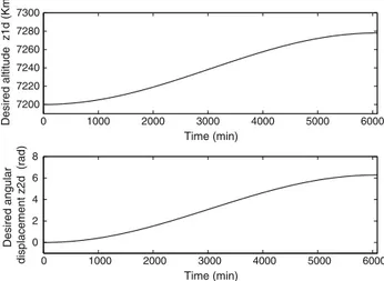
z1d(t ) = rd(t ) =.− cos .6084π t / + 1/ × 39 + 7200
z2d(t ) = θd(t ) =.− cos .6084π t / + 1/ × π
(52) Figure1 shows the desired trajectories of the flat outputs. From Eq. (51), the trajectories
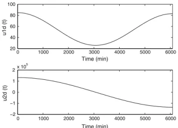
Td(t ) = (x1d(t ) , x2d(t ) , x3d(t ) , u1d(t ) , u2d(t )) can be then deduced. Figure2shows the desired trajectories for the inputs of the nonlinear system.
Let us define in the following the set of variables: δxi(t ) = xi d(t ) − xi(t ) for i = 1, 2, 3
δui(t ) = u1d(t ) − u1(t ) for i = 1, 2
The linearized model of (51) around the desired trajectories Td(t )is given by 0 1000 2000 3000 4000 5000 6000 7200 7220 7240 7260 7280 7300 Time (min) Desired altitude z1d (Km) 0 1000 2000 3000 4000 5000 6000 0 2 4 6 8 Time (min) Desired angular displacement z2d (rad)
Fig. 1 Desired trajectories of the two flat outputs z1d(t )and z2d(t )
A set of flat outputs for (47) can be easily found as
(r (t) , θ (t)) then the considered model is flat. Indeed, all the system variables are expressed in terms of these variables
0 1000 2000 3000 4000 5000 6000 20 40 60 80 100 Time (min) u1d (t) 0 1000 2000 3000 4000 5000 6000 −2 −1 0 1 2x 10 5 Time (min) u2d (t)
Fig. 2 Desired trajectories of the radial and tangential thrust forces,
u1d(t )and u2d(t ) δ ˙x1(t ) = δx2(t ) δ ˙x2(t ) = 8 x3d2 + 2 k x1d3 9 δx1(t ) + (2x1dx3d) δx3(t ) +δu1(t ) m δ ˙x3(t ) = 8 −2u2d mx1d3 + 2x2dx3d x1d2 9 δx1(t ) − 2x3d x1d δx2(t ) −3 2x2d x1d 4 δx3(t ) + 1 mx1d2 δu2(t ) (53) By denoting: δx (t ) = (δx1(t )δx2(t )δx3(t ))T (54)
the state space representation of the system can be written as:
δ ˙x (t ) = A (t ) δx (t ) + B (t ) u (t )
δy (t ) = C (t ) δx (t ) (55)
where:
δy (t ) = (δ y1(t )δ y2(t ))T δu (t ) = (δu1(t )δu2(t ))T
(56) A(t ) = 0 1 0 (x3d2 + 2 k x1d3 ) 0 (2x1dx3d) 3 −2u2d mx3 1d +2x2dx3d x2 1d 4 −2x3d x1d − $ 2x2d x1d % (57) B(t ) = 0 0 1 m 0 0 1 mx2 1d (58) C(t ) =3 1 0 0 0 0 1 4 (59) Clearly that r ank (B (t )) = 2.
Now, partition B (t) into column vectors:
B (t ) =[b1(t )b2(t )] (60)
To check the uniform controllability, we construct: K{2}(t ) = (K0(t ) K1(t )) = 0 0 −m1 0 1 m 0 0 − 2x3d mx1d 0 1 mx2 1d 2x3d mx1d 2(x2d− ˙x1d) mx3 1d (61)
The controllability matrix K{2}(t ) has rank 3 ∀ t, then
the system (55) is uniformly controllable and the
time-varying linearized system (53) is flat. According the pro-cedure referred in [20], the two indices of controllability are calculated: µ1= 2 and µ2= 1.
We construct the matrix V (t):
V (t ) = 0 −m1 0 1 m 0 0 0 2x3d mx1d 1 mx21d (62)
Clearly, V (t) is invertible ∀ t. After calculating V−1(t ), the second and third rows of this matrix are extracted to con-struct the matrix Pc(t ). The transformation Pc(t )reduces
the system (55) to the canonical form:
δ ˙Z (t ) = AC(t ) δ Z (t ) + ¯BC(t ) δuC(t ) δy (t ) = CC(t ) δ Z (t ) (63) where: AC(t ) = PC(t ) A(t )PC−1(t ) + ˙PC(t )PC−1(t ) AC(t ) = 0 1 0 α11,0(t ) α11,1(t ) α12,0(t ) α21,0(t ) α21,1(t ) α22,0(t ) ¯ BC(t ) = 0 0 1 0 0 1 , HC=3 1 0 0 1 4 CC(t ) = C (t ) PC−1(t )
4.3 Trajectory tracking by LTV flatness-based control Let’s denote δ Z (t ) the vector containing the flat outputs of the linearized system:
δ Z (t ) = (δz1(t )δ ˙z1(t )δz2(t ))T (64)
The previous control law (25) can be written as: uC1(t ) = ¨z1d(t ) + κ1,0z1d(t ) + κ1,1˙z1d(t )
−.κ1,0z1(t ) + κ1,1˙z1(t )/ + α1,1,0(t ) z1(t )
becomes: uC1(t ) − uC1,d(t ) = κ1,0δz1(t ) + κ1,1δ ˙z1(t ) − α1,1,0(t ) δz1(t ) − α1,1,1(t ) δ ˙z1(t ) − α1,2,0(t ) δz2(t ) (66) to obtain: δuC1(t ) =.α1,1,0(t ) − κ1,0/ δz1(t ) +.α1,1,1(t ) − κ1,1/ δ ˙z1(t ) + α1,2,0(t ) δz2(t ) (67) the same: δuC2(t ) =.α2,2,0(t ) − κ2,0/ δz2(t ) + α2,1,0(t ) δz1(t ) + α2,1,1(t ) δ ˙z1(t ) (68) implies that: δuC(t ) = 3 (t ) δ Z (t ) (69) where:
δuC(t ) =[δuC1(t )δuC2(t )]T (70)
3 (t ) = .α1,1,0(t ) − κ1,0/ α2,1,0(t ) .α1,1,1(t ) − κ1,1/ α2,1,1(t ) α1,2,0(t ) .α2,2,0(t ) − κ2,0/ T (71) We construct the observability matrix of the pair ( A(t ), C(t )): L{2}(t ) = 1 0 0 0 0 1 0 1 0 3 −2u2d mx1d3 + 2x2dx3d x1d2 4 −2x3d x1d − $ 2x2d x1d % (72) has r ank 3 ∀ t, the system is then uniformly observable. (31) can be written as:
δY (t ) = O(t )δ Z (t ) + M(t )δuC(t ) (73)
where: δY (t ) =3 δy (t) δ ˙y (t ) 4 , O(t ) = 3 CC(t ) ˙ CC(t ) + CC(t ) AC(t ) 4 and: M(t ) = 3 M0 CC(t ) ¯BC 4
O(t )is the observability matrix of the set ( AC(t ) , CC(t )).
By denoting as: $
OT(t ) O (t )%−1· OT(t ) = F (t ) (74)
(75)
Equation (63) can be written as:
δ Z (t ) = s−1. AC(t ) δ Z (t ) + ¯BCδuC(t )/ (76)
By replacing the expression of δ Z (t), from Eq. (75), in the right side of Eq. (76), we get:
δ Z (t ) = s−1( AC(t ) F (t )δY (t )) − s−1[ AC(t ) F (t )M(t )δuC(t )] + s−1.¯ BδuC(t )/ (77) with: AC(t ) F (t ) = τ1(t ) τ2(t ) τ3(t ) τ4(t ) τ5(t ) τ6(t ) (78) A (t ) F (t ) M (t ) = β1(t ) β2(t ) β3(t ) (79)
where τi(t ) and βi(t )are (1 × 2) time-varying matrices. By
using integration by parts such that δ ˙y(0) = 0, Eq. (77) leads to the following expression:
δ Z (t ) = τ2(t ) τ4(t ) τ6(t ) δy (t ) + s−1 τ1(t ) − ˙τ2(t ) τ3(t ) − ˙τ4(t ) τ5(t ) − ˙τ6(t ) δy(t ) + s−1 −β1(t ) −β2(t ) −β3(t ) δuC(t ) + s−1.¯ BCδuC(t )/ (80)
By replacing the expression of δ Z (t) into the control law (69): δu (t ) = HC−13 (t ) τ2(t ) τ4(t ) τ6(t ) δy (t ) + s−1 τ1(t ) − ˙τ2(t ) τ3(t ) − ˙τ4(t ) τ5(t ) − ˙τ6(t ) δy(t ) + s−1 −β1(t ) −β2(t ) −β3(t ) δuC(t ) + s−1.¯ BCδuC(t )/ % (81) we deduce that:
δu (t ) = S$s−1, δy (t )%+ R$s−1, δuC(t )
%
(82) we get:
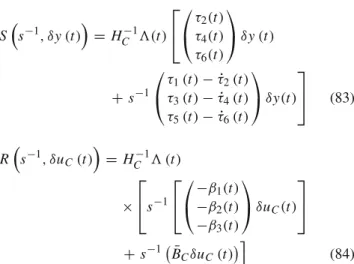
where: S$s−1, δy (t )%= HC−13(t ) τ2(t ) τ4(t ) τ6(t ) δy (t ) + s−1 τ1(t ) − ˙τ2(t ) τ3(t ) − ˙τ4(t ) τ5(t ) − ˙τ6(t ) δy(t ) (83) R$s−1, δuC(t ) % = HC−13 (t ) × s−1 −β1(t ) −β2(t ) −β3(t ) δuC(t ) + s−1.¯ BCδuC(t ) /6 (84)
Figure 3 illustrates the structure of the proposed method
based on the flatness property with the use of an exact observer.
The tracking model is set with the two polynomials κ1(s) = s2+ κ1,1s + κ1,0and κ2(s) = s + κ2,0.
For the numerical simulations, the tracking model is set
with a time response of 100 min for κ1(s)and 200 min
for κ2(s). The errors resulting from the inaccurate measure-ments perturbations used in the simulations are δy1(0) = 10 km and δy2(0) = −0.2 rad/s (the initial conditions due to the inaccurate measurements). The results obtained in Figs.
4,5,6and7, show that the trajectories of the nonlinear system follow the desired trajectories with good performance.
The control law obtained by application of the flatness-based controller, allows to obtain high performance in terms of path tracking with errors which tend asymptotically to zero (see Fig.7). These results point out the effectiveness of the use of the flatness-based approach for the LTV systems in a path tracking context.
The robustness of the control scheme is investigated when there is a change in the mass of the satellite, m, from (3,048 kg) to (3,000 kg) and in the gravitational constant, k, from 1443493.11439264 m3/s2to 1443220.28 m3/s2at
Nonlinear system
Exact observer
Fig. 3 Structure of the proposed control
0 1000 2000 3000 4000 5000 6000 7200 7220 7240 7260 7280 Time (min) (Km) 0 1000 2000 3000 4000 5000 6000 0 1 2 3x 10 −3 Time (min) (rad/s)
Desired angular velocity Angular velocity
Desired altitude Altitude
Fig. 4 Outputs of the nonlinear system y1(t )and y2(t )
0 1000 2000 3000 4000 5000 6000 20 40 60 80 100 Time (min) u1(t) 0 1000 2000 3000 4000 5000 6000 −2 −1 0 1 2x 10 5 Time (min) u2(t)
Fig. 5 The radial and tangential thrust forces, u1(t )and u2(t )
0 1000 2000 3000 4000 5000 6000 7200 7220 7240 7260 7280 Time (min) (Km) z1d(t) z1(t) 0 1000 2000 3000 4000 5000 6000 0 2 4 6 Time (min) (rad) z2d(t) z2(t)
Fig. 6 Desired flat outputs and system flat outputs trajectories
the time 3,000 min. These parameters are changed in the nonlinear model but not in the controller.
With the same tracking model and the previous initial con-ditions, the performance in tracking of angular velocity still
0 1000 2000 3000 4000 5000 6000 −5 0 5 10 Time (min) (Km) 0 1000 2000 3000 4000 5000 6000 −5 0 5 10x 10 −4 Time (min) (Rad/s)
Tracking error of y1(t)
Tracking error of y2(t)
Fig. 7 Tracking errors of the two outputs of the nonlinear system
0 1000 2000 3000 4000 5000 6000 7200 7220 7240 7260 7280 7300 Time (min) (Km) 0 1000 2000 3000 4000 5000 6000 0 1 2 3x 10 −3 Time (min) (rad/s)
Desired angular velocity Angular velocity
Desired altitude Altitude
Fig. 8 Outputs of the nonlinear system y1(t )and y2(t )when there is
a change in m and k at the time 3,000 min
0 1000 2000 3000 4000 5000 6000 7200 7220 7240 7260 7280 7300 Time (min) (Km) 0 1000 2000 3000 4000 5000 6000 0 1 2 3 x 10 −3 Time (min) (rad/s)
Desired angular velocity Angular velocity
Desired altitude Altitude
and 10 min for κ2(s). Regarding the simulation results, it can be inferred that we have a robust tracking of the desired outputs.
In this design strategy, following Eq. (25), the set of flat outputs of the system (r (t) , θ (t)) tracks the desired flat outputs (z1d(t ) , z2d(t )). So that, the system outputs (y1(t ) = r (t ) , y2(t ) = ω (t ) = ˙θ (t ))track the set of vari-ables (z1d(t ) , ˙z2d(t ))and we get then a robust tracking of the desired outputs. It can be noted that if there are paramet-ric variations in the relation between the flat outputs and the system outputs then we have a bad performance in terms of tracking of the desired outputs.
The errors on the outputs resulting from its inaccurate measurements perturbations used in the simulations are δy1(0) = 10 km and δy2(0) = −0.2 rad/s (the initial con-dition due to the inaccurate measurement). If this inaccurate measurement is big, the outputs will not track the desired tra-jectory in the case of the use of an exact observer. In fact, it should be clear from the previous developments that the rela-tion linking the integral reconstructor, δ Z (t ), and the actual value of the state, is given by [38,39]:
δ Z (t ) = δ ˆZ (t ) + ν−2 , i =1 t ! 0 Ai −C1(t ) δ Z0(t ) dt (i −1) (85)
where δ Z0(t )is the initial condition due to the inaccurate measurement. In a further development within the context of flatness and exact observer, our main concern is how to appropriately compensate the effects of the unknown initial conditions when the actual value of the state is replaced by its integral reconstructor in a given state-based feedback con-troller design.
5 Conclusion
In this paper, a flatness-based control for tracking desired trajectories in the case of MIMO LTV systems is proposed and developed. The proposed controller is based on an exact observer with a direct calculation of the state vector which contains the flat output and its derivatives. This regulator-observer permits to the system outputs to track desired tra-jectories without using observer dynamics. The proposed method leads to a control design which can be seen as a 2DOF controller but without the resolution of Bézout’s equation. The control law applied on a nonlinear model of a satellite gives a high level of performances in terms of the trajectory tracking. Beyond the framework of LTV sys-tems, the result presented here open the way to the control of nonlinear systems using their linearizations around given trajectories.
Fig. 9 Outputs of the nonlinear system y1 (t ) and y2 (t ) when there is a change in the parameters and the time response of the tracking model
correct (see Fig. 8). We remark a bad performance in terms of
tracking of the altitude after the time 3,000 min (see Fig. 8).
Figure 9 presented below shows simulation results when there is a change of parameters at the time 3,000 min and the tracking model is set with a time response of 5 min for κ1
References
1. Kuˇcera V (1991) Analysis and design of discrete linear control systems. Prentice Hall, London
2. Aström K, Wittenmark B (1997) Computer controlled systems. Theory and design, 3rd edn. Prentice Hall, London
3. Franklin GF, Powell JD, Workman M (1998) Digital control of dynamic systems. Addison-Wesley, Reading
4. Horowitz IM (1963) Synthesis of feedback systems. Wiley, New York
5. Gantmacher FR (1959) The theory of matrices. Chelsea Publishing, New York
6. Gohberg IC, Lancaster P, Rodman L (1982) Matrix polynomials. Academic Press, New York
7. Kailath T (1980) Linear systems. Prentice Hall, New Jersey 8. Stefanidis P, Paplinski AP, Gibbard MJ (1992) Numerical
opera-tions with polynomial matrices. Lecture notes in control and infor-mation sciences, vol 171. Springer, Berlin
9. Chen CT (1999) Linear system theory and design. Oxford Univer-sity Press, New York
10. Lai YS (1989) An algorithm for solving the matrix polynomial equation A(s)X (s) + B(s)Y (s) = C(s). IEEE Trans Circuits Syst 36:1087–1089
11. Yamada M, Zue PC, Funahashi Y (1995) On solving Diophantine equations by real matrix manipulation. IEEE Trans Autom Control 40:118–122
12. Fang CH (1992) A new method for solving the polynomial gener-alized Bézout identity. IEEE Trans Circuits Syst 39:63–65 13. Feinstein F, Bar-Ness Y (1984) The solution of the matrix
polyno-mial equation A(s)X (s) + B(s)Y (s) = C(s). IEEE Trans Autom Control AC–29:75–77
14. Yeung KS, Chen TM (2004) Matrix, Diophantine equations by inverting a square nonsingular system of equations. IEEE Trans Circuits Syst 51(9):488–495
15. Marinescu B (2010) Output feedback pole placement for linear time-varying systems with application to the control of nonlinear systems. Automatica 46(4):1524–1530
16. Rotella F, Carrillo FJ, Ayadi M (2002) Polynomial controller design based on flatness. Kybernetika 38(5):571–584
17. Malgrange B (1962–1963) Systèmes différentiels à coefficients constants. Séminaire Bourbaki 246:1–11
18. Fliess M (1990) Une interprétation algébrique de la transforma-tion de Laplace et des matrices de transfert. Linear Algebra Appl 203:429–443
19. Silverman LM, Meadows HE (1967) Controllability and observ-ability in time-variable linear systems. SIAM J Control Optim 5:64–73
20. Seal CE, Stuberud AR (1969) Canonical forms for multiple-input time-variable systems. IEEE Trans Autom Control AC–14:704– 707
21. Shafai B, Carroll R (1986) Minimal-order observer designs for lin-ear time-varying multivariable systems. IEEE Trans Autom Control 31:757–761
22. Fliess M, Lévine J, Martin P, Rouchon P (1992) Sur les sys-tèmes non linéaires différentiellement plats. CR Acad Sci Paris I–315:619–624
23. Rotella F, Zambettakis I (2007) Commande des systèmes par plat-itude. Techniques de l’Ingénieur, Traité Informatique Industrielle, S 7:450
24. Fliess M, Lévine J, Martin P, Rouchon P (1993) Linéarisation par bouclage dynamique et transformer de Lie-Bäcklund. CR Acad Sci Paris I–5I7:981–986
25. Fliess M, Lévine J, Martin Ph, Rouchon P (1999) A Lie-Bäcklund approach to equivalence and flatness of nonlinear system. IEEE Trans Autom Control 44:922–937
26. Lévine J, Lottin J, Ponsart JC (1996) A nonlinear approach to the control of magnetic bearings. IEEE Trans Control Syst Technol 4(5):524–544
27. Rothfuss R, Rudolph J, Zeitz M (1996) Flatness based control of a nonlinear chemical reactor. Automatica 32(10):1433–1439 28. Lévine J (1999) Are there new industrial perspectives in the control
of mechanical systems? Advances in control. Springer, New York, pp 197–226
29. Rotella F, Carrillo FJ (1998) Flatness based control of a turning process. In Proceedings process CESA’98, Hammamet 1:397–402 30. Fliess M, Lévine J, Martin Ph, Rouchon P (1995) Flatness and defect of nonlinear systems: introductory theory and examples. Int J Control 61:1327–1361
31. Malrait F, Martin P, Rouchon P (2001) Dynamic feedback trans-formations of controllable linear time-varying systems. Nonlinear Control in the year 2000. In: Isodori A, Lamnabhi-Lagarrigue F, Respondek W (eds) Lecture notes in control and information sci-ences. Springer, London, pp 55–62
32. Sira-Ramirez H, Agrawal SK (2004) Differentially flat systems. Marcel Dekker, New York
33. Fliess M (2000) Sur des pensers nouveaux faisons des vers anciens. Conférence Internationale Francophone d’Automatique, CIFA2000, Lille, pp. 26–36
34. Marquez R, Delaleau E, Fliess M (2000) Commande par PID généralisé d’un moteur électrique sans capteur mécanique. Con-férence Internationale Francophone d’Automatique, CIFA2000, Lille, pp. 453–458
35. Rotella F, Borne P (1995) Théorie et pratique du calcul matriciel. Technip, Paris
36. Brockett RW (1970) Finite dimensional linear systems. Wiley, New York
37. Montenbruck O, Gill E (2001) Satellite orbits models, methods, and applications. Springer, New York
38. Sira-Ramirez H, Hernandez VM (2002) Sliding modes, differential flatness and integral reconstructors. In: Yu X, Xu JX (eds) Variable structure systems: towards the 21st Century, LNCIS 274. Springer, Berlin, pp 315–341
39. Sira-Ramirez H, Marquez-Contreras R, Fliess M (2002) Sliding mode control of DC-to-DC power converters using integral recon-structors. Int J Robust Nonlinear Control 12(13):1173–1186