O
pen
A
rchive
T
OULOUSE
A
rchive
O
uverte (
OATAO
)
OATAO is an open access repository that collects the work of Toulouse researchers and
makes it freely available over the web where possible.
This is an author-deposited version published in :
http://oatao.univ-toulouse.fr/
Eprints ID : 11432
To link to this article :
DOI : 10.1109/IRMMW-THz.2012.6380154
URL :
http://dx.doi.org/10.1109/IRMMW-THz.2012.6380154
To cite this version :
Destic, Fabien and Petitjean, Yoann and
Mollier, Jean-Claude THz absolute power measurement: A simple
and reliable method. (2012) In: 37th International Conference on
Infrared, Millimeter and Terahertz Waves (IRMMW-THz 2012), 23
September 2012 - 28 September 2012 (Wollongong, Australia)
Any correspondance concerning this service should be sent to the repository
administrator:
[email protected]
THz absolute power measurement:
a simple and reliable method
Fabien Destic
∗, Yoann Petitjean
†and Jean-Claude Mollier
∗∗Institut Sup´erieur de l’A´eronautique et de l’Espace
Universit´e de Toulouse, 31055 Toulouse (France) e-mail: [email protected]
†IUT Mesures Physiques, Universit´e de Toulouse, 31055 Toulouse (France)
Abstract—Achieving absolute power measurement is not so
easy in the THz range. In this paper, we describe a simple method to perform power measurement no more expressed in a.u. but in Watt. For a 3.8 THz single-plasmon Quantum Cascade Laser, 28.8 mW peak power was measured with 12.1% relative uncertainty. The operating method described is not really a metrologic one but one that can be easily performed in every laboratory.
I. INTRODUCTION ANDBACKGROUND
T
HE well-known “THz gap” frequently described for technological development also exists for metrology. To-day, only one national metrology institute, the Physikalisch-Technische Bundesanstalt (PTB) in Germany, offers a trace-able measurement of radiant power of a THz quantum cascade laser (QCL) at 2.52 THz [1]. Because our laboratory is working on active imaging using QCLs, we need to know the emitted power of our sources. That’s why we have tried to define an experimental procedure attainable with materials available in the lab. The goal is to obtain, for a given QCL, a L (for Light) vs I characteristic curve where power can be expressed in mW. The method described in this paper is simple and repeatable and can be used by everyone working in the THz range: L(I) data are recorded in a configuration avoiding detector saturation, then the QCL beam pattern is acquired. Detector responsivity being known, integrating beam pattern data gives us the total power included in the QCL beam for given laser driving conditions. Finally, L(I) curve is shifted to match total power at the current value where beam pattern has been recorded.II. RESULTS
A. Procedure description
The absolute power measurement procedure is applied to a 3.8 THz (λ = 79µm) single plasmon QCL, designed and manufactured by Dr. Raffaele Colombelli’s group at IEF Orsay (France). Based on a bound-to-continuum active region and a single plasmon waveguide, the laser consists of 90 repeat pe-riods of a GaAs/Al0.15Ga0.85As heterostructure. The active
region is embedded between upper (80 nm thick) and lower (700 nm thick) GaAs layers which are doped at levels of n = 531018 cm−3 and n = 231018 cm−3, respectively. These layers, together with the 11.57 µm thick active region, the semi-insulating substrate, and the top contact metallization, form a plasmon confinement waveguide. The two 12.0 and
11.4 nm thick quantum wells were doped at a level of only 1.631016 cm−3, yielding a computed overlap factor of 27% and waveguide losses of 10 cm−1. Lasers were grown by molecular-beam epitaxy and wet etched into ridge cavities 240 µm wide and 12 µm deep. Devices were indium bonded to copper holders and mounted on the cold head of a closed cycle cryocooler [2]. This device emits at 3.8 THz and a threshold current close to 1.1 A, in pulsed operation (Duty Cycle=1%), is measured at 10K.
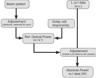
The procedure is described by the flow chart in figure 1: a far-field beam pattern characterization of the QCL allows us to determine, after corrections and adjustements, the optical power emitted for given temperature and driving current conditions. So, previously recorded relative L(I) data can be matched to this reference power to obtain absolute power vs current data.
L vs I data (a.u.)
Ref. Optical Power
(at I & T)
Absolute Power vs I data (W) Beam pattern
Adjustement
( treshold & sum) Golay cell responsivity
Adjustement
(match L(I) data to ref. power)
Fig. 1. Description of the method different steps
1) Beam pattern: The QCL is driven by a pulsed current
source, at 1.43A close to maximum power operation (pulse width = 40µs, duty cycle = 1%). Far-field beam pattern is acquired by moving in X and Y a Tydex GC-1T Golay cell whith an entrance aperture diameter restricted to 2 mm. The detector displacement is 82 mm x 82 mm with a 2mm scanning step and for each position, the average value and standard-deviation on 32 measurements are recorded. So, we obtain a 41x41 array representing the beam pattern.
Then, we calculate the beam centro¨ıd position whose horizon-tal and vertical coordinates, Hc and Vc, are given by:
Hc= ∑ (h× I(h, v)) I , Vc = ∑ (v× I(h, v)) I (1)
where I(h, v) is intensity at pixel (h, v) and I is the total intensity, integrated on the whole surface. Then, assuming that the beam is Gaussian, data from line and row passing at centro¨ıd are fitted to a Gaussian distribution in order to obtain horizontal and vertical beam widths at 1/e2. So, we
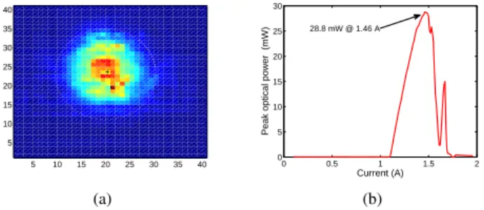
can define and plot an ellipse corresponding to the contour of the laser beam (fig. 2a). The sum of pixels inside the ellipse represents 86% of the total power.
2) Detector calibration: Previously, the Golay cell
respon-sivity was calibrated at 3.4 THz using a blackbody source at 373 K and a set of two filters (a 3.4 THz band-pass and a 10 THz low-pass) [3]. Regarding the slight difference between calibration and working frequencies compared to Golay cell operating range (∼ 37 GHz to 23 T Hz), we will consider, with a good approximation, detector responsivity at 3.8 THz equal to S = 28.2 kV.W−1 measured at 3.4 THz. 5 10 15 20 25 30 35 40 5 10 15 20 25 30 35 40 + (a) 0 0.5 1 1.5 2 0 5 10 15 20 25 30
Peak optical power (mW)
Current (A)
28.8 mW @ 1.46 A
(b)
Fig. 2. Beam pattern (+ is centro¨ıd position, dotted line shows ellipse
surroundings) and L(I) data
3) L(I) data recording: Light versus Intensity data were
recorded at the same temperature (4.2K) and under same driving conditions than for beam pattern acquisition. The Golay cell was just put in front of the cryostat window. An aperture diaphragm, inserted in the beam path just after the optical chopper, is used to limit the optical power reaching the detector in order to avoid saturation. The goal of this setup is only to record the shape of the L(I) curve.
B. Data corrections and final results
The sum Σ of pixels inside the ellipse is 3429 mV. The expression used to calculate the reference peak power is:
Pref = Σ× 1 S × 1 0.86× 1 DC × 1 τW × 4 π (2)
where S is the detector responsivity (in V/W), DC is the current pulses duty cycle, τ = 0.65 is the 3.5 mm thick cryostat window transmission coefficient at 3.8 THz. The constant factor 0.861 comes, as mentionned before, from the Gausian beam assumption and the factor π4 is used to correct the fact that, due to the detector circular aperture ϕ = 2mm
and the 2 mm scanning step, a part of the beam, propotional to the ratio beween the two corresponding surfaces.
So, we obtain a peak power value equal to 27.7 mW at 1.43 A. A coefficient is applied to previously recorded L(I) data to match the relative power at 1.43 A to 27.7 mW. At the end, we can plot the absolute peak power curve shown in figure 2(b) where the maximum peak power is 28.8 mW for 1.46 A injection current.
III. UNCERTAINTY ESTIMATION
From equation 2, the relative uncertainty on laser power can be written: ∆Pref Pref 2= ∆Σ Σ 2+ ∆S S 2+ ∆DC DC 2+ ∆τW τW 2 (3) The detector sensivity calibration was performed using a calibrated blackbody source and a band-pass filter. Due to non-linearities in the expression of power reaching the detector en-trance aperture, uncertainty cannot be calculated analytically. So, applying a random variation of all parameters (geometrical, temperature, atmospheric and filter transmission) numerical simulations were computed to determine a relative uncertainty ∆S
S = 11.7%. For the sum of pixels inside the beam ellipse,
the relative uncertainty ∆ΣΣ = 0.3% is estimated from the quadratic sum of errors at each pixel. Others contributions can be omitted because ∆DCDC = 0.1% and ∆ττ = 1%. Finally, the relative uncertainty on reference power is determined by responsivity: ∆Pref Pref = 11.7% IV. CONCLUSION
We have presented a simple and reliable method allowing the determination of absolute power emitted by THz sources such as Quantum Cascade Lasers. This method allows us to determine the optical power with a relative uncertainty close to 5.5% and was used for a 3.8 THz QCL which peak power was measured in the range (28.8 ± 3.4) mW , main contribution coming from the detector responsivity calibration.
ACKNOWLEDGMENT
The authors would like to thank Dr. Raffaele Colombelli from Institut d’Electronique Fondamentale (IEF) Orsay, Uni-versit´e Paris-Sud XI for providing the QCL.
REFERENCES
[1] L. Werner, H.-W. H¨ubers, P. Meindl, R. M¨uller, H. Richter, and A. Steiger, “Towards traceable radiometry in the terahertz region,” Metrologia, vol. 46, no. 4, p. S160, 2009.
[2] Y. Chassagneux, Q. Wang, S. Khanna, E. Strupiechonski, J. Coudevylle, E. Linfield, A. Davies, F. Capasso, M. Belkin, and R. Colombelli, “Limiting factors to the temperature performance of THz Quantum Cascade Lasers based on the resonant-phonon depopulation scheme,”
Terahertz Science and Technology, IEEE Transactions on, vol. 2, no. 1,
pp. 83–92, 2012.
[3] H. Kostkowski, Reliable spectroradiometry, S. consulting, Ed. La Plata, 1997.