To link to this article:
URL : https://www.jstage.jst.go.jp/article/isijinternational/51/2/51_2_242/_article This is an author-deposited version published in: http://oatao.univ-toulouse.fr/
Eprints ID: 5769
To cite this version:
Mendez, Susana and Lopez, David and Asenjo , Iker and Larranaga, Pello and Lacaze, Jacques Improved analytical method for chemical analysis of
cast irons. Application to castings with chunky graphite. (2010) ISIJ
International, vol. 51 (n° 2). pp. 242-249. ISSN 0915-1559
O
pen
A
rchive
T
oulouse
A
rchive
O
uverte (
OATAO
)
OATAO is an open access repository that collects the work of Toulouse researchers and makes it freely available over the web where possible.
Any correspondence concerning this service should be sent to the repository administrator: [email protected]
Improved analytical method for chemical analysis of cast irons.
Application to castings with chunky graphite.
Susana MENDEZ 1, David LOPEZ 1, Iker ASENJO 2, Pello LARRANAGA 2, Jacques LACAZE 3
1 - Chemical Department, AZTERLAN, Aliendalde auzunea 6, E-48200 Durango (Bizkaia), Spain
2 - Engineering and Foundry Department, AZTERLAN, Aliendalde auzunea 6, E-48200 Durango (Bizkaia), Spain 3 - CIRIMAT, Université de Toulouse, ENSIACET, BP 44362, 31030 Toulouse cedex 4, France
Abstract
Chunky graphite is a particular form of graphite degeneracy that appears in the centre of large iron castings, with a well-defined transition from the outer unaffected area and the inner affected one. All previous works that looked for macrosegration to explain the phenomenon concluded that there are no significant composition differences between the inner and outer parts of such castings. This was challenged again because the analytical methods generally used for chemical analysis are not efficient for low-level elements. Accordingly, an ICP-MS procedure has been developed and validated to replace the usual ICP-OES method. Together with the usual methods for analysis of C, S and Si, this ICP-MS procedure has been applied to characterize chemical heterogeneities in a large block with chunky graphite in its centre, and to a standard part for comparison. It could be concluded that no macrosegregation has built up during the solidification process of the block investigated,
i.e. that chunky graphite appearance is not related to any composition changes at the scale of
the cast parts, in particular of elements known to affect graphite shape such as Ce, Mg, Sb, S,…
Keywords
1.INTRODUCTION
Growth of graphite in nodular irons is often affected by degeneracy that leads to non spheroidal graphite precipitates 1). Amongst the various possibilities of graphite degeneracy,
chunky graphite (hereafter noted CHG) which consists of large cells of interconnected graphite strings 2, 3) often appears at the centre of heavy-section castings. At a micro-scale,
CHG cells appear as areas with small graphite precipitates as illustrated in Fig. 1. Such cells dramatically decrease the mechanical properties of the material, in particular fatigue properties for which such large parts have been designed. On a macro-scale, the area affected by CHG presents on a metallographic section a darker contrast than the fully nodular part of the casting, with a sharp transition between the non-affected and the affected zones. Because of the sharpness of this transition, a number of researchers have thought that this kind of graphite degeneracy should be related to some macrosegregation but failed to evidence it 4-6).
Preliminary measurements to the present study led to the same conclusion that the usual methodology used for chemical analysis does not allow evidencing any macrosegregation. Challenging this conclusion was the aim of the present work.
It is however known that chunky graphite formation is affected by the presence of low-level elements in the melt, though very little quantitative evidence of such effects has been given apart for Mg and Ce 7,8). Also, the interplay between the many impurities and
low-level elements has been scarcely looked for 9). Further, because of the duration of cooling
heavy-section castings, it seems reasonable that quite many complex chemical reactions take place during solidification of heavy-section cast-iron as suggested by Javaid and Loper 10).
These above observations suggested that differences in the composition of the metal should be studied at a scale close to the size of the CHG cells, i.e. a few mm3. This means that the
sampling size should be much smaller than the one used in previous studies and for usual chemical analyses which is typically 0.5 g, i.e. about 70 mm3. Such usual chemical analyses
are generally performed with an automatic combustion analyzer for C and S, by a gravimetric method for Si and by inductively coupled plasma optical emission spectroscopy (ICP-OES) for other elements.
While the quality of the determination is sufficient for C, Si and S, the quantification of low level elements (contents below 0.003 mass%) could be improved by using a more accurate analytical technique such as inductively coupled plasma mass spectroscopy (ICP-MS). Use of this technique is however limited due to lack of international standards that could certify concentration values lower than 0.003% with a guaranteed quality. This work was thus intended to develop chemical analyses with ICP-MS with appropriate quality for checking
macrosegregation of low level elements in heavy-section cast-iron castings. The whole process of setting-up analytical techniques, calibrating and measuring trace elements in small samples being about 0.1 g in weight is thus presented. Measurements of silicon, carbon and sulfur contents were performed with 0.5 g samples following the standard procedures that will be also shortly described for consistency. In the present work, these procedures have been applied to materials coming from the outer part (without CHG) and inner part (with CHG) of a heavy-section block. For purpose of comparison, measurements were also performed on material taken out from a light-section part that was cast with a melt of similar composition. This light-section part showed no CHG and presented a much larger nodule count.
Fig. 1 :
Optical micrograph showing cells of chunky graphite at the top right, top left end bottom right corners
2.EXPERIMENTAL DETAILS
The chemical analyses have been performed with three methods: -gravimetric method for silicon;
-combustion with a LECO CS-200 facility for carbon and sulfur;
-induction coupled plasma - mass spectroscopy (ICP-MS) with an Agilent 7500 CE apparatus for all other elements considered in this study.
The first and third methods apply to solutions obtained by dissolving the material in acids having ACS analytical grade, i.e. containing less than 5 ppm metal atoms. These three methods are successively detailed below with more detail for ICP-MS; they all give results per weight percents that are recalculated, either automatically or manually, from the initial masses of material involved for analysis which were weighed on calibrated balances with the following requirements:
-silicon analysis: 0.5 ± 0.005 g;
-carbon and sulfur analysis: 0.5 ± 0.005 g; -trace elements: 0.1 ± 0.0005 g.
2.1Measurement of silicon
Silicon is analysed along a procedure based on the E350 ASTM standard. The method consists in first dissolving the sample in a mixture of HNO3 (68 mass%) and HCl (38
mass%). Silicic acid H4SiO4 forms in the solution which is then dehydrated by fuming with
HClO4 leading to precipitation of silicon as SiO2. The solution is filtered, and the precipitated
silica and other compounds that were not soluble in acids (mainly graphite) are ignited together with the filter. The residues are weighed, and the silica present is then volatilized as SiF4 gas compound by adding hydrofluoric acid HF (48 mass%). The final residue is ignited
and weighed, the loss in weight representing volatilized silica and thus giving the initial silicon content in the material.
As the estimation of the silicon content is a gravimetric measure, it does not require calibration. Validation of the method was carried out using five certified international standards with silicon content cerw
Si in the range 0.25 to 3.17 mass%. For every selected
standard, the silicon content of ten samples weighting 0.5 g each was analyzed. This allowed characterizing the standard deviation of the procedure, σSi, and the difference from the
content has been calculated following the procedure detailed in annex 1, and its relation with the amount of silicon could be expressed as:
USi =0.0024 wSi + 0.0144 (mass%) (1) where wSi is the silicon content in mass%.
Further, a linear fitting (wSi=a cerwSi+b) of the Si contents estimated on the standard
samples could be expressed as:
wSi=0.9987 cerwSi - 0.0056 (mass%) (2)
with a regression coefficient of 0.9999. The uncertainties on the a and b coefficients were respectively 0.0063 and 0.0120 as estimated assuming that the errors in the measurements are independent and follow a Gaussian distribution. It is seen that the standard deviation on b is higher than its absolute value so that b could certainly be set equal to 0. Similarly, the standard deviation on a is high enough that a could certainly be assumed to be equal to 1. Because it is usual practice to express the results as given by least square fitting without any further analysis, no check of b equal to 0 and of a equal to 1 was however carried out. In the following of this paper, silicon contents will be expressed with at most the same number of digits as the standards used in the validation process (3 digits).
2.2Measurement of carbon and sulfur
C and S have been analyzed using an automatic analyzer LECO CS-200 that has two infrared (IR) cells dedicated the first one to S and the second to C. The sample is placed into a ceramic crucible together with an accelerator material, namely a commercial mixture of compounds, that decreases its melting point. The crucible is then positioned in the combustion chamber which is then purged and filled with pure oxygen. Finally, the furnace is turned on so that the sample burns within pure oxygen. During combustion, carbon atoms are oxidized to form mainly CO2 with some CO while sulfur atoms transform to SO2. After
combustion, the resulting atmosphere is swept to the analyzer by an argon carrier stream. S is measured as SO2 in the first IR cell of the analyzer. In between the two IR cells, the gas
passes firstly through a platinized silica gel catalyst at 355ºC in which the small amount of CO is converted to CO2 and SO2 is converted to SO3, and then through a cellulose filter that
Fig. 2 Schematic of the ICP-MS facility.
Calibration curves for C and S were obtained using eleven internationally certified standards with carbon contents varying from 0.014 to 4.11 mass% and sulfur contents from 0.0054 to 0.155 mass%. As already done for silicon, the measured weight content wi (mass%)
in element i (C or S) could be linearly fitted to the certified cerw
i value (mass%) and expressed
as:
wC=0.9897 cerwC+0.0047 with a regression coefficient of 0.9999 (3) wS=1.0242 cerwS-0.0007 with a regression coefficient of 0.9998 (3')
The uncertainties on the a and b coefficients were estimated and the same conclusions as before were reached.
Using the measurements on the certified standards, the uncertainties on the determination of C and S contents, UC and US respectively, have been calculated as detailed
in annex 1, and the relation with the amount of carbon or sulfur could be expressed as: UC =0.0116 wC + 0.0036 (mass%) (4)
where wC and wS are the carbon and sulfur contents (mass%). The contents in C and S will
finally be given with at most the same number of digits as the standards used to check the method, i.e. 3 digits for carbon and 4 digits for sulfur.
2.3ICP-MS
The content in every element other than Si, C and S was evaluated by ICP-MS from solutions prepared by dissolution in acid mixture consisting in HCl (38 mass%) and HNO3
(68 mass%). Distilled water of type I (according to the ASTM D1193 standard) was used for the dilution of samples and standards. Since spectroscopy is a comparative method, it needs a calibration step for which obtaining certified standard materials is difficult because usual standards do not reach the possible accuracy of ICP-MS. Synthetic samples were thus used instead of certified standards, they were prepared by appropriate additions of solutions of pure elements to the acid mixture.
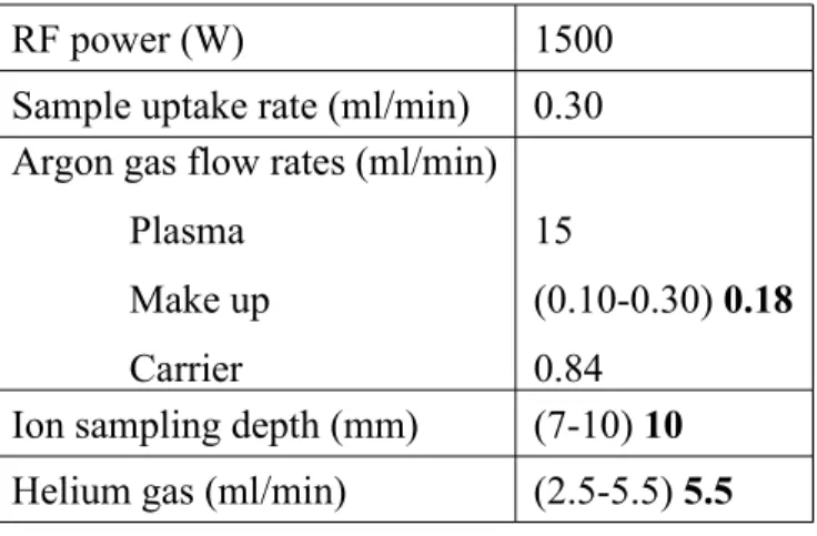
Table 1 – Standard ICP-MS operating conditions and optimum values (in bold) determined for three of them during the present work.
RF power (W) 1500
Sample uptake rate (ml/min) 0.30 Argon gas flow rates (ml/min)
Plasma Make up Carrier 15 (0.10-0.30) 0.18 0.84
Ion sampling depth (mm) (7-10) 10 Helium gas (ml/min) (2.5-5.5) 5.5
The ICP-MS instrument used is an Agilent 7500 CE schematically represented in Fig. 2 that is equipped with a facility for reaction and collision mode. Details of the instrument operating conditions and measurement parameters are reported in Table 1. In usual analysis conditions, the ICP-MS is used with parameters set at the values recommended by the manufacturer. However, a preliminary study was conducted to determine the range of values for three of these parameters with the aim at improving sensitivity and precision. These three parameters are the flow rate of the make-up gas (argon), the ion sample depth (distance between the torch and the sampling cone) and the flow rate of the reaction gas (helium). The
values of these three parameters can be changed from 0.10 to 0.30 ml/min for the flow rate of make-up gas, 7 to 10 mm for the ion sample depth, and 2.5 to 5.5 ml/min for the flow rate of the reaction gas.
Table 2
Isotopes selected for ICP-MS analyses, associated internal standard, regression coefficients (a and b) and regression factor R of the calibration curves, blank values (µg/l) and quantification limits (μg/l)
Element isotope Internal standard a b R Blank value Quantification limit 27Al 103Rh 4.548 10-3 2.425 10-3 0.9999 6.3 2 75As 103Rh 2.103 10-2 4.012 10-3 0.9999 0.95 2 137Ba 103Rh 4.504 10-2 2.661 10-3 1.0000 0.3 1 209Bi 205Tl 1.157 4.406 10-2 0.9999 0.0 1 140Ce 103Rh 1.048 -2.409 10-2 1.0000 <0.1 1 111Cd 103Rh 7.167 10-2 1.625 10-3 1.0000 <0.1 1 52Cr 45Sc 3.363 3.679 10-1 1.0000 1.0 7 63Cu 103Rh 2.369 10-1 1.313 10-1 0.9999 2.2 2 139La 103Rh 8.448 10-1 5.090 10-3 1.0000 <0.1 1 55Mn 45Sc 1.952 2.445 10-1 0.9999 15.0 2 26Mg 45Sc 4.129 10-2 6.051 10-3 0.9999 3.0 4 93Nb 103Rh 4.355 10-1 5.006 10-2 0.9997 0.2 1 146Nd 103Rh 2.143 10-1 -6.825 10-3 1.0000 <0.1 1 60Ni 45Sc 1.590 1.499 10-1 0.9999 13.7 4 208Pb 205Tl 1.409 1.058 10-1 0.9997 0.5 1 141Pr 103Rh 1.183 -1.127 10-2 1.0000 <0.1 1 121Sb 103Rh 9.966 10-2 1.333 10-2 0.9999 0.8 2 78Se 103Rh 1.971 10-3 6.178 10-4 0.9999 0.5 1 118Sn 103Rh 9.050 10-2 1.106 10-2 1.0000 0.7 2 125Te 103Rh 9.469 10-4 2.033 10-4 0.9989 0.7 1 49Ti 45Sc 7.694 10-2 6.292 10-3 1.0000 0.6 2 51V 45Sc 2.605 6.999 10-2 1.0000 0.5 1 89Y 103Rh 3.599 10-1 7.679 10-4 0.9999 <0.1 1 68Zn 103Rh 2.816 10-2 1.536 10-2 1.0000 7.4 3
This preliminary study was carried out with a solution containing 1 µg/l of three metallic elements with very different atomic masses Z: Co (Z=59), Y (Z=89) and Tl (Z=205). Ce (Z=140) was also added to monitor the level of polyatomic interferences because this species forms a strong oxide bond and has one of the highest oxide formation rate. Ce thus allows determining the proportion of double charges QCe2+/QCe+, with
(ZCe2+/QCe2+)/(ZCe+/QCe+)=70/140, and oxides CeO+/Ce+, with (ZCeO+/QCeO+)/(ZCe+/QCe+)=156/140,
that can be detected. The best conditions for use of the equipment are considered those that generate the highest counts for each of the elements with a small percentage of double charges and oxides detected by the relation Z/Q. The chosen values are indicated in bold font in table 1.
After checking possible interferences, the isotopes finally selected for analyses are indicated in table 2 which also lists of all the trace elements considered for this study. In most cases, the most abundant isotope was chosen, while in the case of Cd, Ni, Sn and Te the selected isotope was the one recommended by the manufacturer of the equipment for avoiding as much as possible interferences with other known masses. Other isotopes used in place of the most abundant ones had been selected for the following reasons:
26Mg: because the calibration curve obtained had better regression coefficient than the one
built with the most abundant isotope 24Mg;
78Se: to avoid the interference with Ar-Ar interactions at 80 atomic mass;
49Ti: because the calibration curve obtained had better regression coefficient than the one
built with the most abundant isotope 47Ti;
68Zn: to avoid interference with Ni at 64 atomic mass.
For the ICP-MS calibration a parent solution containing 1 mg/l of all the elements to be measured was prepared from 1.000 or 10.000 mg/l single-element solutions. From this parent solution, eight calibration standards were prepared with various concentrations in each of the elements (0.5, 1, 5, 10, 25, 50, 100 and 200 µg/l). In addition to the elements to be measured, each calibration standard contains also 10 μg/l of Rh, Sc and Tl, which will be used as internal standards, i.e. they will allow monitoring any loss of detection due to the process from the introduction of the sample in the ICP-MS instrument until the detection system. An internal standard is selected for every element to be analyzed (see table 2) and the count of the target ion (Yi) from the sample is divided by the ratio of the count (Ys) per
concentration (Cs) of the internal standard in the sample. The count value for every element
is thus a ratio:
Fig. 3 :
Examples of calibration curves for Cd, Mn and Cr. On the x-axis, the unit is ppb that corresponds to µg/l while y-axis gives the total count number obtained from
each solution sample.
Fig. 3 shows examples of calibration curves for Cd, Mn and Cr as the Y ratio of element i versus the i content of the standard stw
i. Regression analysis of the calibration
curves leads to express the ratio Ci as a linear function of stwi: Ci=a stwi+b. The values of the
a and b parameters for all analyzed elements, as well as the regression factor R, are listed in
Table 2. These regressions will serve to determine the concentration of an element in a sample by reading the counts from the solution in which it has been dissolved. The fact that the coefficients a and b vary from one elements to another is directly related to the ability of ionization of these elements and to the detection capability of the instrument. The coefficient a is directly linked to the transformation of the detected counts in concentration, while the coefficient b depends on the ionization and detection capabilities at low content in the element.
The ICP-MS results should thus be expressed as µg/l detected in the solution. Because of the very dilute solutions used in this method, a solution or sample with 1 μg/l is considered as equivalent to a solution with 1 µg/kg in weight. Further, as 0.1 g samples are dissolved in 100 ml of acid solution, detecting 1 µg/l in the solution corresponds to 1 µg/g (or 1 ppm) in the sample. Finally, since there are no certified standards for the very low contents of interest in this work, the results will be expressed in µg/g with one digit for values below 100 µg/g and no digit for values above 100 µg/g.
3.RESULTS
3.1Quantification limits and accuracy of the analysis procedure
For any types of analysis, the quality of the method should be first determined, this includes evaluation of the detection or quantification limits and of the accuracy. However, the quantification limits were not checked for C, S and Si because the lowest values to be analyzed in this work are always higher than the limits of the combustion and gravimetric methods (0.003 mass% S, 0.010 mass% C and 0.250 mass% Si). The accuracy was checked by performing a series of 10 independent measurements on each of the two standards BAS 481/1 and BAS 482-2.
Table 3 :
Content (mass%) in C, Si and S of the two standards (BAS 481/1 and BAS 482-2) as certified and as estimated in the present work. For each value, the uncertainty given by the manufacturer and the one evaluated from a series of ten measurements is also indicated
Standard Element Certified value Measured value BAS 481/1 C 3.907±0.009 3.912±0.048 Si 2.288±0.009 2.270±0.02 S 0.0040±0.0004 0.0038±0.0005 BAS 482-2 C 2.599±0.012 2.585±0.032 Si 1.815±0.007 1.820±0.02 S 0.0491±0.0015 0.0495±0.01
Table 3 compares the average value of these ten measures with the certified ones. The confidence interval of the experimental data at a level of 95% (i.e. calculated as indicated in annex 1) may also be compared to the confidence interval of the certified sample. In most cases, the difference between the average and certified values is less than 1% of this latter, except in the case of the low sulfur content of BAS 481/1 for which it amounts to 5%. The coefficient of variation of the experimental values, i.e. the ratio of the standard deviation to the mean values, is 0.5-0.6 % for C and Si while it is higher for S at 7% (BAS 481/1) and 20% (BAS 482-2). The above data show that the precision of the measurements as compared to the certified values is excellent for all three elements, being highly reproducible for C and Si and possibly more scattered for S.
For ICP-MS measurement, the limit of quantification of each element was determined by preparing a blank solution consisting in a mixture of a solution of pure iron (Sigma Aldrich 41305-4) and of the acids to be used to prepare the cast-iron samples. The purity of the iron is 99.999 mass% and the amount introduced in the blank corresponds to the amount to be found in the samples. Five independent analyses of the blank were then performed to look for any trace of every element of interest in this study that could have been introduced as impurity in the solutions or result from analytical biases. Using a generally accepted procedure, the quantification limit of the ICP-MS procedure for each element is then defined as ten times the standard deviation estimated from the five measures. Both blank values and detection limits thus determined are listed in table 2 where it is seen that the blank values are generally lower than the quantification limit, but for Al, Cu, Mn, Ni and Zn for which it is higher.
Three synthetic standards were then prepared to check the accuracy of the ICP-MS measurements. These standards consist in a iron-bearing mixture similar to the one prepared for the blank to which are made controlled additions of certified pure solutions of every trace element considered in this study. The three standards differ by the concentration in trace elements, namely 5, 20 and 50 μg/l. Five successive and independent ICP-MS measurements were performed on each standard solution that gave the mean values and uncertainties, Ui, are
Table 4 :
Mean value of five analyses and estimate of the uncertainty (Ui) on
ICP-MS measurements of standard solutions at 5, 20 and 50 µg/l. Uncertainty (Ui) estimated for ICP-OES measurements made on the 50
µg/l solutions are listed for comparison.
Element 5 µg/l standard 20 µg/l standard 50 µg/l standard
Mean Ui Mean Ui Mean Ui
Uifor ICP-OES 50 µg/l standard Al 7 1.9 24 4.2 58 8.7 16 As 5 0.6 22 2.0 52 3.1 16 Ba 5 0.9 21 1.6 53 2.9 --Bi 5 0.0 21 1.6 53 3.1 --Ce 5 0.1 20 1.0 52 2.1 15 Cd 5 0.1 20 0.8 50 0.9 --Cr 5 1.5 19 1.3 49 1.6 27 Cu 6 1.1 21 1.0 50 0.9 17 La 5 0.1 19 1.3 54 3.8 17 Mn 4 1.0 22 3.0 59 8.9 25 Mg 7 2.2 21 2.0 49 1.3 13 Nb 5 0.1 21 1.6 53 3.8 19 Nd 5 0.8 22 2.1 55 5.0 --Ni 6 1.1 21 1.6 54 4.2 2 Pb 7 2.0 22 1.8 51 1.4 17 Pr 5 0.1 20 1.3 51 2.7 --Sb 5 0.6 19 1.6 48 2.9 12 Se 5 0.8 20 1.4 52 2.0 --Sn 5 0.8 19 1.6 48 2.9 7 Te 5 0.9 19 0.9 49 1.3 --Ti 5 0.9 20 1.2 50 0.8 27 V 5 0.5 19 1.3 48 2.6 4 Y 6 0.9 22 2.1 57 6.5 --Zn 16 11 32 11.6 61 11.4 18
For most elements, it is seen in table 4 that all ICP-MS measurements gave mean values differing from either 5, 20 or 50 µg/l values by less than the corresponding Ui value. It
is noteworthy also that the Ui values are most often less than 1, 2 and 5 for the 5, 20 and 50
µg/l solutions respectively, i.e. correspond to a precision better than 20%, 10% and 10% respectively. Exceptions to this latter observation are Al, Mn and Zn that show much higher Ui values; this may be somehow related to the fact that they showed also high blank values
(see table 2) but such an hypothetical relation was not investigated further.
Finally, the Ui values associated with ICP-OES measurements are also listed in Table 4, but only for the 50 µg/l solutions as the quantification limit of this method is larger than 20 µg/l for most elements. It is seen that the Ui values are generally much lower for ICP-MS than
for ICP-OES, this former method improving the sensitivity by more than one order of magnitude for some of the studied elements.
3.2Cast-iron samples
As indicated in the introduction, three metal pieces were analyzed. The first two pieces were machined out from a large cubic block (0.3 m in size) as thin slices about 0.3 mm in thickness, one from the centre where a high fraction of chunky graphite was observed (labeled CHG) and the other from the outer part of the block that was free of chunky graphite (labeled no-CHG). The third piece was taken out from a standard light-section foundry part (0.01 m section thickness) which had a composition similar to that of the block and was intended for comparison purpose (labeled SGI). Both castings were made in sand mold using standard foundry practice as described elsewhere 11). From each slice, ten little 0.1 g samples
were cut out for ICP-MS, two 0.5 g samples for C and S and one 0.5 g sample for Si analyses. In the case of the CHG material, observation of both surfaces of the slices allowed selecting samples in which most of the graphite was chunky.
C and S were analyzed twice, with the requirement that the two values did not differ by more than 0.05 mass% for carbon and 0.002 mass% for sulfur. If this requirement was not fulfilled the equipment was checked and the sample preparation and analysis were performed again. It may be mentioned that differences between the two carbon analyses may be due to a lack of homogeneity among the samples but also to graphite particles dropping out from the sample surface during slicing and adjusting sample weight. The ten samples of 0.1 g were successively dissolved in 10 ml of a mixture of acids (three parts HCl and one part HNO3) in
Teflon vessels on a hot plate at 250°C. After dissolution, the liquid was filtered using a medium porosity (20-25 µm) paper and diluted with distilled water to obtain 100 ml of solution. Whenever the concentration of an element was found higher than the highest range
of the calibration curve, the measurement was carried out again after one further dilution (1:100) from the initial preparation. This was indeed the case of Mg, Cr, Mn and Ni.
The average values mi,the standard deviation σi and the uncertainty Ui are listed in
table 5 for all the analyzed elements i. It is seen in this table that the standard deviation σi
was zero or undetermined for some elements that are present at very low level (Ba, Bi, Cd, Nd, Pr, Se, Te and Y). In addition, it is noted that the calculated uncertainty is higher than 50% of the estimated content in the case of Pb. This means that very low levels can not be measured quantitatively by this method, the minimum concentration for such analysis being estimated at 5 µg/g. Because of that, the nine very low level elements above will not be considered any further.
It is seen in Table 5 that the measurements on the block are quite scattered, most of the standard deviations amounting to more than 10% of the corresponding average value, with the exception of C and Si. On the contrary, the measurements on the standard SGI part show much higher reproducibility. This difference is illustrated by the graphs in Figure 4 that compare the individual measurements series for some of the elements: i) Ce, Mg and Sb that are known to affect graphite shape; ii) Cu and Zn that showed values differing in the CHG and no-CHG zones (see below); and iii) C and Si as main elements. This scattering in the results on the material taken out from the block is certainly due to its coarser solidification structure, with less and larger nodules than in the reference SGI part. Picking up small pieces 0.1 g in weight thus added a microstructure component to the composition variations that is much less pronounced with the finer structure of the SGI part.
It is of interest to note that comparing in Fig. 4 the range and scatter of the elements affecting graphite shape, Ce, Mg and Sb, does not allow drawing any relation with the presence of chunky graphite. For a more quantitative comparison, the difference between average species contents in CHG and no-CHG areas was compared to the sum of their associated uncertainties. A difference higher (resp. lower) than this sum would correspond to a change (resp. no change) in the content of the corresponding element. As a matter of fact, it was found that the contents in nine elements (Al, As, La, Mn, Mg, Ni, Sb, Sn and S) do not show any variation between the CHG and no-CHG areas. The contents in the remaining seven low level elements (Ce, Cr, Cu, Nb, Ti, V and Zn) showed all a decreased from the no-CHG to the no-CHG areas, with the exception of Cu content that increased. Finally, it may be observed an increase in both C and Si from the no-CHG to the CHG areas.
Table 5 :
Average of ten measures, standard deviation and uncertainty U (µg/g, except for C, S and Si that are given in mass%). n.d.: not determined
Element no-CHG CHG SGI Mean value Standard deviation Ui Mean value Standard deviation Ui Mean value Standard deviation Ui Al 102 10.9 14 115.9 9.9 16 66.2 3.0 9.7 As 7.8 1.2 1.0 6.6 1.4 0.9 13.6 0.5 1.3 Ba 1 0 0.7 1 0 0.7 2.5 0.5 0.7 Bi <1 n.d n.d <1 n.d n.d <1 n.d n.d Ce 39.2 12.7 1.6 30.9 13.5 1.3 19.2 0.9 0.8 Cd <1 n.d n.d <1 n.d n.d <1 n.d n.d Cr 357 38 2.5 320 50.1 2.3 28.9 8.8 1.4 Cu 59.6 26.3 0.8 127.2 8.2 0.5 26.9 5.3 1.0 La 19.5 3.5 1.3 17.7 2.9 1.1 10.1 0.6 0.6 Mn 950 67.5 138 883 86.2 129 2626 226 383 Mg 360 50.1 16 335 70.7 17 202 4.2 20 Nb 15.9 4.2 1.1 11.6 4.8 0.7 15.9 4.2 1.1 Nd <1 n.d n.d <1 n.d n.d <1 n.d n.d Ni 216 25.9 15 217 19.5 15 211 9.9 15 Pb 3.0 3.9 2.0 1.5 1.1 2.0 2.9 1.2 2.0 Pr <1 n.d n.d <1 n.d n.d <1 n.d n.d Sb 3.4 0.7 0.6 3.0 0.5 0.6 6.0 0 0.8 Se <1 n.d n.d <1 n.d n.d <1 n.d n.d Sn 12.1 1.3 1.2 10.9 1.4 1.2 27.7 0.8 2.0 Te <1 n.d n.d <1 n.d n.d <1 n.d n.d Ti 59.9 20.2 0.9 40.6 21.7 0.9 12.5 1.8 1.0 V 78 13.1 4.2 63 16.8 3.4 26.1 0.9 1.6 Y <1 n.d n.d <1 n.d n.d <1 n.d n.d Zn 115.9 8.4 12 43.8 15.1 11 982 23.0 18 C 3.63 0.03 0.04 3.73 0.03 0.05 3.62 0.01 0.04 S 0.0113 0.0007 0.0007 0.0100 0.0011 0.0007 0.0132 0.0004 0.0008 Si 2.09 0.01 0.02 2.15 0.09 0.02 2.19 0.03 0.02
Figure 4 :
Plot and comparison of measurements made on the three cast iron samples, labeled no-CHG, CHG and SGI. The plots are for selected elements only,
It would appear at first difficult to decide if any macrosegregation may or not be associated with the appearance of CHG as there are 9 elements that do not show compositional change and nine others that do so. However, the higher C and Si values found in the CHG zone could easily be related to the fact that the samples were preferentially collected from zones with high amount of chunky graphite. Accordingly, the average carbon equivalent of the no-CHG areas calculated as wC+0.28wSi 12) is slightly hypoeutectic at 4.22
mass% while that for the CHG areas is eutectic at 4.33 mass%, in agreement with the often assumed eutectic nature of the CHG cells. The difference in carbon and silicon contents may thus be due to the selection of the samples in the case of the CHG areas and not to a change in the overall composition of the material. It is known that Cu segregates negatively as does silicon, i.e. with a partition coefficient between austenite and liquid higher than 1. Accordingly, the higher Cu value in the CHG zone than in the no-CHG zone shows the same trend than for Si and might thus be associated also to eutectic growth. For all other elements that show a decrease, an opposite redistribution behavior may be expected with a partition coefficient between austenite and liquid lower than 1. Accordingly, that elements did not show significant changes from the no-CHG to the CHG areas may be related to high uncertainties associated to their estimation. To sum-up, the present results suggest that the changes observed in the content of half of the estimated species are associated to the selection of the samples in the CHG area. This conclusion allow excluding that any macrosegregation had built up during solidification of the block.
It seemed of interest to compare the results of the present work to those reported in the literature 4-6). For that purpose, the composition differences ∆ between CHG and no-CHG
areas have been plotted in Figure 5 where only elements that have been measured in at least two of these four works have been considered. For four elements, namely Bi, Ce, Mo and V, there is anyway only one bar appearing in the figure, and this means that the other reported differences were zero. It is noteworthy that ∆ is negative for all measurements reported for Cr and Sn, and positive for all Cu and Ni measurements. This is tentatively related to the eutectic nature of CHG cells as discussed above. For all other elements, the behavior of ∆ seems erratic with either positive or negative values, so that no correlation can be established between composition change and CHG appearance, in particular in elements that are known to affect graphite shape. The observation of Fig. 5 is thus in line with the previous conclusion that no macrosegregation could be associated with CHG areas.
Figure 5 :
Difference between compositions measured in CHG and no-CHG zones according to the present work and literature.
4. CONCLUSIONS
An MS procedure has been developed and validated to replace the usual ICP-OES method for measuring low level elements in cast irons with the aim at decreasing the quantification limits. The validation of the methods has been carried out and it has been shown that ICP-MS presents accuracy and uncertainty values much better than those for the most used ICP-OES method, with in some cases an improvement by more than one order of magnitude. Together with the usual combustion analysis for C and S and gravimetric method for Si, this ICP-MS procedure has been used to look for any macrosegregation related to the formation of chunky graphite in heavy-section ductile iron castings.
No statistically significant differences could be found between areas with and without CHG for half of the measured elements, including Mg, S and Sb that are known to affect graphite shape. Slight differences were found for the other half, including C and Si. On the
basis of the contents in these two latter elements, the observed differences could be related to the preferential collection of the samples in the CHG areas where pieces with highest amounts of eutectic CHG cells were selected. These results suggest that no macrosegregation did built during solidification of the heavy-section casting analyzed that could explain chunky graphite appearance. Research is going on to look for an evolution of the local distribution of those elements without composition change, e.g. by precipitation of oxides or compounds in which low level elements could be tight and thus no more available for the control of graphite shape.
R
EFERENCES1)R. Elliott: Cast iron Technology, Butterworths, London, (1988).
2)P.C. Liu, C.L. Li, D.H. Wu and C.R. Loper: Trans. AFS, 91(1983), 119.
3)T. C. Xi, J. Fargues, M. Hecht and J.C. Margerie: Proc. of Mat. Res. Soc. Symp., H.
Fredriksson and M. Hillert eds., Elsevier Science Publishing Co., North-Holland, New-York, USA, 34(1985), 67.
4)M. Gagné and D. Argo: Proc. of Advanced Casting Technology, Easwaren J. ed., ASM Int.,
Metals Park, Ohio, USA, (1987), 231.
5)B. Prinz, K.J. Reifferscheid, T. Schulze, R. Döpp and E. Schürmann: Giessereiforschung
43(1991), 107.
6)R. Källbom, K. Hamberg. and L.E. Björkegren: Proc. of 67th World Foundry Congress,
Harrogate, UK, (2006), paper 184.
7)O. Tsumura, Y. Ichinomiya, H. Narita, T. Miyamoto and T. Takenouchi: IMONO, 67(1995), 540.
8)P. Larranaga, I. Asenjo, J. Sertucha, R. Suarez, I. Ferrer and J. Lacaze: Metall. Mater.
Trans.A, 40A(2009), 654.
9)H. Löblich: Giesserei, 93(2006), 28.
10)A. Javaid and C.R. Loper: Trans. AFS, 103(1995), 135.
11)I. Asenjo, P. Larranaga, J. Sertucha, R. Suarez, J.-M. Gomez, I. Ferrer and J. Lacaze: Int. J. Cast Metals Res., 20(2007), 319.
12)M. Castro, M. Herrera, M.M. Cisneros, G. Lesoult, J. Lacaze: Int. J. Cast Metals Res.,
Annex 1
The calculation of the uncertainty associated with chemical analysis of the content in i species of a sample is based on the series of measurements made on certified materials and on the sample itself. It is expressed as the square root of the variance related to the measures which comes from three sources:
-the possible error on the standard composition in element i, Ui,0, indicated by the
manufacturer;
-the possible errors induced by the analytical method due to the determination of the mean
value from a limited number of measurements. If σi,m and nc are the standard deviation and
number of measurements made on the standard, and σi,a and n those for the sample, the
respective uncertainties are
c n m ,i m ,i U = σ and n a ,i a ,i U =σ ,
-from a possible bias associated to the analytical method that leads to a systematic difference between the measured, wi, and certified, cerwi, values, ∆wi=cerwi-wi. The bias may be estimated
by a large enough number of measurements (in practice 10 in the present work) on the standard.
All measurements should be made fulfilling the maximum of the reproducibility conditions defined by the ASTM E-177 standard as conditions where the results are obtained with the same method on identical test items (or taken at random from a single quantity of material that is as homogeneous as possible) in different laboratories with different operators using different equipment. These conditions were satisfied in the present case apart for the fact that all measurements were made in the same laboratory.
Assuming that the variance associated to the analytical method is the same for the standards and the samples, one has σi= σi,m=σi,a. Assuming the three sources of errors are
independent, and that the one associated to the analytical method follows a Gaussian law, the variance of one measure is the sum of the three variances listed above. The uncertainty Ui on
the content in species i is finally given as:
2 2 2 2 0 , 1 1 i c i i i w n n K U U + ∆ + + = σ
The uncertainty on each element is always calculated from certified standards at least at three levels of composition (low, medium and high values) so as to span the range of possible measurements. The uncertainty Ui for any other value in the measuring range is then
determined by a linear fit of the values determined on the standards, i.e. Ui = a wi + b where a