Spectral analysis of unsteady flow simulation in a small VAWT

(1)

Science Arts & Métiers (SAM)

is an open access repository that collects the work of Arts et Métiers Institute of Technology researchers and makes it freely available over the web where possible.

This is an author-deposited version published in: https://sam.ensam.eu Handle ID: .http://hdl.handle.net/10985/6731

To cite this version :

Annie-Claude BAYEUL-LAINE, Sophie SIMONET, Gérard BOIS - Spectral analysis of unsteady flow simulation in a small VAWT - In: 14th International Symposium on Transport Phenomena and Dynamics of Rotating Machinery, ISROMAC-14, United States, 2012-02 - ISROMAC-14 - 2012

Any correspondence concerning this service should be sent to the repository Administrator : archiveouverte@ensam.eu

(2)

1 14th International Symposium on Transport Phenomena and Dynamics of Rotating Machinery, ISROMAC-14 February 27th - March 2nd, 2012, Honolulu, HI, USA

Annie-Claude BAYEUL-LAINÉ

1

*, Sophie SIMONET

1

, Gérard BOIS

1

LML, UMR CNRS 8107, Arts et Metiers PARISTECH,

8, boulevard Louis XIV 59046 LILLE Cedex, FRANCE

annie-claude.bayeul@ensam.eu

Abstract

The vertical axis wind turbine studied in this paper combine two rotations: one rotating movement of each blade around its own axis and one rotating movement around turbine’s axis.

The aim of this paper is to analyse the effect of this two combine movements on fields of pressure and on global forces on each blade with time. Preliminary calculations showed, for some initial blade stagger angles (angle between blade 1 and x axis), that flow is highly unsteady and sometimes hardly periodic.

The main goal here is to present spectral analysis of unsteady results like temporal pressure on specific points in the domain and temporal forces on blades and to show the influence of the two combine movements for two different blade stagger angles for elliptic blades.

.

Keywords:

Numerical simulations, performance coefficient, unsteady simulation, VAWT, vertical axis, wind

energy, pitch controlled blades. Nomenclature

Cp power coefficient (no units)

Ceff real torque (mN/m)

D diameter of turbine zone (m) EB elliptic blades

f frequency (Hz)

f* non dimensional frequency fz blade passing frequency (Hz)

fzi blade passing frequency’s harmonic (Hz)

Gi center of rotation of blade i

L length of blade (m) Lp pressure level (dB)

Mti torque of blade i by turbine axis, (mN/m)

O center of rotation of turbine in 2D model Peff real power

R radius of axis of blades, =0.62 m

Re Reynolds number based on length of blade

Rt radius of blade tip, m

S captured swept area, m2 SB straight blades

V0 wind velocity, =8 m/s

Z number of blades (Z=3)  blade stagger angle (degrees)

  blade or tip blade speed ratio (no units)

 density of air, kg/m3

 azimuth angle of blade 1(degrees)

1 angular velocity of turbine (rad/s)

2 angular velocity of pales (rad/s)

Subscripts i blade index 1 Introduction

All wind turbines can be classified in two great families (Leconte P., Rapin M., Szechenyi E. (2001[10]), Martin J. (1987) [11]) (i) horizontal-axis wind turbine (HAWTs) and (ii) vertical-axis wind turbine (VAWTs). Figure 1 shows typical power coefficient of several main types of wind turbine. VAWTs work at low speed ratios.

A lot of works was published on VAWTs like Savonius or Darrieus rotors (Hau E.(2000[9]), Paraschiviou I. (2002 [13]), Pawsey N. C. K. (2002 [14])…) but few works were published on VAWTs with relative rotating blades (Bayeul-Lainé A.C. and al (2010, 2011 [2-4]), Cooper P. (2005, 2010 [5-6]), Dieudonné P. A. M.(2006 [7])). Some inventors discovered this kind of turbine in the same time on different places (Cooper P., Dieudonné

(3)

2 P.A.M. for example) and made studies these last ten years

on this kind of VAWTs.

Fig. 1 Aerodynamic efficiencies of common types of

wind turbines from Hau (2000)

In 2008, F. Penet, P. de Bodinat and J. Valette gained an innovation price for an idea in which this kind of turbine is used to make a publicity panel lighted by wind energy. They created the society Windisplay to design, create and send such a product. The present study concerns this kind of VAWT technology in which each blade combines a rotating movement around its own axis and a rotating movement around turbine’s axis. It is an extensive study of a work given by this young people. This paper concerns the industrial one.

The aim of previous studies presented in 2010 (Bayeul-Lainé A.C. and al [2-3]) was to give some numerical results like contours of pressure, velocity fields and power coefficients, compared to relative steady blades for a blade speed ratio of 0.4, a wind velocity of 8 m/s and for four blade stagger angles. The commercial code Star CCM+ 5.02.010 was used to make calculations. The benefit of rotating elliptic blades was shown: the performance of this kind of turbine was very good and better than those of classical VAWTs for some specific initial blade stagger angles between 0 and 15 degrees. It was shown that each blade’s behaviour has less influence on flow stream around next blade and on power performance. The maximum mean numerical coefficient was about 32%.

Results were also compared to some other numerical results. The blade sketch needs to have two symmetrical planes because the leading edge becomes the trailing edge

when each blade rotates once time around the turbine’s axis.

New simulations were performed with straight blades in 2011 [4]. Results were compared between elliptic blades and straight blades: local results like contours of pressure, velocity fields, unsteady power coefficient, mean power coefficient.

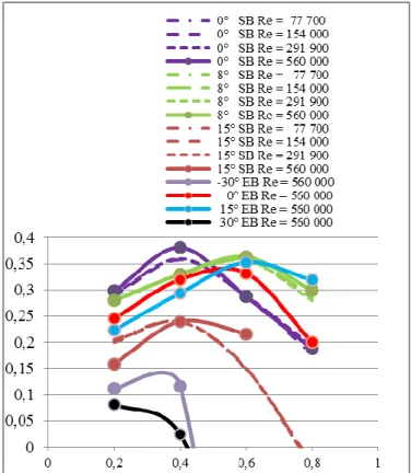
Fig. 2 Mean power coefficients for all test cases with

blade speed ratios  The following conclusions have been drawn:

- The performance of this kind of turbine was confirmed to be very good and better than those of classical VAWTs for some specific blade stagger. The maximum mean numerical coefficient at a blade speed ratio equal to 0.4 was about 38% (Fig. 2).

- Each blade’s behaviour seems to have less influence on flow stream around next blade and on power performance. - A significant influence of sketch of blades depending on other parameters like blade speed ratios and initial blade stagger angles.

- A significant influence of blade speed ratios

- A significant influence of initial blade stagger angle - A low influence of Reynolds number

- A better stability of results for elliptic profiles

A wide range of results have been obtained and still needs more analyses to understand all what happens in this VAWT. A lot of work has still to be done: influence of

(4)

3 number and relative position (radius of centre) of blades,

analytical analysis, spectral analysis…

This paper deals with the spectral analysis of unsteady results like temporal pressure on specific points in the domain and temporal forces on blades for elliptic blades, a wind velocity of 8 m/s for two specific cases:

- Case a : blade speed ratio  equal to 0.6, initial blade stagger angle equal to 15 degrees which gives one of the best mean power coefficient and a relative periodicity for temporal forces

- Case b : blade speed ratio  equal to 0.2, initial blade stagger angle equal to 30 degrees which shows a high unsteady flow

2 Non dimensional coefficients

The common non dimensional coefficients used for all wind turbines are:

- Efficiency of a rotor, named power coefficient

2 V S P C ₃ 0 eff p   ₍₁₎

In which Peff is the power captured by the turbine and 2

V S ₀3



is the total kinetic energy passing through the swept area (Fig. 3).

- Speed ratio 0 t V R    ₍₂₎

Where the angular velocity of the turbine is, R_t is generally the radius blade tip (radius of center of blade in case of this paper) and V0 the wind velocity.

- Reynolds number Re (Marchaj C. A. [15]) based on blade’s length

  V L

Re 0 (3)

3 Geometry and test cases

The sketch of the industrial product is shown in Figure 3. Blades have elliptic sketches, relatively height, so a 2D model was chosen. The calculation domain around turbine is large enough to avoid perturbations as showing in Figure 4. Elliptic blades have minor radius of 75 mm and major radius of 525mm. Distance between turbine axis and blade axis is 620 mm.

The mesh (Fig. 4,5) was refined near interfaces. Prism layer thickness was used around blades. The resulting computational grid is an unstructured triangular grid of about 60 000 cells.

A time step corresponding to a rotation of 1/2048 revolution was chosen in view of spectral. So a new mesh was calculated at each time step.

Fig. 3 Sketch of the VAWT studied

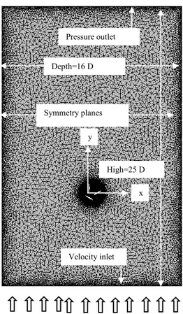
Fig. 4 Mesh and boundaries’ conditions

Boundary conditions are velocity inlet to simulate a wind velocity in the lower line of the model (Re=560 000),

symmetry planes for right and left lines of the domain and pressure outlet for the upper line of the domain. The model contains five zones: outside zone of turbine, three blades zones and zone between outside zone and blades zones named turbine zone. Turbine zone has a diameter named D (equal to the sum of R, plus the major radius of blade plus a little gap allowing grid mesh to slide between

Velocity inlet Symmetry planes Depth=16 D Pressure outlet High=25 D x y

(5)

4 each zone). Except outside zone, all other zones have

relatively movements. Four interfaces between zones were created: an interface zone between outside and turbine zone and an interface between each blade and turbine zone. Details of zones are given in Figure 5.

Fig. 5 Zoom of the mesh of the VAWT studied

The vertical axis wind turbine studied in this paper combine two rotations: one rotating movement of each blade around its own axis and one rotating movement around turbine’s axis as we can see in figure 5.

4 Torques and power coefficients

For this kind of turbine each blade needs energy to rotate around its own axe so real power captured by the turbine has to be corrected.

Code gives torque Mt around turbine axis for each blade, pressure forces and viscosity forces.



    i blade S i i blade S i ti OG df G M df M     (4) O is the turbine centre, Gi is the axis centre of blade i and

d

f



is elementary force on the blade i due to pressure and viscosity, so i 2 i 1 ti C C M   (5)



   i blade S i 1 i 1 C bladei OG df C   (6)



   i blade S i 2 i 2 C bladei GM df C   (7) Real power was given by:



      3 , 2 , 1 i i1,2,3 2 i 2 1 ti eff M C P (8)

with 1, angular velocity of turbine and 2 relative angular velocity of each blade around its own axis. As

2 1 2   (9)







    3 , 2 , 1 i 1 i 1 ti eff 2 C M P ₍₁₀₎

And power coefficient is given by equation (1) in which swept area is those showed in figure 3 for the cases with three rotating blades

5 Results

5.1 Temporal results

Fig. 6 Pressure probes

Probes p1 p2 p3 p4 p5 p6

x (m) 0.4 0.6 0.8 1.0 1.2 1.4

y (m) 1.2 1.2 1.2 1.2 1.2 1.2

Table 1 Pressure probes position

Instantaneous torques, Fpx, Fpy and pressure probes are given in figures 7 to 14 for each case. In order to explain the choice of these two cases, it seems interesting to examine these instantaneous global results. For the case a, a good periodicity corresponding to the rotation of each blade can be observed. On the contrary highly instabilities appear for the case b.

To understand these behaviours, the contours of relative pressure are given in figures 15 to 22. For each kind of blades, a swirl arises at the leading edge of the lower blade. This swirl grows up when the blade rotates and breaks off blade for some azimuth angle, and then it reduces until vanished. This can be observed more accurately for an initial blade stagger angle of 15 degrees. These results are backed up by the examination of Z-vorticity in figures 23 to 30. Moreover, the examination of these figures point up negative vorticities in the wake of blades, probably due to the rotation of blades around their own axes. This was detected only by Z-vorticity results.

Outside zone Turbine zone

Blade 2 zone

Blade 1 zone

Blade 3 zone

(6)

5

Case a: initial blade stagger angle 15 degrees Blade speed ratio 0,6

Fig. 7 Torques with azimuth angle of blade 1 (mN)

Fig. 8 Fpx with azimuth angle of blade 1 (mN)

Fig. 9 Fpy with azimuth angle of blade 1 (mN)

Fig. 10 pressure with azimuth angle of blade 1 (mN)

Case b: initial blade stagger angle 30 degrees Blade speed ratio 0,2

Fig. 11 Torques with azimuth angle of blade 1 (mN)

Fig. 12 Fpx with azimuth angle of blade 1 (mN)

Fig. 13 Fpy with azimuth angle of blade 1 (mN)

(7)

6

Fig. 15 Contours of pressure for=0 degree

Fig. 16 Contours of pressure for=30 degrees

Fig. 17 Contours of pressure for =60 degrees

Fig. 18 Contours of pressure for =90 degrees

Fig. 19 Contours of pressure for=0 degree

Fig. 20 Contours of pressure for=30 degrees

Fig. 21 Contours of pressure for =60 degrees

(8)

7

Fig. 23 Z-vorticity for=0 degree

Fig. 24 Z-vorticity for=30 degrees

Fig. 25 Z-vorticity for =60 degrees

Fig. 18 Z-vorticity for =90 degrees

Fig. 27 Z-vorticity for=0 degree

Fig. 28 Z-vorticity for=30 degrees

Fig. 29 Z-vorticity for =60 degrees

(9)

8 In view to understand the birth of this swirl, some

pressure probes were created (Fig.6, Table 1). The temporal results are presented in figures 10 and 14 and spectral analyses of these results are done hereafter. 5.1 Spectral analysis

The spectral analysis is performed on the pressure results given by the probes P1 to P6 (position defined in figure 6 and on table 1) for the both cases; case a for convenient performances and case b for degraded performances of the VAWT.

As the two cases have different rotation speeds, the results are plotted in function of the non-dimensional frequency f* which is defined by equation (11).

(11)

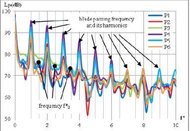
fZ is the blade passing frequency, given by equation (12). (12) The temporal results are treated with a Fast Fourier Transform (FFT).The FFT calculations are performed in terms of pressure level (in dB, with a reference pressure p0 equal to 2 10-5 Pa)

Fig. 31: pressure level for Case a, initial blade

stagger angle 15 degrees, blade speed ratio 0,6

The results presented in figure 31 show that the periodicity of the pressure is well established, particularly for the probes 3-4-5.

It can be noticed that the probe 6 presents less amplitude than the other, perhaps due to the fact that the other blades influence the signal and hide the perturbations of the pressure field which is seen by this probe. This is

convenient with the amplitude shown on the time dependent signal in figure 10.

For some probes, other frequencies, different of the blade passing frequency and its harmonics, appears. These frequencies are linked to the two different rotational speeds 1 and 2. In figure 31, it is indicated that there are phenomenon appearing at f2i* defined by equation

(13). The factor 1/2 comes from the relation between the angular velocity of the turbine 1 and the angular velocity

of the blade 2 (eq.9).

(13) There is also a perturbation for f* equal to 4.5 which is perhaps also due to the combine movements of blades and turbine.

Fig 32. : Evolution of the torque in case a.

Fig. 33: Comparison of pressure level between case a and

(10)

9 As can be observed in figure 32, the periodic effect for

the torque disappears quickly. Only the two first frequencies can be observed accurately. This is in good agreement with the good performances of the turbine in this configuration.

The comparison between the two cases shows important differences (fig.33). The periodicity doesn’t appear in the case b. The pressure level for case b is higher of 10 dB than the pressure level for case a, except at the blade passing frequency and its harmonics; this can be explained by the fact that there are more instabilities in the flow field for the case b.

6 Conclusion

Comparison between two cases was performed in this study (i) case a with blade speed ratio  equal to 0.6, initial blade stagger angle equal to 15 degrees (ii) case b with blade speed ratio  equal to 0.2, initial blade stagger angle equal to 30 degrees which shows a high unsteady flow.

In the two cases, it has been shown that a swirl arises from the leading edge of the first blade near the wind then grows up when the blade rotates until it vanishes when the trailing edge becomes trailing edge (pressure contours and Z-vorticities). The effect of this swirl was also captured by the pressure probes.

The examination of Z-vorticity points up swirls with negative magnitude in the wake of blades, probably due to the double rotations of blades.

The spectral analysis performed on pressure results with FFT calculation, shows that the periodicity of the pressure is well established, especially for the probes 3-4-5 in case a. For some probes, other frequencies, different of the blade passing frequency and its harmonics, appears for case a. These frequencies are linked to the two different rotational speeds 1 and 2. On the contrary, for case b, the periodicity hardly appears. The comparison between the two cases shows a high difference of 10dB between pressure levels.

It will be interesting in the future to study the noise generated in the far field. The pressure level, represented in figure 33, suggests that for case a, the perturbation will give dipole source (due to aerodynamics forces fluctuations) and that for case b it will leads to quadrupole source (due to turbulence) as can be predicted using the Ffowcs-williams and Hawkings analogy [8] and as can be observed for other turbomachines [11].

References

[1] Abbott I. H. , Von Doenhof f A. E., 1949, Theory of wing sections, Mc Graw Hill Book, ISBN 486-60586-8 [2] Bayeul-Lainé A. C., Bois G., Simonet S., 2010, « Etude numérique instationnaire d’une micro-éolienne à axe vertical », 1ère Conférence Fanco syrienne sur les énergies renouvelables, octobre , Damas, Syrie

[3] Bayeul-Lainé A.C., Bois G., 2010, « Unsteady simulation of flow in micro vertical axis wind turbine », Proceedings of 21st International Symposium on Transport Phenomena, Kaohsiung City Taiwan, 02-05 november,

[4] Bayeul-Lainé A. C., Dockter A., Bois G., Simonet S., 2011 , “Numerical simulation in vertical wind axis turbine with pitch controlled blades”, IC-EpsMsO, 4th , Athens, Greece, 6-9 July, pp 429-436

ISBN 978-960-98941-7-3

[5] Cooper P., Kennedy 0., 2005, “Development and analysis of a novel Vertical Axis Wind Turbine”,

http://www.datataker.com/public_domain/PD71%20Deve lopment%20and%20analysis%20of%20a%20novel%20v ertical%20axis%20wind%20turbine.pdf

[6] Cooper P. (2010), Wind Power Generation and wind Turbine Design , WIT Press, chapitre 8, ISBN 978-1-84564-205-1

[7] P.A.M. Dieudonné P.A.M. (2006), « Eolienne à voilure tournante à fort potentiel énergétique », Demande de brevet d’invention FR 2 899 286 A1, brevet INPI 0602890, 03 avril 2006

[8] Ffows Williams, J.E., Hawkings D. L., “Sound Generated by turbulence and surface in arbritrary motion”, Philosophical Transactions of the Royal Society, Vol. A264, 1969, pp. 321-342

[9] Hau E. (2000), Wind turbines, Springer, Germany [10] Leconte P., Rapin M., Szechenyi E., 2001, Eoliennes, Techniques de l’ingénieur BM 4 640, pp 1-24 [11] Martin J., 1987, Energies éoliennes, Techniques de l’ingénieur B 8 585, pp 1-21

[12] Neise W., 1992, “Review of Fan Noise Generation Mechanisms and Control Methods”, Proceedings of Fan Noise INCE Symposium, Senlis France, 1-3 September , ISBN 2-85400-239-3

[13] Paraschiviou I., 2002, « Wind Turbine Design with Emphasis on Darrieus Concept », Polytechnic International Press, 2002

[14] Pawsey N.C.K., 2002, “Development and evaluation of passive variable-pitch vertical axis wind turbines, PhD Thesis, Univ. New South Wales, Australia

[15] Marchaj C. A. (2000), The Aero-Hydrodynamics of Sailing, International Marine Publishing Company, ISBN 0229986528