UNE PERSPECTIVE SATELLITAIRE
Thèse présentée
dans le cadre du programme de doctorat en sciences de l’environnement en vue de l’obtention du grade de Philosophiae Doctor (Ph.D.)
PAR
©CHRISTIAN MARCHESE
Christian Nozais, président du jury, Université du Québec à Rimouski
Simon Bélanger, directeur de recherche, Université du Québec à Rimouski
Jean-Éric Tremblay, codirecteur de recherche, Université Laval
Michel Gosselin, examinateur interne, Institut des Sciences de la Mer
Paty Matrai, examinateur externe, Bigelow Laboratory of Ocean Sciences
Avertissement
La diffusion de ce mémoire ou de cette thèse se fait dans le respect des droits de son auteur, qui a signé le formulaire « Autorisation de reproduire et de diffuser un rapport, un mémoire ou une thèse ». En signant ce formulaire, l’auteur concède à l’Université du Québec à Rimouski une licence non exclusive d’utilisation et de publication de la totalité ou d’une partie importante de son travail de recherche pour des fins pédagogiques et non commerciales. Plus précisément, l’auteur autorise l’Université du Québec à Rimouski à reproduire, diffuser, prêter, distribuer ou vendre des copies de son travail de recherche à des fins non commerciales sur quelque support que ce soit, y compris l’Internet. Cette licence et cette autorisation n’entraînent pas une renonciation de la part de l’auteur à ses droits moraux ni à ses droits de propriété intellectuelle. Sauf entente contraire, l’auteur conserve la liberté de diffuser et de commercialiser ou non ce travail dont il possède un exemplaire.
Aller jusqu’au bout d’un parcours est toujours un défi. Le réussir loin de sa terre d’attache est sans aucun doute plus difficile encore. Le défi prend dès lors la forme d’une aventure, qu’on acceptera ou refusera de vivre. Après six ans, je peux dire que ce parcours aura été pour moi une expérience de vie qui va bien au-delà de l’acquisition d’un titre universitaire : j’ai appris une nouvelle langue, connu un nouveau pays et de belles personnes dont je conserverai toujours un vibrant souvenir.
Je voudrais tout d’abord témoigner ma reconnaissance à mon directeur de recherche, Simon Bélanger, qui m’a donné la possibilité de faire un doctorat, qui m’a fait confiance, soutenu à plusieurs titres et toujours permis de travailler librement à mon projet.
Je remercie également mon codirecteur de recherche, Jean-Éric Tremblay, pour son expérience et ses commentaires constructifs à l’égard de mon travail.
Je salue par ailleurs la précieuse contribution des membres du jury d’évaluation qui ont lu et commenté ma thèse.
Merci à Camille Albouy pour l’aide concrète et indispensable qu’il m’a accordée au bon moment, et pour être aussi devenu mon ami au gré de ce parcours de recherche.
Je suis également reconnaissant à Laurent Oziel, dont l’enthousiasme et les en-couragements m’ont amené à finaliser le travail et à atteindre le terme de ma thèse. Je le remercie de son amitié, et notamment de m’avoir fait découvrir la série italienne Gomorra.
Je voudrais par ailleurs remercier mes coauteur·es, dont Laura Castro de la Guardia et Igor Yashayaev, qui, grâce à leurs connaissances et à leur soutien technique, m’ont permis d’avancer en m’apportant beaucoup sur le plan du travail. Merci aussi à mes collègues étudiant·es du laboratoire Aquatel de l’Université du Québec à Rimouski
pour leur humour, leur complicité et leur accompagnement.
Je remercie également toutes les personnes que j’ai rencontrées à Rimouski ou ailleurs au Québec, dont le mot gentil ou le sourire m’a encouragé à persévérer jusqu’à la fin de mon doctorat.
Un merci tout particulier va à Sylvie Dubé pour sa générosité, son énergie positive, son hospitalité, son amitié inconditionnelle, et aussi pour m’avoir fait apprivoiser le Bas-Saint-Laurent.
Un grand merci à Marco Alberio pour tous ces moments de franche rigolade en italien qui ont allégé mon séjour à Rimouski.
Je voudrais aussi profiter de cette occasion pour témoigner mon affection à Claudie Gagné. Sa présence rassurante, au fil du temps et des différents passages de la vie, est demeurée vraie et sentie.
Enfin, je remercie mes parents, Enzo et Marisa, de même que ma compagne Barbara de m’avoir laissé libre de rêver, de m’avoir toujours appuyé dans mes choix et d’avoir cru en moi.
Des observations satellitaires et des modèles climatiques récents font valoir que l’augmentation du réchauffement de la surface de la mer, la réduction de la glace marine et le forçage atmosphérique sont à l’origine de modifications écologiques à grande échelle dans les régions marines. Par exemple, les modifications de la durée et de la magnitude de l’efflorescence phytoplanctonique saisonnière peuvent entrainer de lourdes conséquences pour le fonctionnement du réseau trophique et la dynamique du carbone. Nous avons investigué la réponse du phytoplancton océanique aux changements qui s’opèrent à la subsurface du milieu physique de deux régions arctiques et subarctiques reconnues comme des points névralgiques marins. Un ensemble de données satellitaires, d’observations in situ et de sorties de modèle ont conduit à la définition d’indices utiles pour chiffrer la phénologie du phytoplancton et évaluer si sa variabilité est attribuable à des changements de forçage physique. Les méthodes phénologiques proposées dans cette étude ont dressé le portrait de l’étendue régionale des efflorescences grâce à l’identification des modèles de variabilité et des différences déterminantes en matière de période, de magnitude et de durée. Or les observations suggèrent qu’une combinaison de modifications des variables environnementales est souvent à l’origine d’une forte modulation de la phénologie de l’efflorescence phytoplanctonique. Toutefois, les interactions de la dynamique du phytoplancton et de l’environnement physique peuvent considérablement varier à l’échelle subrégionale selon les caractéristiques intrinsèques d’une région marine donnée et le mécanisme de forçage qui y prédomine. Le seuil biotique peut alors différer, voire sembler inattendu là où des transformations locales donnent lieu à un environnement de grande variabilité. Dans leur ensemble, les résultats indiquent que la dynamique du phytoplancton varie sur des distances relativement courtes et qu’elle exige un examen qui s’appuie sur de fines échelles spatiotemporelles. Enfin, notre étude réaffirme le rôle du phytoplancton à titre d’élément biotique clé dans l’évaluation de la réponse des écosystèmes marins de haute altitude au changement climatique.
Mots clés : écosystèmes pélagiques, phénologie du phytoplancton, forçage physique, Arctique, Atlantique Nord subpolaire
Recent climate models and satellite observations highlight how increasing sea-surface warming, sea-ice reduction and atmospheric forcing are triggering extensive ecological modifications in marine regions. Alterations in the timing and magnitude of the seasonal phytoplankton bloom may lead to important consequences on food web functioning and carbon dynamics. We investigated the response of oceanic phytoplankton to changes in the near-surface physical environment in two Arctic and subarctic regions recognized as marine biological hotspots. Satellite datasets, together with in situ obser-vations and model outputs, were used to define a suite of indices useful to quantifying phytoplankton phenology and to test whether its variability is likely to be attributable to shifts in physical forcing. The phenological methods proposed in this study provided a picture of the regional extent of the blooms by identifying variability patterns and determining differences in timing, magnitude and duration. Observations suggest that often it is a combination of environmental variable changes that strongly modulate phytoplankton bloom phenology. However, interactions among phytoplankton dynamics and the physical environment may vary significantly across sub-regional spatial scales, depending on the intrinsic characteristics of the marine region and the dominant forcing mechanism. The biotic response might be different or even unexpected where local processes create a highly variable environment. As a whole, results stress the view that phytoplankton dynamics can vary over relatively short distances and require detailed examinations at adequate temporal and spatial scales. Finally, this study reinforces the role of phytoplankton as a key biotic element for evaluating the response of high-latitude marine ecosystems to climate change.
Keywords : pelagic ecosystems, phytoplankton phenology, physical forcing, Arctic, sub-polar North Atlantic
REMERCIEMENTS . . . . vi
RÉSUMÉ . . . . viii
ABSTRACT . . . . ix
TABLE DES MATIÈRES . . . . x
LISTE DES TABLEAUX . . . . xiv
LISTE DES FIGURES . . . . xv
LISTE DES ABRÉVIATIONS . . . . xxi
INTRODUCTION GÉNÉRALE . . . . 1
Marine phytoplankton blooms and their importance . . . 1
High-latitude sea-ice cover and primary production in a changing climate : a briew overview . . . 2
Phytoplankton phenology in the Northern Hemiphere : a bottom-up synthesis . . . 8
Thesis objectives and study areas . . . 13
CHAPITRE 1 BIODIVERSITY HOTSPOTS: A SHORTCUT FOR A MORE COMPLICATED CONCEPT . . . . 16
1.1 Résumé . . . 17
1.2 Abstract . . . 18
1.3 Introduction . . . 19
1.4 Biodiversity hotspots . . . 22
1.4.1 The biodiversity hotspots concept . . . 22
1.4.2 Criticism of biodiversity hotspots . . . 24
1.5 Hotspots identification . . . 26
1.5.1 Species-based metrics . . . 26
1.5.2 Phylogenetic diversity . . . 28
1.6 Marine hotspots . . . 31
1.6.1 Pelagic hotspots . . . 31
1.6.2 Deep-water hotspots . . . 34
1.7 Biodiversity conservation and priorities . . . 36
1.8 Conclusion . . . 39
CHAPITRE 2 CHANGES IN PHYTOPLANKTON BLOOM PHENOLOGY OVER THE NORTH WATER (NOW) POLYNYA: A RESPONSE TO CHANGING ENVIRONMENTAL CONDITIONS . . . . 42
2.1 Résumé . . . 43
2.2 Abstract . . . 45
2.3 Introduction . . . 46
2.4 Material and methods . . . 49
2.4.1 Cloud-free satellite chlorophyll-a time series . . . 49
2.4.2 Models and estimation of phenological metrics . . . 52
2.4.3 Environmental parameters . . . 55
2.4.3.1 Sea-ice concetration . . . 55
2.4.3.2 Sea-surface temperature . . . 56
2.4.3.3 Cloud fraction . . . 56
2.4.3.4 Surface wind data . . . 57
2.4.4 Statistical analyses . . . 58
2.5 Results . . . 58
2.5.1 Spatiotemporal variability of satellite chlorophyll-a . . . 58
2.5.2 Bloom phenology features and environmental parameters . . . . 60
2.5.2.1 Bloom start . . . 60
2.5.2.2 Bloom duration . . . 64
2.5.2.3 Bloom amplitude . . . 65
2.6 Discussion . . . 66
2.6.2 Limitation of the data . . . 72
2.7 Conclusions . . . 73
CHAPITRE 3 REGIONAL DIFFERENCES AND INTER-ANNUAL VARIABILITY IN THE TIMING OF SURFACE PHYTOPLANKTON BLOOMS IN THE LABRADOR SEA . . . . 76
3.1 Résumé . . . 77
3.2 Abstract . . . 79
3.3 Introduction . . . 80
3.4 Material and methods . . . 84
3.4.1 Satellite chlorophyll-a time series . . . 84
3.4.2 Clastering K-means analysis . . . 85
3.4.3 Mixed-layer depth from ARGO data . . . 85
3.4.4 Simulated mixed-layer depth and heat fluxes . . . 86
3.4.5 Surface bloom onset and physical timing metrics . . . 88
3.5 Results and Discussion . . . 89
3.5.1 Bioregionalization and phytoplankton seasonal cycles differences 89 3.5.2 The southern bioregion . . . 91
3.5.3 The northern bioregion . . . 97
3.5.4 Limitation . . . 101
3.6 Conclusion . . . 103
CHAPITRE 4 ANOMALOUS MESOSCALE ACTIVITY LEADS TO MASSIVE PHYTOPLANK-TON SPRING BLOOM IN THE LABRADOR SEA . . . . 106
4.1 Résumé . . . 107
4.2 Abstract . . . 108
4.3 Introduction . . . 109
4.4 Material and Methods . . . 111
4.4.1 Satellite-derived data and eddy kinetic energy . . . 111
4.5 Results and Discussion . . . 114
CONCLUSION GÉNÉRALE . . . . 125
In a nutshell : context and originality . . . 125
Overview : main findings, limitations and future directions . . . 126
ANNEXE I CHAPITRE 2 : MATÉRIEL SUPPLÉMENTAIRE . . . . 133
ANNEXE II CHAPITRE 3 : MATÉRIEL SUPPLÉMENTAIRE . . . . 139
ANNEXE III CHAPITRE 4 : MATÉRIEL SUPPLÉMENTAIRE . . . . 144
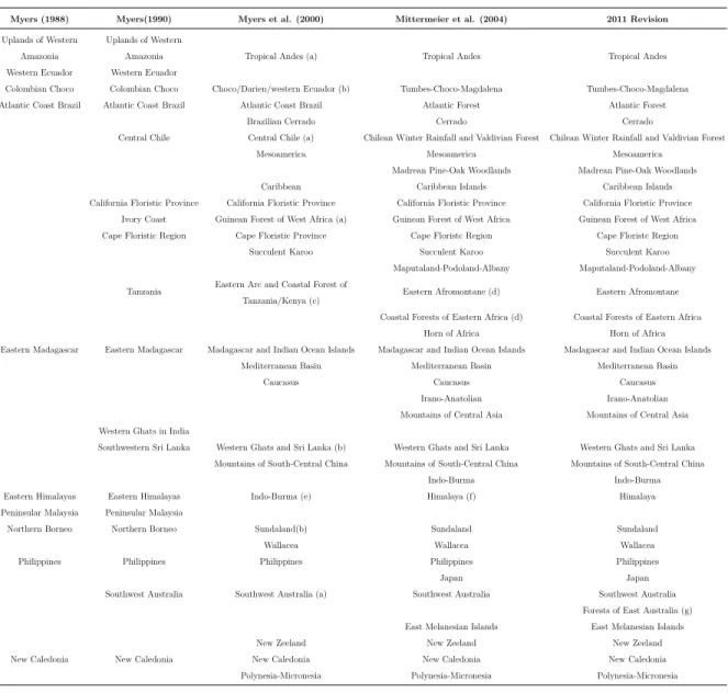
1 Biodiversity hotspots from 1988 to present (modified from Mittermeier et al. 2011) . . . 21
2 The proactive, reactive and representative approaches used for the se-lection of biodiversity conservation priority areas at global scale. All the approaches are based on a combination of the ecological criteria of vulnerability and irreplaceability (Modified fromSchmitt 2011) . . . 37
3 Gaussian-models for the different types of seasonal phytoplankton cycles 54
4 Main bloom phenology parameters extracted for each year at each pixel 54
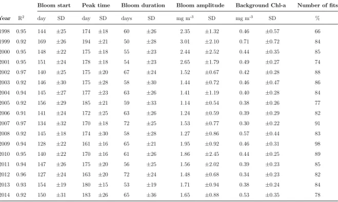
5 Summary of the annual average values (and standard deviation, SD) of the regional phenological parameters obtained from the Gaussian fits. R2
is the coefficient of determination of the Gaussian fits. The percentage of valid fits within the study region is also reported. . . 59
1 The figure shows the temperature anomaly trends from different inter-national science institutions. All show rapid warming in the past few decades and that the last decade has been the warmest on record (Source : https://climate.nasa.gov). . . 3
2 Arctic sea-ice volume is plotted for each day of the year, moving clockwise around the graph and taking one full year to complete a circuit. The volume of sea-ice on a particular day is represented by that plot’s distance from the center of the graph. Less sea-ice volume places the plot closer to the center (0%). Thin gray lines represent past years, while decadal averages and the current year (2018 in red) are thicker and color-coded as detailed in the legend . . . 4
3 The figure shows (a) the North Water (NOW) polynya located in northern Baffin Bay (>75°N) and southernmost (b) the Labrador Sea, a sub-polar sea that connects the North Atlantic with the Arctic Ocean. The Arctic Circle is also indicated (yellow line). The color gradient, from blue (low values) to red (high values), is given by the chlorophyll-a climatology derived from GlobColour (http://www.globcolour.info) images from 1998 to 2015. . . 12
4 The world’s biodiversity hotspots (see also Table 1 for hotspots names). Figure licensed under the Creative Commons Attribution-Share Alike 4.0 International license (Author: Conservation International). . . 23
5 North Water polynya is situated in northern Baffin Bay between Canada and Greenland. Smith Sound, the Arctic sea passage between Greenland and Ellesmere Island, links Baffin Bay with Kane Basin. Nares Strait (not indicated in the map) is the waterway between Ellesmere Island and Greenland that includes, from south to north, Smith Sound, and Kane Basin, respectively (a); monthly climatology of merged satellite chlorophyll-a data from April 1998 to September 2014 at 25 km of resolution within the NOW polynya: 74°N-81°N, 82°W-63°W (b); time series of 8-day composite images of chlorophyll-a, averaged for the NOW polynya from April 1998 to September 2014 (c) . . . 51
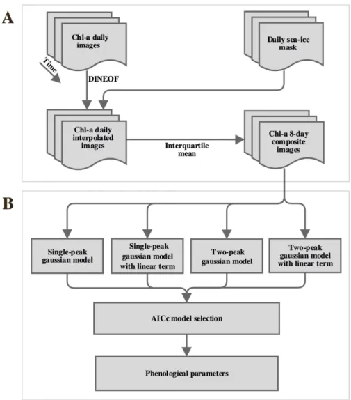
6 Workflow describing the multi-step tasks to obtain (a) 8-day compos-ite cloud-free chlorophyll-a images and (b) multiple-Gaussian models approach to increase the number of fits. . . 52
7 Climatology (1998-2014) maps of a) bloom start, b) bloom duration, c) bloom amplitude, d) sea surface temperature, e) wind stress, and f) sea-ice concentration . . . 61
8 Time series analysis of the main bloom phenology characteristics (bloom start, bloom duration, and bloom amplitude) and environmental param-eters (SST, wind stress, and SIC) averaged for the NOW polynya area. The black line is the mean ± standard deviation (shaded grey area). The red line represents linear trend (days year-1) for the 17-year time series. Coefficient of determination (r2) and probability levels (p) is shown for
each figure in the upper right box. . . 62
9 Spearman’s rank correlation (ρ) matrix (a) between phytoplankton pheno-logical parameters: BS (bloom start), BD (bloom duration), BA (bloom amplitude), and abiotic factors: SST (sea surface temperature), WS (wind stress), CF (cloud fraction), SIC ice concentration), SIE
(sea-ice extent), IRT ((sea-ice-retreat timing), OWP (open-water period), and D (frequency of wind-driven entrainment). The red color indicates a significant (p < 0.05) negative correlation, while the blue color indicates a significant (p < 0.05) positive correlation. The color gradient (from red to blue) indicates the magnitude of the correlation. The color white means that the correlation between indicators is not significant (p > 0.05) according to the Spearman correlation statistical test. Principal component analysis biplot (b) of: variables (red arrows; see text above for abbreviations) and years (1998-2014) represented by dots. . . 63
10 (a) Spatial distribution of the clusters obtained from the K-means analysis and (b) the mean biomass (chlorophyll-a) annual cycles in each cluster ±1 standard deviation (light grey area). The spatial distribution of each cluster constitutes a specific bioregion representative of a characteristic seasonal cycle. (c) Time (day of the year) of the maximum chlorophyll-a amplitude (i.e., the date at which the chlorophyll-a reaches its maximum value) for each bioregion. . . 90
11 Time series (2002-2014) of chlorophyll-a (green solid line), heat fluxes (the shaded areas show negative values in winter) and simulated mixed layer depth (green area) over the southern bioregion. The heat fluxes annual cycle is made up by negative values (cooling) in winter (grey shaded areas), which favors convective mixing and by positive values in spring-summer (period between grey shaded areas). The vertical (black dotted) lines represent the date (for each year) on which the heat fluxes became positive for a minimum of 20 consecutive days (note one time-step is 10-days). The mixed layer is still deep when chlorophyll-a starts growing at the end of winter and the heat fluxes change sign (black dotted lines). 93
12 (a) Net surface growth rate increase averaged over the southern bioregion (green solid line ±1 standard deviation) as a function of the days since the net heat fluxes turns positive. The average net surface growth rate is much larger closer to the date when the heat fluxes turns positive (i.e., day zero). (b) The mixed layer depth (from 2002 to 2014) at the time when the air-sea heat flux turned positive over the southern bioregion. Green bars represent the modeled mixed layer depth, while the black two-dashed line with successive segments represents the ARGO mixed layer depth (note that for the year 2002 no ARGO data were available at the time when the air-sea heat flux turned positive). In both cases, when heat fluxes first exceed zero the depth of the mixed layer is often deeper than 100 m. (c) The stratification index for both bioregions (see different colors) at the time when the HFs change sign over the southern bioregion (green bars). In 8 out of 13 years (∼62%) the stratification is stronger (i.e., larger N2) in the northern bioregion (yellow bars). . . 94
13 Time series (2002-2014) of chlorophyll-a (yellow solid line), stratification (grey areas), and simulated mixed layer depth (yellow area) over the northern bioregion. As the MLD shoals the stratification within the upper 25 m of the ocean increases. The vertical (black dotted) lines represent the date (for each year) of maximum mixed layer shoaling (i.e., the steepest gradient that occurs between its maximum and minimum). The vertical (red dashed) lines represent the date (for each year) on which the heat fluxes became positive. The cooling-to-heating shift in air-sea heat flux (red dashed lines) occurs, on average 1.9 ± 1.4 time-steps (with a range spanning from a minimum of 0 to a maximum of 5; note that one time-step is 10-days) after the shoaling of the MLD (black dotted lines). 99
14 Phytoplankton growth rates values at the time of the cooling-to-heating shift in air-sea heat flux over the northern bioregion. The red dashed line represents the average value, while the light grey area is ±1 standard deviation from the mean. Growth rates are near-zero or already negative (i.e., declining biomass). (b) Net surface growth rate increase averaged over the northern bioregion (yellow solid line ±1 standard deviation) as a function of the days since the mixed layer depth reaches the steepest gradient (i.e., becoming shallower) that occurs between its maximum and minimum. The average net surface growth rate is larger closer to the date on which the mixed layer depth became shallower (i.e., day zero). (b) The stratification index for both bioregions (see different colors) at
the time when the mixed layer depth reaches the steepest gradient in the northern bioregion. In 9 out of 13 years, the upper ocean stratification is much stronger over the northern bioregion. . . 100
15 Temporal and spatial characterization of remotely sensed surface, chlorophyll-a concentrchlorophyll-ation over the Lchlorophyll-abrchlorophyll-ador Sechlorophyll-a. (chlorophyll-a) Time-series (1998-2015) ob-tained from the mean of all chlorophyll-a values (in mg m-3) available
from eight-day composites of the Labrador Sea area between March 1998 and September 2015. Chlorophyll-a values (red dots) that were obtained from less than 30% of all pixels contained in the Labrador Sea area are also indicated. Maps showing (b) climatological (1998-2015) monthly mean of chlorophyll-a concentration for May; (c) monthly anomaly of chlorophyll-a for May 2011; and (d) monthly anomaly of chlorophyll-a for May 2015. In (d) the area of deepest mixing is indicated by the dashed black line. . . 114
16 (a) Time-series of the winter (December to March average) of the NAO index. (b) Correlation between the NAO and the convection depths. (c) Correlation between the depths of the winter convection and the surface chlorophyll-a (area-averaged from May to June) over the period 1998-2015. (d) Correlation between the Sub-Polar Gyre Index (SPG-I) and the area-averaged surface chlorophyll-a between 1998 and 2015. . . 117
17 Temporal and spatial characterization of altimetry-derived surface EKE (Eddy Kinetic Energy) and absolute geostrophic velocities over the Labrador Sea. (a) Time-series of altimetry-derived EKE in the Labrador Sea averaged between April and May (spring), for the period 1998-2015. Maps showing (b) the climatological (1998-2015) mean distribution of surface EKE in the Labrador Sea; (c) monthly anomaly of EKE in spring 2011; (d) monthly anomaly of EKE in spring 2015; (e) absolute geostrophic velocities average (May 1st; 1993-2015); (f) absolute geostrophic velocities
18 Eddy Kinetic Energy (EKE) seasonal cycle in the Labrador Sea for the years 2015 (green), 2011 (red) and the mean period (blue). The dark gray area indicates the period of deepest convection (February-April). The pale gray area indicates the bloom period (from late April to the end of May) over the year 2015. The 2015 spring bloom seems to coincide with a phase of increased eddy activity. . . 121
19 High-resolution images of chlorophyll-a (Chl-a) and Sea Surface Temper-ature (SST) the 17th of May 2015. On both sides, small boxes (from a
to f) of Chl-a and SST show more in details some of the small cyclonic eddies within the bloom area. . . 123
20 An example of fit. CHLB (0.38 mg/m3) corresponds to the background
chlorophyll-a determined by the fitted function (red line). CHL1 (1.91
mg/m3) correspond to the peak amplitude, ω
1 is the standard deviation
of the Gaussian curve and define the temporal width of the bloom, and tp1 (day 90 of year) define the peak timing, i.e. the day of the year at
which the maximum of bloom occurs. The bloom start is determined using a relative threshold : it is the date (day of the year) at which the fitted function reaches the threshold of 20% (blue line) of its maximum amplitude. The same criterion was used to define the bloom end in the downslope of the Gaussian curve. The time interval, represented in figure by the blue lines, gives the bloom duration (the difference between bloom end and bloom start). . . 134
21 Bloom start phenology : inter-annual differences for selected years (1998-2000, 2002, 2003, 2005, 2007, 2009, 2012, 2014) over the study region. White areas represent pixels with low variability or persistent periods of missing data. Highest values are represented by the red color and lowest values by the blue color. . . 135
22 Bloom duration phenology : inter-annual differences for selected years (1998-2000, 2002, 2003, 2005, 2007, 2009, 2012, 2014) over the study region. White areas represent pixels with low variability or persistent periods of missing data. Highest values are represented by the red color and lowest values by the blue color. . . 136
23 Bloom amplitude phenology : inter-annual differences for selected years (1998-2000, 2002, 2003, 2005, 2007, 2009, 2012, 2014) over the study region. White areas represent pixels with low variability or persistent periods of missing data. Highest values are represented by the red color and lowest values by the blue color . . . .137
24 Plot of the proportion of variances (y-axis) explained by the components (x-axis) of annual change in phytoplankton phenology and physical
pa-rameters across the years (1998-2014). Based on this figure, we decided to retain 4 principal components and to focus only on the two most important that represent more than 70% of the proportion of variances (Axe 1 = 57.4% ; Axe 2 = 15.7%) . . . 138
25 The Calinski-Harabazs index used to estimate the optimal number of cluster to bio-regionalize the Labrador Sea. The index measures the ratio between the dispersion of the observations (i.e., chlorophyll-a data) within a cluster and the dispersion between the clusters. The optimal clustering is the one with the highest value for the pseudo F-statistic. . . 140
26 Hovmöller diagram used to plot the latitudinal evolution of the 10-days climatological (2002-2014) chlorophyll-a mean as function of the time over the Labrador Sea. Compared to the North Atlantic where blooms tend to follow the general south-to-north progression, the reversed pattern within the Labrador Sea represents a distinctive feature. . . 141
27 Salinity values are from the surface layer (0-50 m) and were extracted from the World Ocean Database 2009 (https://www.nodc.noaa.gov). In the top panel, dots indicate individual original measurements (n = 45768). . . 142
28 Scatter plot comparing the time-series of mean MLD computed with the ANHA4 configuration and ARGO-floats using the density criteria. The mean from ARGO-floats was computed when there were more than five floats available after outliers were removed. Outliers were defined as values being more than two standard deviations from the mean. The model represents relatively well the shallower MLD (<200 m) with biases of only 8 meters (small panel on the right). . . 143
29 Standardized monthly anomalies maps of surface chlorophyll-a for the month of May over the period 1998-2015. Satellite data indicates elevated phytoplankton biomass in the Labrador Sea during May 2015 when compared to data for the eighteen-year period (1998-2015). . . 145
30 Depth-averaged (0-25 m) chlorophyll-a concentration in the central La-brador Sea derived from Biogeochemical-Argo (BGC-Argo) float mea-surements in May 2013 and 2015. The box in the upper left shows the free-drifting profiling floats position taken into account. . . 146
BS Bloom Start BD Bloom Duration BA Bloom Amplitude CF Cloud Fraction CHL-A Clorophyll-a
D Frequency of wind-driven entrainment EKE Eddy Kinetic Energy
HFs Heat Fluxes
IRT Ice-Retreat Timing MLD Mixed-Layer Depth
NAO North Atlantic Oscillation Index OWP Open-Water Period
SIC Sea-Ice Concentration SIE Sea-Ice Extent
SPG-I Sup-Polar Gyre Index WS Wind Stress
Marine phytoplankton blooms and their importance
Phytoplankton are mostly microscopic photosynthetic (single-celled and colonies) organisms that float freely in the uppermost sunlit layer of marine and freshwater ecosystems. Similar to terrestrial plants, phytoplankton contain chlorophyll to capture sunlight and use photosynthesis to turn it into chemical energy. Marine phytoplankton fuel the oceanic food web and through the photosynthetic carbon fixation (i.e., primary production) mitigate the oceanic and atmospheric carbon dioxide (CO2) levels (Sanders
et al., 2014). The Earth’s cycle of carbon and, to a large extent, its climate depend on these photosynthetic organisms that strongly influence ocean-atmosphere gas exchanges (Sanders et al.,2014).
Phytoplankton blooms (i.e., a condition of elevated phytoplankton concentration) are ubiquitous and recurrent phenomena that contribute significantly to annual primary production and to biogeochemical processes, such as the biological carbon pump, which transfer the organic carbon from the sunlit surface waters to the ocean interior (Diehl et al., 2015; Sanders et al., 2014;Tremblay et al., 2015). Phytoplankton blooms vary in timing, magnitude, and duration both spatially and inter-annually as a consequence of annual fluctuations in light and nutrient regime, water column stability (i.e., stratifica-tion) and grazing activity (Winder and Sommer,2012; Waniek, 2003). In particular, a phytoplankton bloom occurs when seasonal light limitation lapses due to the shoaling of the mixed layer above a critical-depth, where the loss terms (i.e., respiration, grazing, sinking and natural mortality) are largely compensated by photosynthetic production (the so-called "critical depth hypothesis" ; Sverdrup 1953).
However, although the "critical-depth hypothesis" formulated by Sverdrup (1953) remains the most cited and widely accepted theory, new physical and biological
me-chanisms have been suggested to drive phytoplankton blooms, especially in subarctic Atlantic. In recent years, different studies have agreed (Mahadevan et al.,2012), challen-ged (Behrenfeld,2010; Boss and Behrenfeld,2010) or merely refined Sverdrup’s model by testing the hypothesis that the shutdown of winter convective mixing could serve as a better indicator for the onset of the spring bloom than the mixed-layer depth (Taylor and Ferrari,2011). Recently observations (Lacour et al.,2017) showed evidence for widespread winter (January-March) phytoplankton blooms in a large part of the North Atlantic sub-polar gyre triggered by a combination of eddy-driven restratification and prolonged periods of calm (i.e., relaxation of atmospheric forcing). All these works highlight the complex interplay between abiotic and biotic factors in triggering the phyto-plankton bloom dynamics. Probably, there is not a single dominant physical mechanism that best predicts the inter-annual variability of the bloom onset (Ferreira et al., 2015). In this connection, to move beyond the “single mechanism” point of view, an integrated conceptual model of the physical and biological controls initiating the onset of the phytoplankton spring bloom has been proposed (Lindemann and St John,2014). Finally, it is becoming increasingly clear that the cells’ ability (i.e., adaptive qualities) to modify physiological rates in response to changes in the external environment may also play an important role in the onset of phytoplankton spring bloom (Lindemann et al.,2015). For instance, restratification during the winter period may cause a phytoplankton community shift from small phytoplankton cells (i.e., pico- and nano-) to micro-phytoplankton cells such as diatoms (Lacour et al., 2017). Overall, factors controlling the phytoplankton seasonal cycle dynamics still remain controversial.
High-latitude sea-ice cover and primary production in a changing climate : a briew overview
There is no doubt that global climate is changing. A considerable number of studies published in peer-reviewed scientific journals shows that ∼ 97% of actively publishing
climate scientists agree that climate-warming trends (Figure 1) over the past century are most likely due to human activities (Cook et al., 2016, 2013).
Figure 1: The figure shows the temperature anomaly trends from dif-ferent international science institutions. All show rapid warming in the past few decades and that the last decade has been the warmest on record (Source : https://climate.nasa.gov).
The impacts of climate warming are now increasingly visible in northern high-latitude ocean areas. In particular, the Arctic and subarctic marine ecosystems are experiencing a rapid sea-ice habitat loss and fragmentation that challenges the adaptive capacity of sea-ice dependent marine mammals (Moore and Huntington, 2008; Laidre et al., 2015) and under-ice fauna (Kohlbach et al., 2016). Changes in the sympagic biota (i.e., organisms that live in, on or associated with the ice, ranging from microbial communities to the charismatic mega-fauna, including seals, walrus and polar bears) are now more than evident.
The sea-ice extent, one of the largest biomes on Earth, has significantly decreased in recent decades (Comiso et al.,2008), hitting its lowest in 2012 (Parkinson and Comiso,
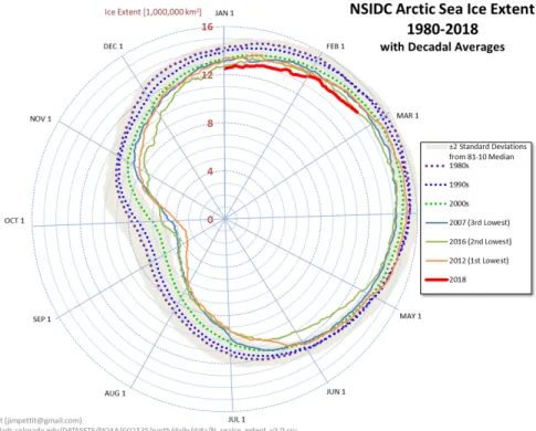
2013). More precisely, in September 2012 the average Arctic sea-ice extent (Figure 2) was the lowest in the satellite record. Other record lows occurred in September 2007 and recently in September 2016 (Figure 2). Based on estimates produced by the National Snow and Ice Data Center (NSIDC) Sea Ice Index (Fetterer et al., 2002) the September 2016 seaice minimum extent was 33% lower than the 1981-2010 average sea-ice minimum extent and tied with 2007 for the second lowest value in the satellite record (1979-2016). These recent observations strengthen even more the idea that the sea-ice cover is becoming more sensitive to ocean warming.
Figure 2: Arctic sea-ice volume is plotted for each day of the year, moving clockwise around the graph and taking one full year to complete a circuit. The volume of sea-ice on a particular day is represented by that plot’s distance from the center of the graph. Less sea-ice volume places the plot closer to the center (0%). Thin gray lines represent past years, while decadal averages and the current year (2018 in red) are thicker and color-coded as detailed in the legend
As temperatures have increased, much of the multiyear sea-ice has disappeared and been replaced by a markedly thinner first-year ice that melts earlier in spring (Maslanik et al., 2011; Ricker et al., 2017). As a result, the earlier melt has allowed an ever-increasing fraction of the sea surface to absorb more solar radiation, thus delaying the sea-ice freeze-up timing in the fall throughout most of the Arctic (Stroeve et al.,2014). A later freeze-up timing implies that the sea-ice has less time to thicken before the start of the next melt season, therefore resulting in its being more prone to melt. Basically, the heat gained by the ocean mixed-layer during summer feeds a loop that causes temperatures to rise : regions with especially higher than average temperatures correspond to regions with lower sea-ice extent (Stroeve et al., 2014). Moreover, intensification of the hydrological cycle is also predicted to occur due to increasing precipitation (Kopec et al., 2016), rivers discharge (Bring et al.,2017) and melting of glaciers and ice-sheets on land (Luo et al., 2016).
Although the ongoing changes in the physical domain are well documented, the response of the marine ecosystem to these major external disturbances is still uncertain. For instance, changes in sea-ice phenology (i.e., break-up, freeze-up and length of the open-water season) have regionally dependent and significant impacts on pelagic primary production (Wassmann and Reigstad,2011). Sea-ice plays an important role in promoting active biological and chemical processes and in regulating interactions between the upper ocean and the atmosphere (Budikova, 2009; Vancoppenolle et al., 2013). In particular, the sea-ice coverage directly influences the pelagic system by regulating the amount of solar radiation reaching the water column and thus limiting the length of the productive season (Arrigo and van Dijken,2011). Historically, regions underneath a full sea-ice cover (i.e., optically thick with a high reflection) have usually been considered incapable of supporting phytoplankton production. However, in the present-day Arctic the undergoing shift from multi-year ice to first-year ice caused the thinner summertime sea-ice to be increasingly covered by melt ponds, which efficiently transmit light to the underlying ocean (Frey et al.,2011;Palmer et al.,2014). Recent observations indicate that massive
phytoplankton blooms start beneath the sea-ice when under-ice light conditions are favorable (Arrigo et al., 2012). The presence of melt ponds may therefore stimulate the light-limited biological productivity. According to a recent study (Horvat et al.,
2017), at the present day nearly 30% of the ice-covered Arctic Ocean between June and July permits sub-ice blooms. However, even under favorable light conditions, nutrient availability can limit biological productions in sea-ice melt ponds (Arrigo et al.,2014;
Sørensen et al.,2017).
Connected with the sea-ice dynamics are sea-ice edge phytoplankton blooms, which occur when sea-ice retreats (Perrette et al.,2011). The sea-ice edge blooms can be favored by a shallow mixed-layer (i.e., due to warm and fresher water that minimizes vertical mixing), increasing light and by the release from melted ice of material (i.e., nutrients and metals) into the water column (Vancoppenolle et al.,2013). However, quantifying the contribution of primary production of the ice-associated blooms remains a challenge because of the lack of observational data (Perrette et al., 2011).
Both in situ and satellite observations are used to estimate the biological producti-vity (Matrai et al.,2013;Tremblay et al., 2015). In situ measurements directly estimate primary production throughout the water column (i.e., from surface to subsurface) but they are usually restricted to very small areas. Satellite ocean colour observations provide more extensive spatial and temporal coverage but are limited to the surface and affected by data gaps (Perrette et al.,2011). Overall, the increase in phytoplankton biomass and productivity over the Arctic Ocean has been based mainly on open-water measurements. For instance, satellite observations over a 12-year (1998-2009) period reported a 20% overall increase in primary production, mostly due to an increase in open-water extent (+27%) and duration (+45 days) of the open-water season (Arrigo and van Dijken,2011). A new study (Arrigo and van Dijken,2015) incorporating a more recent reprocessing version of the ocean color data suggests that primary production in the Arctic Ocean continues to increase rapidly. Other remote sensing studies (Petrenko
et al., 2013) and model simulation (Slagstad et al.,2015) suggest an increase, although unevenly, in primary production. However, although these estimates currently lack the ice-associated production, the observed enhancement in primary production has to be carefully considered. In high-latitude ocean areas, numerical models still lack validation with in situ time series (Babin et al., 2015). Furthermore, satellite-derived ocean-color models are still subject to large uncertainties (Lee et al., 2015) due to different metho-dological approaches and/or high concentrations of colored dissolved organic matter that impede clear-cut estimates of chlorophyll-a (Matsuoka et al., 2011; Matrai et al.,
2013) a key diagnostic marker of phytoplankton (Huot et al.,2007). Another source of uncertainty is the presence of a subsurface chlorophyll-a maximum (Ardyna et al.,2013), which can become more important on a regional scale and critical for the pelagic-benthic coupling system and higher-trophic-levels organisms (Wassmann and Reigstad, 2011). Finally, the role of increasing cloudiness on the light intensity reaching the water column and its effect on primary production has recently been debated (Bélanger et al.,2013a). The latter analysis suggests that although the duration of the open-water period may further increase, the phytoplankton photosynthetic activity might not follow a similar positive trend because it is light-limited (Bélanger et al., 2013a).
Against this background, it follows that one of the key issues is whether or not the ongoing changes will translate into enhanced phytoplankton production. Results suggest that the decrease in sea-ice cover should cause an increase in primary production by lengthening the growth season and allowing more sunlight to enter the sea-surface layer. However, as previously discussed, cloudiness may influence the length of the productive season by controlling the photosynthetic light requirement (Bélanger et al., 2013a). Moreover, the nutrient availability and distribution over the entire productive period is also of fundamental importance. Both factors (i.e., light and nutrient availability) have been found to limit primary production in the Arctic and subarctic seas (Tremblay et al.,2015). A recent study based on in situ measurements showed that the freshwater variability in the Chukchi Sea has a strong influence on primary production by lowering
the nutrient inventory in the euphotic zone (Yun et al.,2016). These results are consistent with those of previous studies (e.g.,McLaughlin and Carmack, 2010) that indicate that an increase in stratification may strongly limit the availability of nutrients and therefore negatively impact productivity. Some authors (e.g., Coupel et al., 2015) argued that despite higher light penetration, a further increase in freshening might lead the Arctic deep basins to become more oligotrophic because of a weaker nutrient entrainment into the seasonal mixed layer. Basically, the freshwater accumulation could lead to a decline in biological production because it restricts mixing of deep nutrients to the ocean surface. The greatest decrease in primary production is expected in those marine regions characterized by stratification-induced nutrient limitation (Slagstad et al.,2015). Due to the heterogeneity of Arctic and subarctic marine regions, the idea that strongly emerges is that photosynthetic production is expected to vary regionally (or even locally) on the basis of different environmental factors controlling phytoplankton blooms (Wassmann and Reigstad, 2011). For instance, a recent study suggests that the increase in phytoplankton biomass and productivity in southwest Greenland waters is likely triggered by a greater nutrient supply associated with glacial meltwater (Arrigo et al.,
2017). The nutrients released can be transported long distances and potentially fertilize surrounding areas (Arrigo et al., 2017). Besides, the nutrient load supplied by rivers seems to have a greater contribution at local scale but so far it does not appear to fuel a major portion of the overall pan-Arctic primary production (Tremblay et al.,2015). Certainly, these processes could become much more important in years to come.
Phytoplankton phenology in the Northern Hemiphere : a bottom-up synthe-sis
Most of the above-mentioned studies focus mainly on estimates of primary pro-duction. However, obtaining annual (seasonal) estimates of pelagic primary production should not obscure the importance of closely monitoring the phytoplankton seasonal
cycle dynamics (i.e., phenology : changes in timing, amplitude and duration). In marine ecology, phenological studies are increasingly used to inspect pelagic ecosystems’ response to changing climatic conditions. Phytoplankton phenology is a sensitive indicator useful in assessing the response of the pelagic ecosystems (Platt and Sathyendranath, 2008) to major external disturbances such as changes in water temperature and ice coverage. In particular, in northern high-latitude pelagic ecosystems, phytoplankton phenology requires special consideration for several reasons :
1. The strong seasonality in environmental conditions such as light, temperature, nutrients, snow and sea-ice cover heavily characterize this remote environment ; 2. The organism’s reproductive strategies are adapted to both the harsh conditions
and the narrow time window defined by the strong seasonality. For instance, phytoplankton blooms seasonality is strongly coupled with the light regime, which is influenced by the seasonal and latitudinal controls and by the presence of snow and sea-ice cover. The latter both attenuates and reflects light and is thus an important contributor to the phytoplankton growth cycle (Ji et al., 2010) ;
3. Even a small timing mismatch (Søreide et al., 2010) between the organism’s life strategy and the physical environment could have a substantial consequence for the entire food web. In particular, changes in bloom timing may affect the energy flow throughout the whole food web, which in turn may impact higher trophic level productivity (Malick et al., 2015) ;
4. Climate warming through mechanisms that influence water column conditions is predicted to lead marked and unexpected changes in Arctic and subarctic marine ecosystems (Wassmann et al.,2011). Continued climate warming can modify not only the bloom timing but also species composition and size structure, favouring species traits best adapted to changing conditions (Winder and Sommer, 2012).
Recent studies revealed that dramatic changes in bloom characteristics and pheno-logy have occurred in the Arctic and subarctic marine regions. According to Li et al.
(2009), the phytoplankton community composition has changed under the warming, freshening and stratifying condition in the Canada Basin. The authors revealed a shift toward a dominance of small phytoplankton cells. These findings are consistent with recent field observations (Blais et al., 2017) showing a drastic modification of the phyto-plankton community structure (from large to small cells) and a drop in phytophyto-plankton biomass between 1999 and 2011 in the north of Baffin Bay. Changes in phytoplankton community composition have also been reported in the Chukchi Sea and correlated with the sea-ice retreat timing (Fujiwara et al., 2014). Using satellite data, Kahru et al. (2011) reported significant trends (from 1997 to 2009) towards earlier (up 3-5 days per year) phytoplankton blooms in Arctic Ocean and peripheral seas. Particular regions experiencing earlier blooms include e.g., the Hudson Bay, Baffin Sea, off the coasts of Greenland and Kara Sea, which are also areas roughly coincident with trends toward earlier summer ice break-up (Kahru et al., 2011). Model outputs together with satellite data also suggest that changes in ice-retreat timing have a strong impact on the timing variability in pelagic phytoplankton and ice-algae peaks (Ji et al., 2013). As an example, in the Barents Sea, phytoplankton blooms are triggered by different stratification mechanisms : heating of the surface layers in ice-free waters and melting of the sea-ice along the ice edge (Oziel et al., 2017). Another study (Zhai et al., 2012) also detected earlier blooms north of the Iceland-Faroe area (Arctic waters) due to early stratification and a later bloom in the southern area (Atlantic waters) characterized by a weakly stratified water-column. In Greenland, Iceland and Norwegian seas, results from a biophysical model showed that earlier phytoplankton blooms lead to an earlier and more severe nutrient drawdown (Zhang et al., 2010). Further south, in the Baltic Sea, satellite observation (from 2000 to 2014) indicates that while bloom timing and duration co-vary with meteorological conditions, the bloom magnitude is mainly determined by winter nutrient concentration (Groetsch et al., 2016). In the Labrador Sea, the positive relationship between deep winter (convective) mixing and nutrients concentration creates favorable conditions for phytoplankton growth in spring and summer (Harrison et al.,
2013). Recent increases in Arctic freshwater flux may weak convective mixing (Yang et al., 2016) and thereby potentially lead to a significant reduction in phytoplankton production. Howwever, a progressive deepening of winter convection in the Labrador Sea was observed since 2012 (Yashayaev and Loder, 2017).
On the above basis, it seems clear that in northern high-latitude oceans the seasonality of the phytoplankton bloom is controlled primarily by sea-ice dynamics, light and nutrient availability. In this context, the interplay between stratification and mixing plays a fundamental role in shaping the biological production. Stratification causes the retention of phytoplankton within the euphotic layer, making light more available but limiting access to inorganic nutrients. Light levels and the availability of nutrients can therefore vary according to the intensity of the vertical stratification. The latter in turn depends upon the temperature and salinity gradients as well as vertical mixing processes (Drinkwater et al., 2010). It follows that changes in physical forcing result in a modification of the balance between stratification and mixing. For instance, although freshwater strengthens the stratification, a reduced sea-ice cover exposes an ever-increasing fraction of the water column to wind-induced mixing processes. Periodic vertical mixing, driven by wind events enhancing the nutrient replenishment, can therefore burst and sustain the biological production, eventually throughout the growing season (Tremblay et al., 2011, 2015). Recently, Ardyna et al.(2014) using satellite data, documented a fundamental shift from a polar to a temperate mode. The development of a second bloom in several regions of the Arctic and sub-arctic oceans seems to coincide with the delayed freeze-up and the increased exposure of sea surface to wind stress.
Figure 3: The figure shows (a) the North Water (NOW) polynya located in northern Baffin Bay (>75°N) and sou-thernmost (b) the Labrador Sea, a sub-polar sea that connects the North Atlantic with the Arctic Ocean. The Arctic Circle is also indicated (yellow line). The color gra-dient, from blue (low values) to red (high values), is given by the chlorophyll-a climatology derived from GlobColour (http://www.globcolour.info) images from 1998 to 2015.
Thesis objectives and study areas
The large seasonality in light, temperature, and sea-ice extent is an integral aspect of the Arctic and subarctic marine regions. However, the continuous Arctic-wide decrease in sea-ice cover and its amplifying effect on the warming are modifying abiotic (e.g., balance between stratification and mixing) and biotic (e.g., grazing) mechanisms (Winder and Sommer, 2012). In present-day climate conditions, monitoring the extent of the shifts in timing together with the spatial distribution of phytoplankton blooms is relevant because of their influence on biogeochemical cycles and marine ecosystem structure and functioning. A better understanding of the phytoplankton response to these ongoing environmental alterations may therefore provide a sensitive indicator of climate change.
Therefore, given the central role of phytoplankton in marine ecosystems, the main objectives of this thesis are (1) to detect and quantify changes in timing, magnitude, duration and spatial distribution of phytoplankton blooms in Arctic and subarctic regions recognized as marine biological hotspots ; and (2) to relate these changes with variability in oceanic and meteorological forcing mechanisms.
To accomplish these goals we used a remote sensing approach supplemented by in situ measurements and models outputs. While essential knowledge on marine ecosystem structure and functioning will continue to be derived from specific in situ observations, the estimation of biological parameters (such as chlorophyll-a) through satellite remote sensing provides a powerful tool to characterize phytoplankton phenology at local, regional and global scales. Although satellite observations are limited to the ocean surface, the possibility of periodically mapping areas at relatively high temporal frequency provide compensating benefits.
The study was conducted at regional (and sub-regional scale) in two marine areas (Figure 3) sensitive to the effects of ongoing climate changes and considered as hotspots
1. The North Water (NOW) polynya, located between Greenland and Ellesmere Island in northern Baffin Bay is the largest and one of the most biologically productive marine areas of the Arctic Ocean. The NOW serves as an important winter and summer habitat for marine birds and mammals and is considered an oceanographic “window” through which it is possible to evaluate the state of the Arctic marine ecosystem ;
2. The Labrador Sea, a sub-polar sea that connects the North Atlantic with the Arctic Ocean, represents a major focal point for ocean feedback to the climate system. It is a region characterized by a pronounced seasonality in biological production. The northern part of Labrador Sea host one of the largest phytoplankton spring bloom of the whole North Atlantic Ocean, with surface area that can reach as much as 700 000 km2. In addition, deep convection and biology processes work together
making the Labrador Sea one of the principle oceanic “sinks” for atmospheric carbon dioxide of the World Ocean.
This thesis includes a review (Chapter 1) of the current literature on the general concept of hotspots, three research articles (Chapters 2-4) and a general conclusion. Specifically, the chapters of this thesis addressed the following topics :
Chapter 1 provides a comprehensive review to introduce the approach that lies behind the concept of biodiversity hotspots. The main criticisms and controversies concerning this approach are also discussed. Next, links between biodiversity hotspots, marine pelagic ecosystem processes and the deep-sea realm are taken into consideration. Finally, some challenges in assigning global conservation priorities are briefly discussed. This chapter was done as part of the Ph.D. program and specifically in relation to the course Synthèse Environnementale. This chapter was published in Global Ecology and Conservation (Marchese, 2015).
Chapter 2 begins the research part of this thesis. The specific objective of this study is to investigate how contrasting effects of environmental factors may modulate
the phytoplankton bloom response over the North Water (NOW) polynya. A novel framework that combines an improved interpolation scheme to fill data gaps together with Gaussian-models is used to increase accuracy when phenology metrics were applied. This chapter was published in Polar Biology (Marchese et al., 2017). Chapter 3 focuses on the bloom onset variability over the whole Labrador Sea. A
biogeographic analysis is used to partition the Labrador Sea into regions with similar phytoplankton variability. Finally, the relationships between the spring bloom onset and physical forcing are investigated using satellite-derived ocean color observations and simulated data from a state-of-the-art ocean global circulation model (CGM). This chapter is at an advanced preparation stage and will be submitted to an high-impact and high-quality peer-reviewed journal at the earliest possible date.
Chapter 4 provides evidence for the occurrence of an anomalous springtime phyto-plankton bloom that occurred in the Labrador Sea in 2015. The study, by using a combination of satellite and in situ observations, attempts to elucidate the me-chanisms behind the extensive 2015 spring bloom. This chapter requires a little bit more work before being sent as a research letter to a scientific peer-reviewed journal.
The general conclusion reviews the main findings, highlights some possible limita-tions of the present study and presents a brief discussion on future research direclimita-tions.
BIODIVERSITY HOTSPOTS: A SHORTCUT FOR A MORE COMPLICATED CONCEPT
Global Ecology and Conservation 2015, 3, 297-309 Christian Marchese1
1Université du Québec à Rimouski, Département de biologie, chimie et géographie, 300
1.1 Résumé
Dans une ère caractérisée par l’activité humaine, les changements de l’environnement planétaire, la perte d’habitat et la disparition des espèces, les stratégies de conserva-tion marquent une avancée décisive pour réduire la perte de biodiversité. C’est le cas notamment de l’acidification des océans et du changement d’affectation des terres qui s’intensifient en plusieurs endroits, et dont les conséquences sont souvent irréversibles pour la biodiversité. Bien que critiqués, les points névralgiques de la biodiversité sont devenus des éléments clés pour élaborer les priorités de conservation et jouent un rôle important dans les décisions et stratégies économiques en matière de préservation de la biodiversité des écosystèmes terrestres, et marins, par extension. Cette action locale, applicable à toute échelle géographique, est tenue pour l’une des meilleures approches pour maintenir une large part de la diversité biologique mondiale. En revanche, la délimitation des points névralgiques repose à la fois sur des critères quantitatifs et des considérations subjectives, d’où le risque de négliger certaines zones, comme les points froids, dont la valeur de conservation pourrait sembler moindre. Or il est largement reconnu de nos jours que la biodiversité va bien au-delà du nombre d’espèces dans une région donnée et qu’une stratégie de conservation ne saurait simplement se baser sur le nombre de taxa dans un écosystème. L’idée qui s’impose de plus en plus, par conséquent, est la nécessité de revoir les priorités de conservation sur la base d’une approche interdisciplinaire qui en passe par la mise en place de partenariats politiques et scientifiques.
Mots clés : changement climatique, points froids, richesse spécifique, diversité phylogénétique, services écosystémiques
1.2 Abstract
In an era of human activities, global environmental changes, habitat loss and species extinction, conservation strategies are a crucial step toward minimizing biodiversity loss. For instance, oceans acidification and land use are intensifying in many places with negative and often irreversible consequences for biodiversity. Biodiversity hotspots, despite some criticism, have become a tool for setting conservation priorities and play an important role in decision-making for cost-effective strategies to preserve biodiversity in terrestrial and, to some extent, marine ecosystems. This area-based approach can be applied to any geographical scale and it is considered to be one of the best approaches for maintaining a large proportion of the world’s biological diversity. However, delineating hotspots includes quantitative criteria along with subjective considerations and the risk is to neglect areas, such as coldspots, with other types of conservation value. Nowadays, it is widely acknowledged that biodiversity is much more than just the number of species in a region and a conservation strategy cannot be based merely on the number of taxa present in an ecosystem. Therefore, the idea that strongly emerges is the need to reconsider conservation priorities and to go toward an interdisciplinary approach through the creation of science-policy partnerships.
Keywords: climate change, Coldspots, Species richness, Phylogenetic diversity, Ecosystem services
1.3 Introduction
As demonstrated by several researches, maintaining biodiversity is essential to the supply of ecosystem services and not less important to support their health and resilience (Pereira et al., 2013). However, despite there being an international interest to sustain and protect biodiversity, its loss does not seem to slow down (Butchart et al.,
2010). Although there has been an extension of protected areas (Pimm et al., 2014), these provide a still low species coverage (Venter et al., 2014) and do not appear to optimally protect biodiversity (Pimm et al., 2014). For instance, a recent analysis for conservation priorities in marine environments by combining spatial distribution data for nearly 12,500 species with human impacts information, identified new areas of high conservation value that are located in Arctic and Antarctic Oceans and beyond national jurisdictions (Selig et al., 2014).
Overall, habitat change and their over-exploitation, pollution, invasive species and in particular climate change are the major causes for biodiversity loss. The combined effect of these anthropogenic pressures may have already started a critical transition toward a tipping point (Barnosky et al., 2012). In particular, climate is modifying rapidly forcing biodiversity to adapt either through the change of habitat and life cycles or the development of new physical traits (Berteaux et al., 2010). For instance, rising temperatures can lead to potential biodiversity increases in northern regions (i.e., northern biodiversity paradox) where low temperatures usually are a limiting factor for the establishment of many species (Berteaux et al., 2010). Given the importance that biodiversity plays, the understanding of the main threats to biodiversity is today than ever before a central objective in conservation biology. Nowadays there is serious concern about the effectiveness of existing strategies for biodiversity protection. A central issue in conservation is to identify biodiversity-rich areas to which conservation resources should be directed. Based on the observation that some parts of the world have far more species than others, the area-based approaches are widely advocated for species
conservation planning. Areas with high concentrations of endemic species (species that are found nowhere else on Earth) and with high habitat loss are often referred to as ”hotspots” (Myers, 1988). The hotspot approach can be applied at any geographical scale and both in terrestrial and marine environments. However, hotspots represent conservation priorities in terrestrial ecosystems but remain largely unexplored in marine habitats (Worm et al., 2003) where the amount of data is still poor (Mittermeier et al.,
2011).
Despite this lack of homogeneity in data between terrestrial and aquatic ecosystems, the recent concerns over loss of biodiversity have led to calls for the preservation of hotspots as a priority. As reported by Myers(2003) at the end of his article, "Edward O. Wilson, one of the leading authorities on conservation, described the hotspot approach as "the most important contribution to conservation biology of the last century"". Closely linked to the concept of biodiversity, the hotspot concept is used with increasing frequency in biology and conservation literature and often with different meanings. While in a strict sense, the meaning is based on an estimate of endemic species and habitat loss, in a broad sense it refers to any area or region with exceptionally high biodiversity at the ecosystem, species and genetic levels.
The aim of this work is to review the current literature on the general concept of hotspots. We first introduce the approach that lies behind the concept of hotspots, in both terrestrial and marine ecosystems. Next we discuss the main criticisms and controversies concerning this approach and we present the possibility of using different alternative metrics to identify hotspots. Then we bring to light the links between biodiversity hotspots and marine pelagic ecosystem processes and we briefly introduce the deep-sea, a realm for the most part unknown for which several key questions are still waiting for an answer. Finally, we briefly discuss additional approaches and criteria, such as costs, in order to highlight some challenges in assigning global conservation priorities.
Table 1: Biodiversity hotspots from 1988 to present (modified fromMittermeier et al. 2011)
Myers (1988) Myers(1990) Myers et al. (2000) Mittermeier et al. (2004) 2011 Revision
Uplands of Western Uplands of Western
Amazonia Amazonia Tropical Andes (a) Tropical Andes Tropical Andes Western Ecuador Western Ecuador
Colombian Choco Colombian Choco Choco/Darien/western Ecuador (b) Tumbes-Choco-Magdalena Tumbes-Choco-Magdalena Atlantic Coast Brazil Atlantic Coast Brazil Atlantic Coast Brazil Atlantic Forest Atlantic Forest
Brazilian Cerrado Cerrado Cerrado
Central Chile Central Chile (a) Chilean Winter Rainfall and Valdivian Forest Chilean Winter Rainfall and Valdivian Forest Mesoamerica Mesoamerica Mesoamerica
Madrean Pine-Oak Woodlands Madrean Pine-Oak Woodlands Caribbean Caribbean Islands Caribbean Islands California Floristic Province California Floristic Province California Floristic Province California Floristic Province
Ivory Coast Guinean Forest of West Africa (a) Guinean Forest of West Africa Guinean Forest of West Africa Cape Floristic Region Cape Floristic Province Cape Floristc Region Cape Floristc Region
Succulent Karoo Succulent Karoo Succulent Karoo Maputaland-Podoland-Albany Maputaland-Podoland-Albany Tanzania Eastern Arc and Coastal Forest of
Tanzania/Kenya (c)
Eastern Afromontane (d) Eastern Afromontane
Coastal Forests of Eastern Africa (d) Coastal Forests of Eastern Africa Horn of Africa Horn of Africa Eastern Madagascar Eastern Madagascar Madagascar and Indian Ocean Islands Madagascar and Indian Ocean Islands Madagascar and Indian Ocean Islands
Mediterranean Basin Mediterranean Basin Mediterranean Basin
Caucasus Caucasus Caucasus
Irano-Anatolian Irano-Anatolian Mountains of Central Asia Mountains of Central Asia Western Ghats in India
Southwestern Sri Lanka Western Ghats and Sri Lanka (b) Western Ghats and Sri Lanka Western Ghats and Sri Lanka Mountains of South-Central China Mountains of South-Central China Mountains of South-Central China
Indo-Burma Indo-Burma Eastern Himalayas Eastern Himalayas Indo-Burma (e) Himalaya (f) Himalaya Peninsular Malaysia Peninsular Malaysia
Northern Borneo Northern Borneo Sundaland(b) Sundaland Sundaland
Wallacea Wallacea Wallacea
Philippines Philippines Philippines Philippines Philippines
Japan Japan
Southwest Australia Southwest Australia (a) Southwest Australia Southwest Australia Forests of East Australia (g) East Melanesian Islands East Melanesian Islands New Zeeland New Zeeland New Zeeland New Caledonia New Caledonia New Caledonia New Caledonia New Caledonia
Polynesia-Micronesia Polynesia-Micronesia Polynesia-Micronesia (a) Expanded.
(b) Merged and/or expanded.
(c) Expanded to include Coastal Forests of Tanzania and parts of Kenya.
(d) The Eastern Arc and Coastal Forests of Tanzania/Kenya hotspots was split into the Eastern Afromontane hotspot (the Eastern Arc Mountains and Southern Rift, the Albertine Rift, and the Ethiopian Highlands) and Coastal Forests of EasternAfrica (southern Somalia south through Kenya, Tanzania and Mozambique).
(e) Eastern Himalayas was divided into Mountains of South-Central China and Indo-Burma, the latter of which was expanded. (f) The Indo-Burma hotspot was redefined, and the Himalayan chain was separated as a new Himalayan hotspot, which was expanded. (g) The Forests of Eastern Australia the 35th biodiversity hotspot.
1.4 Biodiversity hotspots
1.4.1 The biodiversity hotspots concept
The British ecologist Norman Myers first published the biodiversity hotspot thesis in 1988. Myers, although without quantitative criteria but relying solely on the high levels of habitat loss and the presence of an extraordinary number of plant endemism, identified ten tropical forest "hotspots" (Mittermeier et al., 2011). A subsequent anal-ysis (Myers, 1990) added a further eight hotspots, including four in Mediterranean regions. Conservation International (CI: http://www.conservation.org) adopted My-ers’ hotspots as its institutional blueprint in 1989, and afterwards worked with him in a first systematic update of the global hotspots. Myers, Conservation International, and collaborators later revised estimates of remaining primary habitat and defined the hotspots formally as biogeographic regions with >1500 endemic vascular plant species and ≤30% of original primary habitat (Myers et al.,2000). This collaboration, which led to an extensive global review (Mittermeier et al., 1999) and a scientific publication (Myers et al., 2000) saw the hotspots expand in area as well as in number, on the basis of both the better-defined criteria and new data. A second major revision and update in 2004 (Mitttermeier et al.,2005) did not change the criteria but by redefining several hotspots boundaries, and by adding new ones that were suspected hotspots for which sufficient data either did not exist or were not easily accessible, brought the total to 34 biodiversity hotspots (Mittermeier et al., 2011). Recently, a 35th hotspot was added (Williams et al., 2011), the Forests of East Australia. The 35-biodiversity hotspots (Table 1; Figure 4) that cover only 17.3% of the Earth’s land surface are characterized by both exceptional biodiversity and considerable habitat loss (Myers et al., 2000). More precisely, hotspots maintain 77% of all endemic plant species, 43% of vertebrates (including 60% of threatened mammals and birds), and 80% of all threatened amphibians (Mittermeier et al., 2011; Williams et al., 2011).
Figure 4: The world’s biodiversity hotspots (see also Table 1 for hotspots names). Figure licensed under the Creative Commons Attribution-Share Alike 4.0 International license (Author: Conservation International).
Biodiversity is important in the oceans as on land. Myers and colleagues, however, excluded the oceans from their analysis. In particular, coral reefs are one of the most biologically diverse ecosystems in the ocean and provide important structures and habitat in tropical and sub-tropical coastal waters (Bellwood et al.,2004). In these areas, where the explanation for the high number of species is still debated (Bowen et al., 2013;
Cowman and Bellwood,2013), ocean acidification and changes in sea surface temperature (Ateweberhan et al., 2013) are likely to cause major coral reef losses and changes in the distribution and relative abundances of marine organisms. Moreover, apart from the intrinsic biodiversity value, there are economic arguments for the protection of marine biodiversity (Balmford et al., 2002). This makes the maintenance of marine biodiversity a valuable environmental management goal. Roberts et al. (2002), through the publication of one of the most comprehensive studies of hotspots on global coral reefs, have brought much-needed attention to marine hotspots, extending the hotspot concept to coral reefs and arguing that biodiversity hotspots are major centers of endemism in the sea as well as on land. Overall, the analysis revealed the 18 richest multi- taxon