Non Linear Proper Generalized Decomposition method applied to the magnetic simulation of a SMC microstructure

(1)

is an open access repository that collects the work of Arts et Métiers Institute of

Technology researchers and makes it freely available over the web where possible.

This is an author-deposited version published in: https://sam.ensam.eu Handle ID: .http://hdl.handle.net/10985/7815

To cite this version :

Thomas HENNERON, Abdelkader BENABOU, Stéphane CLENET - Non Linear Proper

Generalized Decomposition method applied to the magnetic simulation of a SMC microstructure -IEEE transactions on Magnetics - Vol. 48, n°11, p.3242 - 3245 - 2012

Any correspondence concerning this service should be sent to the repository Administrator : [email protected]

(2)

Non Linear Proper Generalized Decomposition method applied to the

magnetic simulation of a SMC microstructure

T. Henneron

1

, A. Benabou

1

, S. Clénet

2

1_{L2EP/Université Lille1, Cité Scientifique - 59655 Villeneuve d’Ascq, France} 2_{L2EP/Arts et Métiers ParisTech, 8 boulevard Louis XIV - 59046 Lille Cedex, France}

Improvement of the magnetic performances of Soft Magnetic Composites (SMC) materials requires to link the microstructures to the macroscopic magnetic behavior law. This can be achieved with the FE method using the geometry reconstruction from images of the microstructure. Nevertheless, it can lead to large computational times. In that context, the Proper Generalized Decomposition (PGD), that is an approximation method originally developed in mechanics, and based on a finite sum of separable functions, can be of interest in our case. In this work, we propose to apply the PGD method to the SMC microstructure magnetic simulation. A non-linear magnetostatic problem with the scalar potential formulation is then solved.

Index Terms— Soft Magnetic Composites, Non Linear Proper Generalized Decomposition

I. INTRODUCTION

oft Magnetic Composites (SMC) are magnetic materials offering an interesting alternative to the use of classical laminated iron steel in electromagnetic energy conversion [1]. Nevertheless, their magnetic and mechanical performances still remain below those of laminated magnetic steel. In order to improve the SMC performances, it is necessary to investigate their properties at the microstructure scale and to link them with the macroscopic behavior that is of interest for

the designer of electromagnetic devices. Previous

investigations have been realized [2] in order to reconstruct

the macroscopic magnetic behavior law from the

microstructure geometry. Interesting results have been obtained by the use of a classical 2D Finite Element (FE) calculation approach based on the geometry reconstruction using imaging obtained from the Scanning Electron Microscope (SEM). Nevertheless, the procedure is strongly linked to a rather delicate image processing step. In fact, the contours of the particles are interpolated between the pixels of the image. This step can introduce some error on the geometry model. It is then interesting to investigate other numerical techniques such as the Proper Generalized Decomposition (PGD) method [3,4,5]. This approach allows representing the solution separately on each geometric axis with functions approximated by a 1D FE discretization [3,5]. The main interest is that we have to solve several 1D FE systems instead of a 2D FE system, but it also avoids the geometry reconstruction as required in [2] for the 2D FE approach.

In this work, the PGD approach is applied to a simple, but representative, image of a SMC microstructure. The equivalent non-linear magnetic behavior of the studied microstructure is then calculated. In a first part, the problematic and the magnetostatic problem are briefly presented. In the second part, the non-linear PGD approach is developed. Finally, the results obtained from the PGD are

presented and compared with a reference 2D FE model.

II. POSITIONING OF THE PROBLEM A. Problematic

Whatever the chosen numerical approach, it is first necessary to perform the microstructure imaging in order to identify the distribution of the different materials. For the magnetic calculation, the porosities and the resin, that is used to agglomerate the iron particles, are considered with the air properties whereas the particles are considered with pure iron magnetic properties.

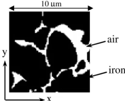
In the classical FE approach, it is necessary to extract the geometry in order to build a numerical model based on a mesh. This step is rather delicate as it requires an image processing procedure that must reflects with accuracy the real particle shapes and air gaps thicknesses. In fact, at the microstructure level, the material is strongly inhomogeneous and simulations have proven that the way the image processing is carried out has an impact on the magnetic behavior that is simulated. An alternative is to treat the image using each pixel as an element of the mesh (quadrangle elements in 2D). Nevertheless, in both cases, the bigger the image is, the higher the memory and computational cost will be. In this work, we focus on the accuracy of the method regarding the global behavior representation of a SMC microstructure simulation. Figure 1 shows the example of the microstructure that is actually studied.

x

y

air

iron

Fig. 1. Studied microstructure obtained from SEM

S

10 µm

Manuscript received January 1, 2008 (date on which paper was submitted for review). Corresponding author: T. Henneron (e-mail: [email protected]).

(3)

B. Mathematical model

Let us consider a domain D of boundary Γ (Γ=ΓB∪ΓH1∪ΓH2

and ΓB∩ΓH1∩ΓH2=0) (Fig. 2). We denote by ε the

magnetomotive force between ΓH1 and ΓH2 and Φ the magnetic

flux flowing through the domain.

ΓB ΓH1 D ΓB ΓH2 air iron iron iron ε Φ

Fig.2. Magnetostatic problem

The magnetostatic problem can be described by the following Maxwell’s equations,

curl H = 0 div B = 0 B = µ(H) H (1) (2) (3) with B the magnetic flux density, H the magnetic field, µ(H)

the non-linear magnetic permeability that depends on the magnetic field. The unicity of the solution is obtained by boundary conditions such that,

B.n=0 on ΓB and H×n=0 on ΓH1 and ΓH2 (4)

with n the outward unit normal vector. To solve the previous problem, the magnetic scalar formulation can be used by defining a magnetic scalar potential Ω in the whole domain. The magnetomotive force is introduced by a scalar function α [6] and the magnetic field can be expressed such that,

H = -grad Ω - ε grad α with Ω = cst on ΓH1 and ΓH2

and α = 1 on ΓH1 and α = 0 on Γ-ΓH1

(5)

Combining (3) and (5) in relation (2), we obtain the magnetic scalar potential formulation of the problem. The weak form to be solved is then written,

dD Ω' α. ε µ dD Ω' Ω. µ D (H) D (H)

∫

grad grad =− grad grad ₍₆₎

with Ω’ a test function defined in the same space as Ω. III. PROPER GENERALIZED DECOMPOSITION A. Separated representation

In order to solve (6), a method based on the PGD approach can be used [3, 4, 5]. Then, the scalar potential is approximated by a separated representation in the spatial dimensions x and y:

∑

= ⋅ ≈ Ω M 1 n n n(x) S (y) R y) (x, (7)

with x∈Dx, y∈Dy and M the number of modes. To

approximate Rn(x) and Sn(y), functional spaces of finite

dimension are introduced, i.e. 1D nodal shape function space. To compute the functions Rn(x) and Sn(y), an iterative

enrichment method is used. The couple (Rn(x), Sn(y)) is

calculated regarding the previous couples (Ri(x), Si(y)) with

i∈[1,n-1]. The function Ω’ (see (6)) can be written such that: (y)' S (x) R (y) S (x)' R y) (x, ' = _n ⋅ _n + _n ⋅ _n Ω (8)

with Rn(x)’ and Sn(y)’ the test functions defined in the same

spaces of Rn(x) and Sn(y) respectively.

The scalar function α used to impose the magnetomotive force is also expressed by a separated representation such that:

(y) (x).α α y)

α(x, = x y (9)

The 1D scalar functions αx(x) and αy(y) are discretized in the

same way as Rn(x) and Sn(y). The magnetic behavior law of

the microstructure is represented by a matrix Mµ which terms

correspond to the magnetic permeability associated to each pixel of the image (either iron or air). The magnetic behavior law is also expressed by a separated representation that uses functions defined on each axis. These ones are deduced from a Singular Value Decomposition (SVD) method [5], i.e. the magnetic permeability matrix is written such that,

∑

= = = N 1 j t j jj j t µ UDV UD V M (10)

with D the diagonal matrix of the singular values, U and V the matrixes of the left and right singular vectors, N the number of non zero singular values and “j” stands for the jth vector. The number of lines of U and V depend on the spatial discretization of the image, i.e. the number of pixels npx and

npy along x and y axes. From this decomposition, it is possible

to express the magnetic permeability µ(x,y) for a given position (x,y) in the domain such that,

∑

= = = = = = y x np 1 e' je' e' j np 1 e je e j N 1 j j j jj (y).V w (y) v and (x).U w (x) u with (y) (x)v u D y) µ(x, (11)

where wpx(x), resp. wpy(y), is the scalar interpolation function

associated to the pixel px, resp. py. This function is equal to 1

if x belongs to the pixel position and 0 otherwise. The permeability in (11) corresponds to a given magnetic state.

B. Determination of (Rn(x),Sn(y))

Each couple (Rn(x),Sn(y)) is calculated by solving iteratively

two equations determined from (6). First, we suppose that Sn(y) is known. Then, the function Sn(y)’ vanishes in (8) and

(4)

then solved in order to determine the function Rn(x) using the following expression,     − − −     − =     +    

∑ ∫

∫

∑ ∫

∫

∑

∫

∑

− = − = = = 1 n 1 D D x ' n i j y n i j 1 n 1 D D x ' i j y n i j D D x ' n x j y n y j N 1 j D D x ' x j y n y j jj D D x ' n n j y n n j D D x ' n j y n n j N 1 j jj y x y x n y x y x n y x y x n dD .R R u dD dy dS . dy dS v dD dx dR . dx dR u dD .S S v dD .R α u dD dy dS . dy dα v ε dD dx dR . dx dα u dD .S α v ε D dD .R R u dD dy dS . dy dS v dD dx dR . dx dR u dD .S S v D i i (12)

In a second step, we compute the function Sn(y) assuming that

the function Rn(x) is known. In this case, the function Rn(x)’

vanishes in (8) and the test function Ω’ is equal to Rn(x).Sn(y)’. To determine Sn(y), the relation (6) is solved

such that,     − − −     − =    

∑ ∫

∫

∑ ∫

∫

∑

∫

∑

− = − = = = 1 n 1 i D D y ' i j x n i j 1 n 1 i D D y ' i j x n i j D D y ' y j x n x j D D y ' y j x n x j N 1 j jj D D y ' n j x n n j D D y ' n j x n n j N 1 j jj x y n x y n x y n x y n x y n x y n dD .S S v dD dx dR . dx dR u dD dy dS . dy dS v dD .R R u dD .S α v dD dx dR . dx dα u ε dD dy dS . dy dα v dD .R α u ε D dD .S S v dD dx dR . dx dR u dD dx dS . dx dS v dD .R R u D (13)

The weak forms (12) and (13) are solved successively, using an iterative procedure, until convergence of the couple (Rn(x),Sn(y)). A criterion of convergence is defined by using

two successive iterations. If we denote by (Rn(x)j,Sn(y) j) and

(Rn(x)j-1,Sn(y) j-1) the couples of functions obtained for the

iterations j and j-1, the error ε can be expressed in the following form, 2 1 -j n 1 -j n j n j n(x) (S (y)) R (x) (S (y) ) R ⋅ t− ⋅ t = ε (14)

with || ||2 the L2-norm. The stop criterion is defined when the

error lower than a given tolerance.

C. Non linear problem

In order to determine the equivalent magnetic behavior law of the SMC microstructure, the non-linear behavior of the iron must be introduced in the numerical model. Then, to solve the non-linear problem, a fixed point method is used to compute Ωnq the scalar potential approximated with n modes and q

denotes the non-linear iteration for a given source term ε. For each non-linear iteration q, the magnetic permeability associated to each pixel (11) of the 2D image is computed from Ωnq-1. The SVD method (10) is applied with the new

distribution of the magnetic permeability of the SMC microstructure. Ωnq is computed with the help of the relations

(12) and (13). These steps are repeated until convergence defined by the condition εnl lower than the tolerance. The error

is calculated such that, 2 1 -q n q n nl ε = Ω −Ω (15) IV. APPLICATION A. Presentation of the studied microstructure

We consider the microstructure given in Fig. 1. The resolution of the image is 101x101 pixels. For the discretization of the functions associated with each axis, the native resolution is kept. Then, for each axis, the 1D mesh is composed by 101 elements. The source term is introduced by imposing the magnetomotive force ε between the opposite boundaries of the system (bottom and top of the image). The behavior of the iron particles is modeled by the non linear law given in Fig. 3.

0 0,5 1 1,5 2 0 500 1000 1500 2000 2500 H(A/m) B(T)

Fig.3. Non linear behavior law of the iron B. Influence of the number of modes

In order to evaluate the PGD approach, we compare the magnetic energy obtained from this method with the reference 2D FE approach. In this approach, the 2D mesh is directly obtained from the pixels of the image that is composed of 10201 quadrangles. In Fig. 4, the evolution of the magnetic energy W versus the number of modes is presented for a given magnetomotive force. The 2D reference result is presented in dashed line. One can observe that, with the PGD approach, the magnetic energy converges towards the one of the reference model with increasing the number of modes. Therefore, the stop criterion can be obtained from the evaluation of the energy variation between two successive results.

In term of computation time, in that case, the PGD approach is more time consuming than the 2D FE approach. In fact, the

(5)

studied system is rather simple and has a small number of unknowns. The PGD is penalized by the important number of modes that is required to obtain acceptable results. Nevertheless, in term of memory resources, the PGD solves two 1D FE systems whereas the reference solves a 2D FE system. For high resolution images, the PGD method will be more interesting as its number of unknowns increases linearly. At the opposite, the 2D FE model has a number of unknowns that increases with a quadratic law.

0 0,2 0,4 0,6 0,8 1 1,2 1,4 0 50 100 150 200 250 300 Number of modes W(nJ)

Fig.4. Magnetic energy versus the number of modes (dashed line is the 2D reference)

C. Determination of the equivalent magnetic behavior

In order to determine the equivalent behavior law µeff(H) of

the microstructure image, we impose different values of the magnetomotive force. For each calculation, the magnetic coenergy Wc(ε) is computed. Then, as the global magnetic permeance P(ε) can be expressed in function of the derivative of Wc(ε) with respect to ε, the effective magnetic permeability µeff(H) can be written such that µeff(H) =(L/S)P(ε) with H=ε/L

where L is the length of the microstructure and S the section that is seen by the magnetic flux. In Fig. 5, the magnetic energy and coenergy are presented versus H.

0 0,2 0,4 0,6 0,8 1 1,2 0 5000 10000 15000 20000 H(A/m) (µJ) coenergy energy

Fig.5. Magnetic energy and coenergy

The equivalent magnetic behavior law can then be deduced as shown in Fig. 6. Due to air-gaps and porosities between the iron particles, the equivalent magnetic behavior law is as expected beneath the one of pure iron. Due to the inhomogeneity, the behavior law is rather uncommon. In fact, the reconstruction of the macroscopic behavior law of a SMC will require larger micro-structural images, typically with more than 15 iron particles as observed in [2].

As illustration of magnetic states for two levels of H, maps of the effective magnetic permeability are given in Fig. 7. The darker the pixel is, the lower the magnetic permeability is

(black is µ0). One can observe that for low level of H, the local

saturation occurs on the left of the image. For the higher level of H, multiple local saturations appear.

0 0,1 0,2 0,3 0,4 0,5 0,6 0,7 0,8 0,9 0 5000 10000 15000 20000 H(A/m) B(T) Fig.6. µgl(H) (a) (b)

Fig.7. Magnetic state for H=2000A/m (a) and 20000A/m (b)

V. CONCLUSION

The non-linear PGD approach with scalar potential formulation has been developed and applied to the study of a SMC microstructure. To illustrate the feasibility to use this method in such case, a simple image of the microstructure is used. The PGD approach has been compared with the 2D FE and the obtained results are in good agreement. Nevertheless, the reconstruction of the macroscopic behavior law of a SMC requires several larger micro-structural images [2]. In that case, the PGD method could be more interesting in terms of computational effort.

REFERENCES

[1] C. Cyr, P. Viarouge, M.T. Kakhki, “Design and Optimization of Soft Magnetic Composite Machines With Finite Element Methods”, IEEE Trans. Mag., Vol 47, N°10, pp. 4384 – 4390, 2011.

[2] C. Cyr, P. Viarouge, S. Clénet, J. Cros, “Methodology to Study the Influence of the Microscopic Structure of Soft Magnetic Composites on Their Global Magnetization Curve”, IEEE Trans. Mag., Vol 45, N°3, pp. 1178 – 1181, 2009.

[3] F. Chinesta, A. Ammar, E. Cueto, “Recent Advances and New Challenges in the Use of the Proper Generalized Decomposition for Solving Multidimensional Models”, Archives of Computational Methods in Engineering, Vol. 17, N° 4, pp. 327-350, 2010.

[4] T. Henneron, S. Clénet, “Proper Generalized Decomposition Method to Solve Quasi Static Field Problems”, Proceeding of COMPUMAG2011, Sydney.

[5] H. Lamari, F. Chinesta, A. Ammar, E. Cueto, “Non-conventional numerical strategies in the advanced simulation of materials and processes”, International Journal of Modern Manufacturing Technologies, Vol I, N°1, pp. 49 – 56, 2009.

[6] P. Dular, J. Gyselinck, T. Henneron, F. Piriou, “Dual Finite Element Formulations for Lumped Reluctances Coupling” IEEE Trans. Mag., Vol 41, N°5, pp. 1396 – 1399, 2005.