HAL Id: hal-03206638
https://hal-ifp.archives-ouvertes.fr/hal-03206638
Preprint submitted on 23 Apr 2021
HAL is a multi-disciplinary open access archive for the deposit and dissemination of sci-entific research documents, whether they are pub-lished or not. The documents may come from teaching and research institutions in France or abroad, or from public or private research centers.
L’archive ouverte pluridisciplinaire HAL, est destinée au dépôt et à la diffusion de documents scientifiques de niveau recherche, publiés ou non, émanant des établissements d’enseignement et de recherche français ou étrangers, des laboratoires publics ou privés.
Trajectory Based Robust Optimization Applied to the
Case of Electricity Facilities Investment with Significant
Penetration of Renewables
Pierre Cayet, Arash Farnoosh
To cite this version:
Pierre Cayet, Arash Farnoosh. Trajectory Based Robust Optimization Applied to the Case of Elec-tricity Facilities Investment with Significant Penetration of Renewables: Cahiers de l’Economie, Série Recherche, n° 140. 2021. �hal-03206638�
ÉNERGIE ET INNOVATION : RECHERCHE / ÉTUDE & SYNTHÈSE
Nº 140
IFP SCHOOL - IFPEN FÉVRIER • 2021
LES CAHIERS DE
L’ÉCONOMIE
T R A J E C T O R Y
B A S E D R O B U S T
O P T I M I Z A T I O N
A P P L I E D T O
T H E C A S E O F
E L E C T R I C I T Y
F A C I L I T I E S
I N V E S T M E N T W I T H
S I G N I F I C A N T
P E N E T R A T I O N O F
R E N E W A B L E S
RECHERCHE
Pierre Cayet
Arash Farnoosh
La collection “Les Cahiers de l’Économie” a pour objectif de présenter les travaux réalisés à IFP Energies nouvelles et IFP School qui traitent d’économie, de finance ou de gestion de la transition énergétique. La forme et le fond peuvent encore être provisoires, notamment pour susciter des échanges de points de vue sur les sujets abordés. Les opinions exprimées dans cette collection appartiennent à leurs auteurs et ne reflètent pas nécessairement le point de vue d’IFP Energies nouvelles ou d’IFP School. Ni ces institutions ni les auteurs n’acceptent une quelconque responsabilité pour les pertes ou dommages éventuellement subis suite à l’utilisation ou à la confiance accordée au contenu de ces publications.
Pour toute information sur le contenu, contacter directement l’auteur.
The collection “Les Cahiers de l’Économie” aims to present work carried out at IFP Energies nouvelles and IFP School dealing with economics, finance or energy transition management . The form and content may still be provisional, in particular to encourage an exchange of views on the subjects covered. The opinions expressed in this collection are those of the authors and do not necessarily reflect the views of IFP Energies nouvelles or IFP School. Neither these institutions nor the authors accept any liability for loss or damage incurred as a result of the use of or reliance on the content of these publications.
For any information on the content, please contact the author directly.
Pour toute information complémentaire For any additional information
Victor Court
IFP School
Centre Economie et Management de l’Energie Energy Economics and Management Center
victor.court@ifpen.fr Tél +33 1 47 52 73 17
1
Trajectory Based Robust Optimization Applied to the Case of Electricity Facilities
Investment with Significant Penetration of Renewables
Pierre CAYETa*, Arash FARNOOSHa
* Corresponding author: Email address: pierre.cayet@ifpen.fr ; postal address: IFP School, 232 Avenue Napoléon Bonaparte, 92852 Rueil-Malmaison, France
a. IFPEN, IFP School, Center for Energy Economics & Management, 232 Avenue Napoléon Bonaparte, 92852 Rueil-Malmaison, France
Keywords: OR in energy, Uncertainty modelling, Decision analysis, Renewables, Robust optimization
Abstract:
As large scale penetration of renewables into electric systems requires increasing flexibility from dispatchable production units, the electricity mix must be designed in order to address brutal variations of residual demand. Inspired from the philosophy of Distributionally Robust Optimization (DRO), we propose a trajectory ambiguity set including residual demand trajectories verifying both support and variability criterion using ambiguous quantile information. We derive level-maximizing, level-minimizing and variability-maximizing residual demand trajectories using two algorithms based on forward-backward path computation. This set of limiting trajectories allows us to make investment decisions robust to extreme levels and brutal variations of residual demand. We provide a numerical experiment using a MILP (Mixed-Integer Linear Programming) investment and unit commitment model in the case of France and discuss the results.
2 I- Introduction
Modeling time-varying weather events is a pivotal element in investment and operational decisions for electricity production systems, especially when the share of renewables in the production mix is important. Weather dynamics that affect electricity demand and renewable energy sources (RES) availability are characterized by non-normal distributions, autocorrelation and cross-correlations, in addition to cycles following various time scales (seasonal and daily). Net load uncertainties have a direct impact on the level of risks taken by investors when financing new production units (De Sisternes, 2016 ; Alvarez Lopez & Kumaraswamy, 2010) and on mechanisms required for adequate remuneration. These uncertain features need to be precisely modeled in optimization models in order to take informed investment and dispatching decisions. However, the distributions of electricity demand and RES availability parameters are often subject to uncertainties. In this paper, we provide a set of tools inspired from distributionally robust optimization in order to derive a set of extreme trajectories of a set of uncertain parameters. The originality of our work lies in a richer definition of robustness, conceived not only as a protection against extreme values of an uncertain parameter but also against its most extreme variations in time.
Traditional approaches to optimization under uncertainty (Babonneau et al., 2009) include stochastic optimization (SO) (Birge & Louveaux, 1997; Kall & Wallace, 1994), chance-constrained programming (Charnes & Cooper, 1959; Prékopa, 1970) and stochastic dynamic programming (Bellman, 1957; Ross, 1983; Bertsekas, 1995). These models assume the perfect knowledge of a well-defined probability model of an uncertain parameter. In the deterministic formulation of stochastic optimization, each value of the parameter is associated with a scenario with a positive probability of occurrence. This results in high complexity and makes the computation of the solution quickly intractable for large models. Moreover, solutions are highly sensitive to errors in the estimation of the distribution of the uncertain parameter. First proposed by Soyster (1973), robust optimization (RO) adopts a non-probabilistic formulation of uncertainty and only requires knowledge of the support of the distribution of uncertainties. The idea of robust optimization is to determine solutions that remain satisfactory for all realizations of the uncertain parameters, by hedging against the worst-case. In order to avoid over-conservative solutions, recent work focused on the development of more elaborate uncertainty sets of parameters (Ben-Tal & Nemirovski, 2000; Bertsimas & Sim, 2004), introducing uncertainty budgets, asymmetries in the distribution of uncertainties (Chen et al, 2007), correlated uncertainties (Yuan et al., 2016; Jalilvand-Nejad et al., 2016; Ning & You, 2018) and dynamic uncertainty sets (Lorca & Sun, 2014).
Distributionally robust optimization (DRO) is an emerging approach combining insights from SO and RO by searching for a solution that optimizes the worst-case expected performance on a set of distributions of the uncertain parameters, referred to as the ambiguity set. Contrary to SO, DRO does not require knowledge of the entire distribution of the uncertain parameters, but only information about its moments, which makes it increasingly popular (Shapiro & Nemirovski, 2005; Goh & Sim, 2010; Wiesemann et al., 2014; Yue & You, 2016). The ambiguity set can be moment-based or metric-based: in
3
the first case, it includes all distributions of uncertain parameters with common support set and moment statistics, which are estimated from available empirical data, while the latter includes all probability distributions within a certain distance from the a nominal distribution for a given distance metric. Recent developments on ambiguity sets include higher order moments and “entropic dominance” as a new characterization of stochastic independence of uncertainty (Chen et al., 2019). The use of DRO models is becoming increasingly popular for modeling power dispatch, power flows and production planning in the electricity sector (Chen et al., 2016; Ma et al., 2020; Shang & You, 2018; Dong et al, 2019).
In order to properly model decisions involving stochastic processes, DRO coupled with Markov Decision Processes with uncertain transition probabilities and reward parameters provides a popular approach. Xu & Mannor (2012) describe uncertainty using a sequence of nested ambiguity sets and propose a decision criterion based on “distributional robustness”. Yu & Xu (2015) propose a general class of state-wise ambiguity sets and derive tractable distributionally robust MDPs under mild assumptions. Under similar uncertain conditions, Nakao et al. (2019) build an ambiguity set of the joint distribution using bounded moments and propose state-wise piecewise linear convex approximations of Bellman value functions with a heuristic iteration method allowing to derive its lower and upper bounds.
Instead of modeling uncertain states with their associated transition probabilities within a process, we define longitudinal clusters of each component of multidimensional random process and construct a
trajectory ambiguity set for each cluster. This set includes all probability distributions of a given stochastic
process with their quantiles included in a ball centered on the empirical quantile value. Similarly, the distribution of the variations between two consecutive quantile values in the stochastic process has each quantile centered around each quantile value of the empirical distribution of variations. The radius of these balls are defined as functions of both the number of quantiles considered and the number of observations in the training dataset. This framework allows us to refine the usual definition of robustness. Robustness is usually implicitly considered as hedging against the highest or lowest value an uncertain vector of parameters can take. Yet, in the case of electric systems with high renewables penetration, system flexibility is increasingly required and valued. Thus, it seems appropriate to define a production mix that is also robust to the most extreme variations of the uncertain parameters, namely electric load, solar and wind capacity factors. Using a combination of backward and forward iterative computations to calculate the most volatile path between consecutive values of the uncertain parameter, we propose two polynomial time algorithms allowing to determine the variability-maximizing and level-maximizing trajectories of the uncertain parameters’ quantiles. A set of worst-case trajectories can then be defined for each possible distribution included in the trajectory ambiguity set. Finally, we propose a numerical experiment, using our original framework for electricity mix optimal investment decisions under residual demand uncertainty in the case of one of the most industrial French regions. We provide a discussion of the results and hints for further research and improvement of the simplified framework proposed in this paper.
4
Section II details our clustering and DRO-inspired methodology in a quantile information framework, providing theoretical properties for our trajectory ambiguity set and two original algorithms for computing worst-case trajectories. Section III proposes a numerical simulation using a cost minimizing optimization model for the electricity mix of the French region Auvergne Rhône-Alpes. We compare solutions obtained when using only level robustness and both level and variability robustness, before concluding in Section IV.
II- Methodology
Our method first consists in clustering individual cyclical components of residual demand in order to identify patterns in their trajectories. Then, we propose an extended version of the ambiguity set proposed by Delage & Ye (2010), called trajectory ambiguity set, in order to include uncertainty in the quantity of variations of the uncertain parameter. We provide its theoretical properties with proofs in addition to an algorithmic method for estimating the most-adverse trajectories.
II.1. Clustering methodology
II.1.1. Definitions
We define the multidimensional random process of dimension | | | |, { } ({ } ). We assume { } takes discrete values. Furthermore, we assume individual components of { } have different scales and are not commensurable. The first step of our method consists in determining statistical patterns in the trajectories of each component of our random process. { } can be
decomposed as the stacking of one dimensional random vectors { } , with . We assume that
, { } is a weakly cyclically stationary stochastic process of period , such that ( ) ( ) and ( ) ( ), for , where is the set of strictly positive integers. Finally, we define the support of { } as ∏ ∏ ∏ , where
.
{ } can thus be decomposed into the reunion of several cyclical stochastic processes of period such that { } ({ } { } { ( ) } ), where . In a similar fashion, { } can be decomposed into a reunion of stochastic processes such that { } ({ } { } { ( ) } ).
The clustering step consists in identifying in the data, for each { } , different clusters of trajectories of period , where a cluster includes all trajectories which share similar statistical properties. A number of relevant statistical measures can be used to identify patterns in individual longitudinal
5
trajectories (Leffrondree et al.,2004; Sylvestre et al, 2006), including range, mean over time, standard deviation, coefficient of variation, maximum and standard deviation of the first differences. A subset of these measures is selected using factor analysis and then used for clustering analysis. This first clustering step is performed through using a statistical program (modeled in R and using the package traj.) For ,
the corresponding set of clusters is noted with elements , where | | . Each thus
corresponds to a subset of trajectories with similar statistical characteristics.
Once clusters of trajectories have been determined for each { } , we further identify a set of “meta-clusters” noted , in order to identify associative patterns between individual clusters of trajectories. “Meta-clusters” correspond to the set of exogenous conditions which generate a combination of clusters
for each component of { } . By construction, we assign a single meta cluster to each period of length
, where is associated with the trajectory { } . In the case of electricity generation, “meta-clusters” can be defined as the set of exogenous meteorological conditions which jointly determine electricity demand trajectories, PV and wind capacity factor trajectories.
For each period of length , we define the joint state of trajectories as ( ) ∏ . Then,
for a given combination , if there exists no such that { | ( )
} ,
we say that is impossible. “Meta-clusters” are computed using the k-means method and their optimal
number is determined using the “elbow” method. Note that in the case of residual demand, which is a linear combination of electricity demand and RES production, each element or component had follows a daily cycle with the same period .
II.1.2. Computation of the worst-case joint state of nature
Once clusters are identified for each random vector { } , we determine which trajectory type is likelier to produce trajectories taking the highest values within the multidimensional set ∏ ∏ . Formally, we note the state in which { } is more likely to take its highest values (resp. its lowest values) as (resp. ). As we are also interested in the most volatile types of trajectories, we may further restrict our attention to trajectory types that generate distributions of values with variance superior to a given threshold. Computing is equivalent to measuring which subset
is second-order stochastically dominated by all other subsets { }. First, we define the matrix | | | |, with elements defined such that :
6
where ( ) | | and ( ) corresponds to the cumulative distribution function of . We further define the binary matrix ̃ associated to , with elements defined such that :
{
( ) Using this definition of ̃ , and can respectively be computed as follows:
{ | ∑ ∑ } (∑ ) ( )
{ | ∑ ∑ } (∑ ) ( )
The definition of the worst-case joint state of nature noted ∏ is conditional on the type of variables included in the multidimensional random process { } and the users’ objectives. In the context of electricity generation mix optimization under residual demand uncertainty, the worst-case trajectories corresponds to the cases where residual demand takes its maximal or its minimum values successively. If we assume { } corresponds to electricity demand trajectory and { } corresponds to capacity factor trajectory for renewable generation technology , then the worst-case joint states of nature are defined as ( ) and ( ). Yet, although ( ) are theoretically possible, they may be empirically impossible, i.e. there may exist no “meta-cluster” such that those combinations are generated. Thus, the worst-case joint states of nature that are feasible, defined as ̂ and ̂ , are respectively the solutions to the following optimization problems:
̂ ( ) (∑ ̃ ∑(| | ̃ ) ) { | ∏ } ( ) ̂ ( ) (∑ ̃ ∑(| | ̃ ) ) { | ∏ } ( )
It is important to note that the clustering step is only required for non-commensurable individual stochastic processes. In the case of residual demand, electricity load is typically measured in MWh while
7
wind and solar capacity factors have no unit. It is thus not possible to aggregate them. If installed capacities in wind and solar units are known a priori, it is possible to directly compute the renewable production, which in turns allows us to aggregate components of { } into a one dimensional stochastic process corresponding to residual demand.
II.2. Trajectory-based DRO using quantile information
Robust optimization consists in finding a solution that remains feasible in the case where an uncertain parameter takes its worst possible value, yet it may result in overly conservative solutions. On the other hand, DRO consists in finding a solution that maximizes the expected performance (or minimizes the expected cost) under the most adverse distribution of the uncertain parameter. However, the expected performance might not only be a function of , but also of . In the case of electricity mix optimization, starting and ramping costs, in addition to technical limitations to the variation of production (minimum production level, minimum-up and down time, ramping limits) may significantly affect the optimal solution. A suboptimal mix in terms of flexibility may result in load shedding or overproduction if dispatchable production units cannot rapidly adjust to residual demand fluctuations. The worst-case distribution of parameters can thus be defined as the distribution of residual demand components that maximizes or minimizes the values taken by residual demand and maximizes the volatility of residual demand trajectories. We define the ambiguity set associated with the multidimensional random process { } as . Let ( ) be the decision vector and ( ) be a random cost function (Rahimian & Mehrotra, 2019), increasing both in and . Given this formulation, the robust optimization problem has the following form:
{ { ( )}} ( )
Assuming separability of the cost function and ( ) , the robust optimization problem can be reformulated as
{ { ( )} { ( )}} ( )
II.2.1. Definitions and main properties
Let us start with a general presentation of our approach and drop subscript without loss of generality. We define the trajectory ambiguity set associated with the distribution of { } as follows:
8 { || ( ) ( ) | ( ) ( )| ( ) | ( )̇ ( ̇ ( )) ( ) | ( )}
We assume that the true support of the unknown parameter, denoted by , is unknown. The originality
of our work is summarized in constraints (9) and (10). For and | | the cardinal of , we
note ( ) { ( ) | |} the theoretical -th quantile of , while ( ) corresponds to its
empirical -th quantile. In a similar fashion, for , we define
( )̇ ̇ { ̇ ( ̇ | ( )
) | |} as the -th quantile in the conditional distribution of ̇ | ( ), while ( ̇
( ))
( )
corresponds to the -th quantile in the empirical conditional distribution of ̇ | ( )
. Finally, , .
We note the vector of quantile values ( ( ) ( ) ( ) (| |) (| | )), where the minimum and maximum empirical values ( ) and (| | )are such that ( ) and (| | ) . The ambiguity pertains to the values of the parameters and : higher values indicate the true values of quantiles of the distribution of ( ) and ( ̇
( ))
( )
may lie further away from the empirically measured values. Each quantile is constrained to lie within a ball of radius or centered on ( ) and ( ̇
( ))
( )
respectively. Let us define the empirical distribution of such that:
( ) ∑ ( )
( )
Where ( ) denotes the Dirac measure at point , , and is the number of observations in
the training sample (Kuhn et al., 2019). For any , we can thus define ( ) as
( ) { ∑ ( ) | | } { ∑ ( ∑ ( ) ) | | } ( )
Assume ( ) is an unbiased estimate of the true probability of . Then, as the variance of the
estimator ( ) decreases with , the variance of ( ) decreases also with and we can show that,
for
(| ( ) ( )| ) (| ( ) ( ( ))| ) (
( ) )
9
, using the Chebyshev’s inequality. The same holds for the distribution of variations of the uncertain parameter. Thus, we can define as decreasing functions of and increasing functions of | | and | | respectively. By noting | |, | || |, and by defining | ⌊| |⌋|, | ⌊| |⌋| the distance to the median quantile, we can define the functions , as
( ), ( ) , ( ) ( ), ( ) ( )
where the positive signs when deriving with respect to and translate the fact that the ambiguity of
measure is expected to increase for extreme events. As the number of observations may be low for such events, higher values of and ensure the ambiguity set includes extreme tail values of the uncertain parameter that have not yet been observed in the training dataset.
It is possible to relate our trajectory ambiguity set to a moment-based ambiguity set (Delage & Ye, 2010) by
approximating its moments. For instance, using information on the vector ( ) , it is possible to
define a set such that:
{∑ ( ( ) ̂)
| ̂ (( ̂)
) ̂ } ( )
With | | . We bound the expected value of , ( ), by successively pushing all the mass into the
inferior bound and the upper bound of each of the | | intervals: ( ̂ ) ∑ ( ( ) ) {| | } ( ) ( ̂ ) ∑ ( ( ) ) { } ( )
As ( ) and ( ) , then ( ) . It is then straightforward to verify that
{ ( )} as and | | | |.
Finally, due to the ambiguity of the measure of quantile values, the probability that the uncertain parameter lies within a given set is itself a function of this ambiguity, which is captured by the vector
(( )
). In order to formalize this intuition, let us define the subset ( ) [ ( )
10
, ( ) . Then, for all subset , it is possible to define and identify a couple ( ) such that: ( ) ( ( )| ( ) ( ) ) ( ) Then: ( ) ( ( )) ( | ( )) ( | ( )) ( | ( ) ) ( | ( ) ) Similarly, ( ( )) ( | ( ) ) ( | ( ) ). Then, by noting ( ) ( | ( ) ( ) ) and ( ) ( | ( ) ( )), we have: | | ( ( ) ( )) ( ( )) | | ( ( ) ( ))
Using a similar reasoning in order to derive a lower bound for ( ), we can provide it with the
following bounds, with ( ) :
| | ( ( ) ( )) ( )
| | ( ( ) ( )) ( )
II.1.2. Algorithms for estimating the volatility-maximizing and level-maximizing trajectories
The purpose of the methodology presented in this subsection consists in computing the trajectory that maximizes a given score function when starting from a given point ( ), , . In the context of electricity mix robust optimization, we are both interested in the trajectories that respectively maximize or minimize the level of the uncertain parameter and maximize its. As computing the variability and values taken by each possible trajectory would be extremely costly, we provide two algorithms which allow computing exactly the trajectories of quantiles which respectively maximize the level and variability of the uncertain parameter, defined as { ( ) }
and { ( ) }
11
The philosophy of the variability-maximizing algorithm can be summarized as follows: for each value of quantile at each point of time, we compute both forward and backward in time the value that maximizes the score function when starting from this value. Starting from ( ), , this yields a pair of values ( ( ) ( )) ( ) , from which we compute forward the value that maximizes our function starting from ( ), and backward starting from the value ( ). By iterating this procedure, we construct a unique trajectory of length originating from ( ).
In order to make the presentation of the algorithms as clear as possible, let us start with a certain number of more formal definitions. , , we define (resp. ) as the maximum forward variation possible from the value (resp. the maximum backward variation possible from the value
( )). Moreover, we define (resp. ) the maximum (resp. the minimum) forward variation
possible, such that { }. In order to avoid confusions, we use subscript when referring to
quantile identifier going backward, and when going forward. The sequences of quantiles corresponding to the variability and level-maximizing trajectories are defined recursively as:
{ | ( ) {‖ ( ) ( )‖ | ‖ ( ) ( )‖ }} ( ) { | ( ) {‖ ( ) ( )‖ | ‖ ( ) ( )‖ }} ( ) And : { | ( ) { ( ) | ( ) }} ( )
In the case we are interest in the level-minimizing trajectory, we just need replacing the supremum by the infimum in the previous expression. The subsets of trajectories generated when using the above described procedure that respectively maximize the variability of the uncertain parameter and its level are defined as: {{( ) ( ) } } ( ) {{ ( ) } } ( ) We define the forward and backward variability scores as:
( ) ∑ ( )
12 ( ̂ ) ∑ ( ̂ ) ( ) Where {‖ ( ) ‖ | ‖ ( ) ‖ } ( ) {‖ ( ) ( )‖ | ‖ ( ) ‖ } ( ) ̂ {‖ ( ) ‖ | ‖ ( ) ‖ } ( ) ̂ {‖ ( ) ‖ | ‖ ( ) ‖ } ( ) With the distance operator which measures the absolute variation between two consecutive values, defined as follows: ( ) ‖ {‖ ( ) ‖ | ‖ ( ) ‖ } ‖ ‖ ‖ ( ) ( ̂ ) ‖ {‖ ( ) ‖ | ‖ ( ) ‖ } ‖ ‖ ̂ ‖ ( ) With ( ) .
Concerning level-maximizing trajectory, it is straightforward that any trajectory that takes highest quantile values more often than all other trajectories maximizes its level. It is thus sufficient to compute only the forward level score, which can be defined as follows:
( ) ∑ ( ) Where { ( ) | ‖ ( ) ‖ } ( )
In the case we are interested in computing the level-minimizing trajectory again, we just need replacing the supremum by the infimum in equation (33). We define the subsets which include all antecedents of ( ), ie all elements such that ( ) {‖
( ) ( )
‖ | ‖ ( ) ( )
13 {{ ⋃ } {‖ ( ) ( )‖ | ‖ ( ) ( )‖ }} ( )
This equivalence simply states that is either equal to the supremum of the absolute distance from the antecedents of ( ) or the supremum of the absolute distance from all values such that ( ) is not the furthest value which is feasible from ( ) . In a similar fashion, we define the subsets
including all elements such that ( ) {‖
( ) ( )
‖ | ‖ ( ) ( )‖ }.
As ⋃ , we can further deduce that :
{{ ⋃ } {‖ ( ) ( )‖ | ‖ ( ) ( )‖ }} ( )
Moreover, for any , if , no trajectory takes the value ( ). Conversely, there exists such that the trajectory { } varies more in absolute terms than the trajectory defined by { }. Similarly, if for any sequence ( ) ⋃ ⋃ , there exists a trajectory that varies more in absolute terms than the trajectory { } .
The utility of our iterative approach relies on the fact that any trajectory that is not included in the subset cannot be the trajectory that maximizes the variations of the uncertain parameter. This result is summarized in the following theorem with the associated proof:
Theorem: Let ( ) be a sequence of quantile indexes. Then, by denoting the sum of absolute
variations of the sequence , .
Proof:
Assume , . Then, {( )
( ) } such that the following condition is verified: ( ∑ ‖ ‖ ∑ ) ( ∑ ‖ ‖ ∑ ) Yet, as , ‖ ‖
, the following condition must hold :
14 (((‖ ‖ ) (‖ ‖ )) ((∑ ‖ ‖ ∑ ) (∑ ‖ ‖ ∑ )))
This implies that for each trajectory {( ) ( ) }, there exists a couple ( ), , such that the two following conditions hold:
(( ∑ ‖ ‖ ∑ ) ( ∑ ‖ ‖ ∑ )) (∑ ‖ ‖ ∑ ) (( ∑ ‖ ‖ ∑ ) ( ∑ ‖ ‖ ∑ )) (∑ ‖ ‖ ∑ )
As the above conditions hold for any sequence of quantiles {( ) ( ) }, they imply that ( ) ( ) is true. This further implies that , so is impossible and we conclude
that there exists no trajectory such that .
Then, by computing all trajectories , the previous theorem implies that the trajectory which
maximizes the total variability is included in the set . This result avoids the costly computation of
the total variability of all possible trajectories of the uncertain parameter.
In order to compute both trajectories, our method first requires replacing each value of the uncertain parameter by its nearest quantile in the empirical distribution of the parameter. The, the sequence of operations that are necessary for computing the variability-maximizing trajectory of quantiles (Algorithm 1) can be summarized as follows:
Algorithm 1: 4-step algorithm for variability-maximizing trajectory 1 Step 1: For to , for , do:
Compute and ;
2 Step 2: Using matrixes and , compute ; 3 Step 3: Compute the couple ( )
4 Step 4: Compute and to obtain variability-maximizing sequence of quantiles {( ) ( ) } 5 End Where ( ) and ( )
. The strategy of this algorithm consists in computing the variability-maximizing trajectory, using the iterative procedure described above, starting
15
from each quantile of the uncertain parameter for each point of time. The values of correspond to the total variability of each trajectory included in the subset . Then, the row and column index of the greatest element of indicate the “origin” point of the variability-maximizing trajectory, which can finally
be obtained by computing and . The variability-maximizing trajectory is noted { ( ) }
.
Similarly, defining the vector ( ) , the sequence of operations required for computing the
level-maximizing quantile trajectory (Algorithm 2) can be expressed as:
Algorithm 2: 3-step algorithm for level-maximizing trajectory 1 Step 1: For , do:
2 Compute ( ) ;
3 Step 2: Compute
4 Step 3: Compute to obtain level-maximizing trajectory { ( ) }
5 End
The level-maximizing trajectory is noted { ( ) }
. In order to avoid confusion, we further note the level-maximizing trajectory as { ( ) }
and the level-minimizing one as { ( ) }
. For a given set with cardinal | | and , the number of possible trajectories of quantile values is equal to (| | ) . The first step of Algorithm 1 requires performing, for each time step, at most | |
operations. Thus, as the starting value is known for each step, the computation of matrixes and
requires ( )(| | ) operations, while the second step requires a maximum of (| | )
additions. Finally, deriving the maximum value of matrix corresponds to at most (| | ) operations, and finally ( )(| | ) operations are necessary in order to recompose the variability-maximizing trajectory from the point ( ). In total, Algorithm 1 requires exactly (| | )(( )(| | ) ), so it has a time complexity of ((| | )(( )(| | ) )).
Algorithm 2 has a time complexity of (( )(| | ) ). Computing the level-minimizing trajectory
simply requires replacing in Step 2 by , which takes the same number of operations. We see both our algorithms are polynomial time algorithms and provide efficient tools for computing extreme trajectories. For | | (taking deciles in the distribution of the parameter) and , Algorithm 1 and 2 respectively require at most and operations, while there are possible trajectories.
16 Replacing ( ( ))
by ( ( ) ̂)
, ̂ it is possible to estimate the level-maximizing and variability-level-maximizing trajectories for all distributions included in the ambiguity set ,
where the vector is determined by the number of observations in the training dataset and the size of .
Each value of the uncertain parameter is replaced by its nearest neighbor in the vector ( ( )
̂)
for each time period. We can say that a distribution is unambiguously worse than another distribution if the variability and level scores associated with its variability and level maximizing trajectories are both superior or equal to those obtained from the alternative distribution. However, we leave for further research the derivation of the worst-case distribution of the uncertain parameter, as the comparison of variability and level scores depends on the shape of the cost function.
II.2. Cluster-level ambiguity sets
Let us now reintroduce the subscript and consider the uncertain vector ( ) ∏ , where for all . For each component of the uncertain vector and state
, it is possible to define a cluster-based ambiguity set. Formally, it can be written as follows:
{ | | ( ) ( ) | ( ) ( ) | ( ) | ( )̇ ( ̇ ( ) ) ( ) | ( ) }
As the computation of joint trajectories may be intractable, we make the hypothesis similar to Yu & Xu (2015) that the trajectories among different state, within a given empirically possible combination, are independent. This property is essential in order to be able to derive results and individual trajectories for each component of our uncertain vector. This central assumption is equivalent to saying that for any feasible joint state of nature
( ) and pair ( ) , , the stochastic processes { } ( ) and { } ( ) are independent. The cross correlations between components of { } are assumed negligible once controlling for the joint state of nature.
However, it may be objected that this approach may generate unrealistic residual demand trajectories and overly conservative results, by introducing too much variability. Moreover, the bounds on the volatility of each component of { } are estimated separately and not as functions of the volatility of other components. Yet, it is possible to hierarchically estimate the matrixes ( )
and ( ) as functions of ( ) and
17 ( )
, where correspond to components different from which optimal trajectories have been estimated in previous steps. Similarly, as the volatility of trajectory is measured for each parameter separately, the volatility of residual demand (seen as a linear combination of electricity demand and production of renewables) may be quite low due to variations “cancelling” each other (an increase in demand may be cancelled out by an increase in wind production at the same period). Again, it is possible to hierarchically estimate {( ) ( ) }, where {( ) ( ) } maximizes the volatility of { } conditional on {( ) ( ) }.
If the assumption that individual trajectories are independent within cluster combinations is verified, then it is possible to estimate the worst-case (level and volatility) trajectories for each component of our uncertain vector. Then, assuming that { } corresponds to electricity demand parameters and { } to RES capacity factor parameters, we can define residual demand as follows, :
∑
( )
, where corresponds to the installed capacity of RES technology . Recall from II.1. that we defined the
worst-case state combinations as ( ) and ( ). Then, it is possible to express respectively the maximum level, minimum level and maximum volatility trajectories as linear combinations of residual demand components, noted { } , { } and { } respectively. We have, : ( ) ∑ ( ) ( ) ( ) ∑ ( ) ( ) ( ) ∑ ( ) ( )
18
III- Numerical experiment: Electricity mix optimal investment and dispatch under uncertain residual demand
III.1. Presentation and description of the optimization model
The presentation and formulation of variables, parameters and equations is largely borrowed from De Sisternes (2013) as it provides great readability to the model and facilitates the understanding of equations. For saving some space, the full formulation of the model, including description of parameters, variables and equations, is provided in the Appendix.
The model used for this numerical experiment is formulated as a MILP (Mixed-Integer Linear Programming) with unit commitment and transmission constraints. We include constraints on ramping up and down of production units, maximum and minimum stable output levels, minimum up and down times, online or offline status, in addition to flow balance and flow capacities constraints for the network. We include storage devices under the form of batteries, reservoirs and hydraulic pumped storage stations, and electric vehicles (EVs) which are modeled as batteries with an hourly minimum state-of-charge requirement based on the expected distance driven in the following time period. Finally, we include constraints on CO2 price, in addition to supply-demand equilibrium constraints corresponding to both level-maximizing and volatility-maximizing residual demand trajectories. The model is formulated at the regional geographical scale, while combining yearly, seasonal and hourly time scales.
III.2. Technical assumptions
In the following section, we present the results of the model described above applied in the case of the French region Auvergne Rhône-Alpes. This administrative region is located in the South-East of France and enjoys strong solar irradiation compared to the national average. In addition, it accounts for roughly 11.6% of French GDP, while its mean share of national electricity load equals to 13.8%.
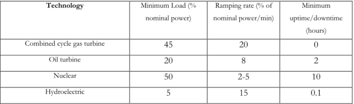
We assume no initial generation capacities in order to better disentangle the impact of each worst-case trajectories on investment decisions. For convenience, we further assume that no investment occurs in hydroelectric production units and keep the number of EVs to 0. As only one region is considered, transmission constraints and transmission costs are not included in the estimated model. Moreover, we constrain the variable for capacity investment to take only discrete values for nuclear, gas turbines (GT) and combined cycle gas turbine plants (CCG), and continuous values for other production and storage technologies. Nuclear investment is performed by blocks of 1.6 GW, corresponding to the rated power of the EPR Flamanville plant (the most recent nuclear power project in France), while CCG investments are made by blocs of 0.45 GW, which corresponds to the average nominal power of General Electric’s 9HA.01/.02 gas turbine. Finally, GT investments are performed by blocks of 0.3 GW. Flexibility characteristics of main generation units can be found in Table 1. Oil and gas prices are forecasted using
19
linear regression, we take Netherlands TTF and OECD countries CIF per million Btu dollar prices as reference on the period 2005-20181. Finally, we take a 5% discount rate and a CO2 price equal to 50€/ton,
without taking any CO2 emission ceiling. Investments decisions are made for the year 2021.
Technology Minimum Load (% nominal power) Ramping rate (% of nominal power/min) Minimum uptime/downtime (hours)
Combined cycle gas turbine 45 20 0
Oil turbine 20 8 2
Nuclear 50 2-5 10
Hydroelectric 5 15 0.1
Table 1: Flexibility characteristics of main generation technologies.
Sources: Gonzalez-Salazar et al. (2018), IAEA (2018), Schill et al. (2016), IEA (2015), Schröder et al. (2013),
EC JRC (2010).
In order to simplify the practical application of the methodology presented in section II, we use the theoretical worst-case joint state of nature ( ) instead of the empirical one ( ̂ ̂ ). Yet, this assumption may generate trajectories significantly more variable than empirically observed ones, which may lead to overly conservative investment decisions. Thus, we compare the results using residual demand trajectories generated using Algorithms 1 and 2 with empirically observed worst-case residual demand trajectories. For convenience, we let the reader refer to the Appendix for detailed explanations on the estimation of empirically observed worst-case trajectories.
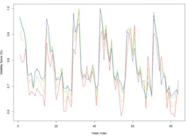
When considering the technical characteristics of generation technologies presented in Table 1, one actually notice that ramping rates are high enough for each technology units to vary their output within their entire production range. Indeed, as the model is defined using hourly time step, nuclear plants may vary their production by up to 100% of their rated power within an hour. Thus, ramping constraints are not binding within hourly time resolution. Moreover, when looking at dispatch data from RTE, it appears that nuclear plants especially are operated with much less flexibility than their technical characteristics actually allow. Taking national hourly production data on the period 2013-2018, Figure 1 shows the distribution of the rate of variation of nuclear output, defined with respect to nominal power:
20
Figure 1: Percentile distribution of the hourly rate of variation for nuclear power (right)
Note: The distributions are reported for each season as RD patterns change seasonally. Blue, red orange
and green respectively correspond to distributions for winter, spring, summer and autumn. The horizontal axis corresponding to percentiles of the distribution of variations.
It appears from Figure 1 that in roughly 90% of cases, nuclear output hourly variations are comprised within -2.1% and +2.1%. If we take the whole distribution, the lower an upper bounds on hourly variations observed in the data become -12.4% and +13.9%. Still, these figures remain largely inferior to the ramping capacities of nuclear units, which suggests they are operated in a much rigid way considering their flexibility characteristics. This directly relates to the fact that RTE2 uses nuclear plants for baseload
production instead of load-following.
A similar reasoning may be carried out for all technologies. We here focus on the case of nuclear, and add these operational “rules” as constraints to our optimization model. In order to precisely analyze how operational flexibility affects investment decisions, we include the minimum and maximum hourly variation values as operational bounds for thermal units.
21
III.3. Numerical simulation results
We start by analyzing the investment results obtained when using trajectories obtained using both Algorithms 1 and 2, that are presented in Table 2. As we assume no initial installed capacities, the figures reported correspond to the level of generation capacity for each technology in 2021, using successively theoretical worst-case RD trajectories and empirical trajectories. For each column, the figures on the left correspond to the optimal investment level with maximum-level-robust only decisions, while figures on the right correspond to both maximum-level-robust and variability-robust decisions. We provide in Appendix optimal investment results when taking simultaneously minimum-level-robust, maximum-level-robust and variability-maximum-level-robust decisions. As the variability of solar and wind capacity factors would have no effect on the shape of residual demand for null installed capacities, we impose various thresholds values for the level of investment in renewable technologies.
> 1 GWe > 3 GWe > 5 GWe
TT ET TT ET TT ET
Combined cycle gas turbine 4.05/8.1 4.95/5.85 4.05/9.9 4.95/6.75 4.05/10.8 5.85/6.75 Gas turbine 1.2/1.2 1.2/1.8 1.2/0.6 0.9/2.4 1.2/0.9 0.9/2.1 Nuclear 19.2/12.8 17.6/16 19.2/11.2 17.6/14.4 19.2/9.6 16/14.4 Wind 0/0 0.52/0 0/0 0.064/0 0/0.33 0.30/1.07 Utility-scale PV 1/1 1.21/1 3/3 2.93/3 5/4.67 4.70/3.93 Commercial PV 0/0 0/0 0/0 0/0 0/0 0/0 Residential PV 0/0 0/0 0/0 0/0 0/0 0/0 Battery storage 1.40/9.89 3.70/2.73 2.41/10.40 5.51/6.40 2.89/10.73 6.55/3.50
Table 2: Optimal investment level by technology, with constraints on minimum installed capacities for renewables (TT= Theoretical trajectories only)
It can first be noted from Table 2 that as the threshold for renewables installed capacities increases, the investments in peaking technologies (CCG and gas turbines) are non-decreasing for all cases, while the capacities in nuclear decrease. Yet, while in the level-robust only case, investment in peaking technologies remain constant with respect to the threshold value, the sum of their installed capacities is always increasing with level-variability robustness (especially using theoretical trajectories). The behavior of investment in batteries is more chaotic: as its optimal level steadily increases both for level-robust only and level-variability-robust investment decisions using theoretical trajectories, its level-robust capacities increase while its level-variability-robust capacities decrease using empirical trajectories.
22
When hedging against both types of worst-case trajectories, peaking technologies and battery storage seem to behave as substitutes in the empirical case and complements in the theoretical case. This complementarity can be explained by the fact that, while higher capacities in battery storage allow the smoothing of highly variables renewable production when capacities increase, thermal peaking technologies remain necessary as the capacity factors of wind and solar units is quasi null in the level-maximizing RD trajectory. Theoretical trajectories may thus result in slight over conservatism compared to empirical ones. Indeed, as level-robust only investment levels obtained using theoretical and empirical trajectories are quite close, this indicates level-maximizing trajectories have similar profiles while the theoretical variability-maximizing trajectory exhibits significantly higher variability than the empirical one. High storage capacities are thus necessary for high variability periods, yet the equilibrium of the electric system still requires significant thermal capacities for high residual demand periods.
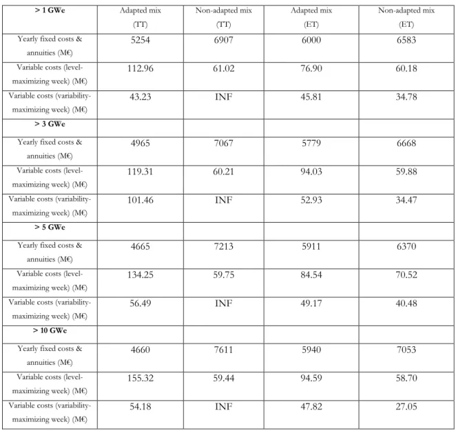
> 1 GWe Adapted mix (TT) Non-adapted mix (TT) Adapted mix (ET) Non-adapted mix (ET) Yearly fixed costs &
annuities (M€)
5254 6907 6000 6583
Variable costs (level-maximizing week) (M€)
112.96 61.02 76.90 60.18
Variable costs (variability-maximizing week) (M€)
43.23 INF 45.81 34.78
> 3 GWe Yearly fixed costs &
annuities (M€)
4965 7067 5779 6668
Variable costs (level-maximizing week) (M€)
119.31 60.21 94.03 59.88
Variable costs (variability-maximizing week) (M€)
101.46 INF 52.93 34.47
> 5 GWe Yearly fixed costs &
annuities (M€)
4665 7213 5911 6370
Variable costs (level-maximizing week) (M€)
134.25 59.75 84.54 70.52
Variable costs (variability-maximizing week) (M€)
56.49 INF 49.17 40.48
> 10 GWe Yearly fixed costs &
annuities (M€)
4660 7611 5940 7053
Variable costs (level-maximizing week) (M€)
155.32 59.44 94.59 58.70
Variable costs (variability-maximizing week) (M€)
54.18 INF 47.82 27.05
Table 3: Cost decomposition of the electricity mix, with constraints on minimum installed capacities for renewables (INF= Infeasible dispatch, TT only)
23
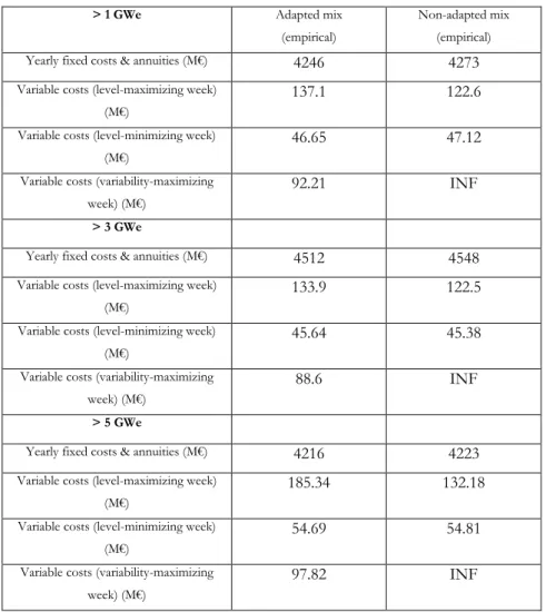
As shown in Table 3, the adapted mix, corresponding to level-variability robust investment decisions, systematically exhibit lower yearly fixed cost and annuities than the non-adapted mix, corresponding to the level-only robust decision. Similarly, the adapted mix always has higher variable costs, both in the case of the level-maximizing and variability-maximizing weeks, compared to the non-adapted one. However, the theoretical variability-maximizing week is always integer infeasible with the non-adapted mix, even when allowing curtailment of renewables and load shedding, which would result in a system blackout. Yet, the empirical variability-maximizing week remains feasible with the non-adapted mix and at least cost than with the adapted mix. Apart from the theoretical case, we observe a clear trade-off between high variable costs and low fixed costs mixes depending on targeted level of system flexibility.
Yet, both adapted and non-adapted mixes exhibit a high share of CO2 emitting production capacities, which would result in highly polluting and expensive mixes depending on the price of carbon. After measuring that a higher CO2 price doesn’t significantly change the above results, we impose a restriction
on the maximum number of oil and gas power plants in the mix. This ceiling is defined such that
the optimization problem is infeasible for any number of fossil plants strictly lower than . In other words, corresponds to the minimum number of oil and gas production units necessary to maintain the frequency of the electric system within acceptable bounds without using reserves. The resulting production mixes and cost decomposition are presented in Table 4 and Table 5 respectively
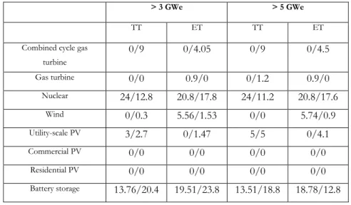
> 3 GWe > 5 GWe
TT ET TT ET
Combined cycle gas turbine 0/9 0/4.05 0/9 0/4.5 Gas turbine 0/0 0.9/0 0/1.2 0.9/0 Nuclear 24/12.8 20.8/17.8 24/11.2 20.8/17.6 Wind 0/0.3 5.56/1.53 0/0 5.74/0.9 Utility-scale PV 3/2.7 0/1.47 5/5 0/4.1 Commercial PV 0/0 0/0 0/0 0/0 Residential PV 0/0 0/0 0/0 0/0 Battery storage 13.76/20.4 19.51/23.8 13.51/18.8 18.78/12.8
Table 4: Optimal investment level by technology, with constraints on minimum installed capacities for renewables and maximum on CO2 emitting power plants
While CO2 emitting technologies completely disappear from the non-adapted mixes, both for theoretical and empirical trajectories, Table 4 exhibits much higher battery storage capacities for adapted mixes compared to Table 2, with an incompressible level of oil and gas plants only slightly lower than for unconstrained investment. With a minimum level of 3 GWe of renewable capacities, the TT adapted mix
24
has 96 % higher battery storage capacities while roughly 16% lower oil and gas production capacities compared to Table 2, while these ratios to expand to 372% and 56% respectively for the ET adapted mix. A similar observations can be made when imposing a minimum of 5 GWe of renewables in the mix. The flexibility “loss” of not investing 1 GWe of oil or gas production unit in the system must be compensated by more than 6 GWe of battery storage to ensure an equivalent level of system flexibility.
As observed in Table 5, this results into significantly higher yearly fixed costs and annuities for both adapted and non-adapted mixes. For a threshold of 3 GWe, TT and ET adapted mixes respectively exhibit 15% and 24% higher yearly FOM costs and annuities compared to Table 3, while these ratios decrease to 13% and 18% respectively for a threshold of 5 GWe of renewables.
> 3 GWe Adapted mix (theoretical) Non-adapted mix (theoretical) Adapted mix (empirical) Non-adapted mix (empirical) Yearly fixed costs &
annuities (M€)
5718 8675 7189 8401
Variable costs (level-maximizing week) (M€)
103.30 25.17 55.20 38.83
Variable costs (variability-maximizing week) (M€)
37.25 INF 29.66 INF
> 5 GWe Yearly fixed costs &
annuities (M€)
5283 8802 7006 8409
Variable costs (level-maximizing week) (M€)
129.54 25.15 55.52 33.98
Variable costs (variability-maximizing week) (M€)
95.61 INF 30.24 INF
Table 5: Cost decomposition of the electricity mix, with constraints on minimum installed capacities for renewables and maximum on CO2 emitting power plants
Similar conclusions can be drawn when comparing maximum-level-robust to minimum-maximum-level-robust and variability-robust decisions with empirical data. Investment results and costs figures are reported in Table 6 and 7 in Appendix. However, we made the assumption that there are no initial capacities. In the case preexisting capacities are not retired when new investments are made, increasing the share of renewables in the electric mix increases more than proportionally the total FOM costs and annuities of the system. As increasing decarbonization imposes increasingly avoiding CO2 emitting technologies, the total costs of the system will increase more rapidly than the share of renewables because of increasing investments in storage for flexibility requirement. In the case the electric mix is not properly designed in terms of flexibility needs (non-adapted mix), the objective of minimizing CO2 emissions while developing renewables may trigger infeasible situations resulting in system blackouts with extremely high costs for the society.
25 IV- Conclusion
We presented in this paper an original approach based on philosophy of DRO and the tools of RO in order to derive worst-case trajectories of uncertain parameters, derived both in terms of level and variability. As a higher share of renewables in the electricity mix is associated with higher residual demand variability, it makes sense to hedge against situations that would require high flexibility from the system and push power plants to their technical limits.
For each possible matrix of quantile values for the uncertain parameter defined in the trajectory ambiguity set, we derive its level-maximizing and variability-maximizing trajectories expressed in quantiles of its empirical distribution. For each value of this matrix, it is possible to derive a pair of trajectories and thus a joint distribution of worst-case trajectories associated to each possible value of the vector described in Section 2. We leave the derivation of the worst-case theoretical probability distribution of the uncertain parameter based on this joint distribution for further research. Still, we prove how our simple framework can be used for refining utility investment decisions in the context of the transition of electric systems, allowing us to derive optimal solutions hedging against situations of extremely levels and variability of uncertain parameters at minimum cost.
26 Appendix:
Appendix to III.1.:
The presentation and formulation of variables, parameters and equations is largely borrowed from De Sisternes (2013), as it provides great readability to the model and facilitates the understanding of equations.
III.1.1. Indices and sets
, where is the set of electricity generation technologies , where is the subset of thermal generation technologies , where is the subset of wind power generation technologies , where is the subset of solar generation technologies
, where is the subset of storage technologies , where is the set of geographical regions , where is the set of years
, where is the set of seasons , where is the set of hours
, where is the set of worst-case trajectories
The sets used in the model can be classified into two types: sets and subsets related to production and storage technologies and sets related to various temporal and geographical scales. corresponds to the set of available generation and storage technologies that can be built. It can be decomposed into subsets, each corresponding to varieties of technologies: and respectively denote wind and solar generation technologies , while refers to the subset of thermal power units, including in our case combined cycle gas turbines (CCGT), fuel turbines, coal and nuclear technologies.
corresponds to the set of hours in a week as we model investment and dispatching decisions with an hourly time resolution. Our model thus combines multiple time scales in order to both account for long-term and short-long-term constraints which delong-termine investment and dispatching decisions. As we model cyclical stochastic processes, the distributions of parameters and are identical. Note that when referring to the distribution of , we actually refer to the distributions of { } .
27
III.1.2. Parameters
: residual demand for trajectory in region , year , season and hour [MW]
: investment cost for technology in year [€/MWe]
: annuity paid for investment in technology made in year [€/MWe/year]
: annual fixed operation & management costs for technology in year [€/MWe]
: variable cost for technology in year [€/MW]
: start-up cost for technology in year [€]
: investment cost for a transmission line in year [€/km]
: annuity paid for investment in a transmission line made in year [€/km/year]
: annual fixed operation & management cost for transmission line in year [€/MW] : value of lost load [€/MW]
: initial capacity level for technology in region [MWe] : initial transmission capacity between regions and [MW]
: maximum output level for production technology [%] : minimum stable power output level for technology [%] : maximum ramp-up capability for technology [MW/h] : maximum ramp-down capability for technology [MW/h]
: minimum up-time for technology [h] : minimum down-time for technology [h]
: CO2 emissions per unit output for technology [ton/MW] : round-trip efficiency for storage technology [%] : maximum state of charge for storage technology [%] : minimum state of charge for storage technology [%] : round-trip efficiency for electric vehicles [%]
: maximum state of charge for electric vehicles [%] : minimum state of charge for electric vehicles [%]
: average distance driven between hours and [km]
: per kilometer electric consumption of electric vehicles [MW/km]
: total number of vehicles in region and year
: share of electric vehicles in total vehicle fleet in region and year [%] : distance between the centroids of regions and [km]
28 : price of CO2 carbon ton in year [€/ton]
: discount rate [%]
: additional transmission capacity for each new transmission line [MW]
: slack parameter
: frequency primary control tuning parameter : frequency deviation absolute limit
As our model allows investment in transmission capacity, cost parameters can be divided between generation costs (investment costs expressed in annuities, maintenance costs, variable and start-up costs) and transmission network costs (investment costs expressed as annuities, maintenance costs). We make the assumption that the variable cost of transmitting electricity is equal to zero. Finally, we define the value of lost load (VOLL), which corresponds to the cost of one non-served unit of electricity demand. We introduce generation units technical constraints, including maximum and minimum stable power output (the latter applying when a unit is online, ie effectively feeding electricity into the network), ramping up and down limits and minimum up and down times, in addition to CO2 emission rate, for each technology. Specifically for storage technologies and electric vehicles (EV), we consider maximum and
minimum state of charge limits, charging speed, round-trip efficiency (we choose ), in
addition to the average number of kilometers for each time interval of the day in order to approximate the electricity consumption requirements of an EV fleet.
Finally, we introduce distance measures for each arc , where its length is calculated as the distance in kilometers between the centroids of regions and . This provides an approximation for the length of new transmission lines to build for reinforcing transmission capacities along arc . Yet, we may consider the resulting investment costs as upper bounds as centroid distance is likely to overestimate the length of new lines needed to link the two regions.
III.1.3. Variables
: investment level in technology in region and year [MWe]
: investment in new transmission lines between regions and in year [MW]
: installed capacity of technology in region and year [MWe]
: transmission capacity between regions and in year [MW]
: output power of generation technology plants in region , year , season and hour of the week [MW]