Record Number: 460
Author, Monographic: Couillard, D.//El Sabh, M. Author Role:
Title, Monographic: Étude des répercussions sur l'environnement marin du projet Ashland Oil Terminal Translated Title:
Reprint Status: Edition:
Author, Subsidiary: Author Role:
Place of Publication: Québec Publisher Name: INRS-Eau Date of Publication: 1973 Original Publication Date: Volume Identification: Extent of Work: vi, 98 Packaging Method: pages Series Editor:
Series Editor Role:
Series Title: INRS-Eau, Rapport de recherche Series Volume ID: 46
Location/URL:
ISBN: 2-89146-049-9
Notes: Rapport annuel 1973-1974
Abstract: Rapport rédigé pour Ashland Oil Canada Ltd 15.00$
Call Number: R000046 Keywords: rapport/ ok/ dl
Etude des répercussions sur l'environnement
marin du projet Ashland Oil Terminal
~r
D. Couillard, M. El Sabh
INRS-Eau
Université du Québec
C.P. 7500, Sainte-Foy
Québec G1V 4C7
RAPPORT SCIENTIFIQUE No 46
Rapport rédigé pour
Ashland Oil Canada Ltd.
Etude des répercussions sur l'environnement
marin du projet Ashland Oil Terminal
~r
D. Couillard, M. El Sabh
INRS-Eau
Université du QUébec
C.P. 7500, Sainte-Foy
Québec G1V 4C7
RAPPORT SCIENTIFIQUE No 46
Rapport rédigé pour
Ashland Oil Canada Ltd.
ISBN 2-89146-049-9
DEPOT LEGAL 1973
Tous droits de traduction, de reproduction et d'adaptation réservés
Etude des répercussions sur l'environnement marin du projet "Ashland Oil Terminal"
Résumé
La première partie du rapport présente la description de l'état actuel des mouve-ments et de la circulation des masses d'eau, des marées, des glaces et l'état ac-tuel de la pollution de l'eau.
On
présente ensuite les influences et les réper-cussions de la construction du port et de la digue sur les variables citées pré-cédemment ainsi que sur l'apparence et l'esthétique de la région portuaire de Grande-Ile, Kamouraska.La deuxième partie du rapport décrit les méthodes actuellement utilisées pour la surveillance et le contrôle des fuites d'huile dans le milieu marin (spectro-ra-diométrie, analyse multi-spectrale, radar). La télédétection est un moyen simple, reproductible, précis et automatique pour évaluer la surface affectée par une fui-te d'huile, la nature et la quantité de polluant impliquée.
La troisième partie du rapport propose l'implantation d'un réseau d'acquisition des données de qualité (eau et sédiments) en deux étapes. La première pour é-tablir la qualité physique, chimique et biologique du nilieu; la seconde pour rationaliser le réseau
à
partir des données et de l'expérience acquises. Enfin, on propose une méthode d'évaluation de l'impact des opérations portuaires nomina-les sur la qualité des eaux du fleuve.Mots-clé:
impact, répercussion, environnement, marin, fleuve, eau, port, super-port, huile, pétrole, surveillance, contrôle, fuite, déversement, réseau, acquisition, donnée, qualité, Saint-Laurent, Grande-Ile, Kamouraska
Référence:
Couillard, D., El Sabh, M. (1973). Etude des répercussions sur l'environnement marin du projet "Ashland Oil Terminal". INRS-Eau, rapport scientifique no 46,
98
p.(Pour Ashland Oil Canada Ltd).
TABLE DES MATIERES
RESUME
11.1
1.2
1.3
1.4
1.5
1.6
1.7
EFFECTS OF GRANDE- ILE SUPERTANKER PORT AND JETTI ON THE MARINE
ENVIRONMENT OFF KAMOURASKA AREA
Introduction
Water Masses
Circulation
Tides and Sea Level
Tidal Flats
Ice
Pollution Concern
1.8 Construction of Kamouraska Port and Jetty and their Effects on
PAGE
i 2 2 6 11 20 3943
48Marine Environment
51
1.9 Bibliography
54
2 33.1
3.2
3.3
3.4
3.5
3.6
4AFP ARENCE DES INSTALLATIONS POR1UAIRES DE GRANDE- ILE, KAMOURASKA
PROCEDURE DE SURVEILLANCE ET DE CONTROLE DES FUITES D' HUILE
Introduction
Spectro-radiométrie
Analyse multispectrale
Radar
Conclusion
Bibliographie
IMPLANTATION D'UN RESEAU D'ACQUISITION DES OONNEES DE QUALITE
4.1 Problématique
4.2 Description du réseau
i i63
67
67
6873
81
83 84 86 86 874.2.1 Première étape 87
4.2.2 Seconde étape 88
4.3 Description de l'échantillonnage d'un site 89
5 METHODE D'EVALUATION DE L'IMPACT DES OPERATIONS PORTUAIRES NOMINALES
SUR LA QUALITE DES EAUX DU FLElNE 92
5.1 Implantation du réseau d'acquisition de données 92
5.1.1 5.1. 2 5.1. 3 5.1.4 5.1. 5
Simulation des pertes dans les opérations portuaires 93
Description de l'environnement susceptibles d'être affectées
par les opérations portuaires 93
Evaluation de la qualité des eaux dans la région portuaire 94
Choix des stations fixes 94
Echantillonnage complémentaires 95
5.2 Mode d'échantillonnage 95
LISTE DES FIGURES
PAŒ
1
Gulf of St. Lawrence
3
2
Lower St. Lawrence River and Estuary
53
Salinity and temperature on north and south of channel
84
Distribution of surface salinity
95
Distribution of surface tempe rature
106
Current velocities in Cabot Strait
127
Current velocities
inthe St. Lawrence Estuary
128
Typical summer surface circulation pattern in the Gulf of
St.Lawrence
159
Autumn surface circulation
inthe Gulf
on St. Lawrence
16
10
Field of the surface geostrophic currents in the Gulf of St. Lawrence
17Il
Tidal constituent M
2 21
12
Tidal constituent KI
2213
Regions and cross-sections of the St. Lawrence River and Estuary
showing tide gauge locations
2414
Daily sea level at Trois-Rivières
3215
Daily sea level at Quebec
33
16
Daily sea level at Pointe au père
3317
Monthly mean level
inthe St. Lawrence Estuary
35 18Monthly deviation from the mean level Upper St. Lawrence
36 19Monthly deviation from the mean level Lower St. Lawrence
3720
Five year mean ice concentration
4421
Apparence d'un port super-pétrolier
àGrande-Ile, Kamouraska
6522 Rayonnement solaire au niveau du sol
23 Distribution spectrale du rayonnement diffus sous différents
angles
24 Degré de polarisation en fonction de la position du soleil
25 Détection et identification des huiles par fluorescence
26 Rayonnement en fonction de l'épaisseur d'huile
27 Schéma décrivant la méthodologie de l'implantation du réseau
v
69
70 71 74 7696
LISTE DES TABLEAUX
PAGE
l
Characteristics of the entrances to the Gulf of St.Lawrence
4
IIa Harmonie constituent M
2 (EST)
25
IIb Harmonie constituent S2
(EST)
26
Ile Harmonie constituent N
2 (EST)
27
IId Harmonie constituent K
1 (EST)
28
Ile Harmonie constituent 01
(EST)
29
IIf Harmonie constituent M4
(EST)
30
IIg Harmonie constituent MS4 (EST)
31
III Description of the tida1 marshes of the south shore of the
St.Lawrence Estuary
41
1 Effects of GRANDE ILE Supertanker Port and
Jetty of the marine environment of Kamouraska
area
1 EFFECI'S OF GRANDE-ILE SUPERTANKER PORI' AND JETrY
ON THE MARINE ENVIRONMENT OFF KAMJURASKA AREA 1.1 INTRODUCI'ION
2 •
It is pe:r:haps enlightening, before delving into the proposed hamor and Jetty at Grande Island, Karrouraska, and their effects on the environnent, to review our knCMledge on the physical oceanography of the St. Iawrence Gulf and Estuary.
Canadian hydrographic charts carry the narre "St. Lawrence River"
eastward to a sectio n passing roughly through the centre of Anticosti Island, and the narre "Gulf of St. Lawrence" for the renainàer of the system bounded by the mainland, Cape Breton Island, and Newfoundland
(Fig. 1). Sinee the upstream limit of salt penetration is near Quebec City, the tenn "estuary" could, by Pritchard' s (1952) defini tion, be used to include all of the river and gulf belCM this point. In this report the tenn "river" is used here te refer to the area above Quebec City, the "estuary" between Quebec City and Pte. des Monts, and the
"gulf" belCM Pte. des Monts. This use of the ward "estuary", following Forrester (1967), is admitted1y an ~dient te bridge the ill-àefined boundary between the regions bearing the historically accepted narres "St. Lawrence River" and "Gulf of St. Lawrence".
3
The Gulf of St. Lawrence has an area of 24lx10 sq. km. (Forrester and Vandall, 1968). Through the St. Lawrence River and nurœrous smaller ri vers the gulf recei ves the drainage f:rom an area of approximately l3x105 sq. km. It is the principle sea access to our largest cilies and
te - over 60% of the population of Canada, and i t is the source of lIDre than 40% of all Canadian sea-fish landings.
The physica1 features of the Gulf have been sumnarized by El-Sabhètàl. (1969) who mention all the published and unput:>lished li terature of
- - - - -GASPÉ PEN. QUEBEC NEW BRUNSWICK 1
L ...
~...
...-.!:.""H*=-1'=====-=-::.-::::::.::=== .. ---Fig. 1. QUE BEC GULF OF ST. LAWRENCE ~AGOAlENt:,.
ISLANDS Gulf of St. Lawrence 1 '1 1 , 49[ NEWFOUNDLAND 1 i 1 48\ , : l' " North~
-1
(3 1 1 1 1 OCEAN .1 1,,~.I
4 .
physical oceanography up to 1968. To quote from that paper: "The principle cormection with the Atlantic Ocean is through cabot Strait. A nore restricted cormection is through the Strai t of Belle Isle. The Strai t of Canso, separating the mainland of Nova Sootia from Cape Breton Island, is very nar:row and since 1954 has been closed, except for a lock through the causeway. Table 1 shows the
characteristics of these cormections ot the Gulf.
rAB LE 1
Characteristics of the entrances to the Gulf of St. Lawrence
~ Cabot Estuary sec- Belle Canso Strai t
Strait tion (Poin te Is le oefore
des Monts) Strait causeway
Minimum width 104 km. 45 km. 16 km. l km. Maximum unrestricted 480 m. 330
m.
60 m. 35 m. depth Minimum cross-section 35 x 106 m2 12 x 106 m2 1 x 10⁶ m2 25 x 103 m2 area after cause-way 25 m. 10 m. 250 m25 •
The main feature of the bathymet:ry of the Gulf is the Laurentian Channel (Fig. 1) extending fran the Continental Shelf south of Newfoundland through the gulf nearl y to the nouth of Saguenay River. From the edge of the Continental Shelf to cabot Strait i t has depths ranging approxirnately fran 600 to 400 m. Fran cabot Strait inward to a distance of about 640 km. i t has depths of 400 to 300 m. The Esquiman Channel, branching off fram the Laurentian Channel, extends fram the central portion of the gulf northeastwards tCMards the Strait of Belle Isle. It is nore than 180 m. deep except as i t approaches· the strai t. To the south of the Laurentian Channel is the shallCMer area knCMl1 as the Magdallen ShallCMs. The estuarine Channel,
as shCMl1 in Fig. 2, is a furmel-shaped bay, va:rying in width fram
20 km above the nouth of the Saguenay River to 45 km near pte. des Monts. The depth increases fran about 10 m in the shoal area off Quebec City to 60 m above the Saguenay. Off the nouth of this river, the bed drops abruptly to 300 m, and remains approximately at this depth through the rest of the defined system.
. _. '_'-'~-'-'-'_'gQm
6 •
1.2 ~R MASSES:
Al though the water mass pattern in the Gulf shONS a three-layer
structure in sumœr, the basic pattern exhibi ted in winter, when there is a cold upper layer vcuying in thickness from 100 to 150 m. with terrperatures as ION as -1. 70 C and salinities vcuy between
32.5 and 33
0/00.
This is underlain by the deep water extending to the bottan of the Laurentian Channel, wi th temperatures between 4 and 60 C, and salinities close to 34.50/00.
The cold layer contracts rrarkedly in volmre in spring and surnrœr as the upper water is heatedby the sun and freshened by the spring land drainage, so that a third layer appears at the surface, extending dCMIl to sone 50 to 75 m., with terrperatures as high as 180 C and salinities as low as 260
/00.
Originally the cold water at intennediate depths was thought to originate outside the gulf, but is nON believed to be nostly locally
forrœd during the winter. From a quanti tati ve terrperature - Salini ty study of the gulf, Forrester (1964) concluded that " the interrœdiate cold-water layer may be canpletely accounted for as the rerrn.ant of the locall y-forrœd upper mixed layer of the winter. Wi th the advent of spring the :rœlting of ice and the increase in nm-of;E would decrease the salini ty and the surface wanning would increase the terrperature at the surface. These effects would then be diffused downwards by
vertical mixing, leaving a terrperature minimum near the bottom of the original mixed layer". Recent inte:rpretation of the oxygen observations in the gulf (D'Anglejan and Dunbar, 1968) and the existence of a sumœr oxygen rnaxirnum tONards the bottom of the therrrocline just above the interrœdiate layer, support Forrester' s view about the origin of this layer.
By study of the terrperature-salinity relationships., Lauzier and Bailey (1957), follONing McI.ellan (1957), concluded that the deep wann waters are forrœd outside the gulf through a mixing of Labardor and Slope waters.
7 .
Lauzier and Trites (1958) shCM that these deep waters have a maximum
terrperature at a salinity of 34.6
0/00.
Variation of the maximumte:rrq:Jerature fran a lCM of about 40 C in the 1920' s te a high of about 60 C in the earl y 1950' s, aecorrpanied by an increase in volurœ of the
deep layer, was abserved. This wanning period was followed by a cooling trend up to 1967, where terrperatures decreased to 40 C, although wanning beeame apparent agin fran 1967 to 1971 (EI-Sabh, 1972).
Onl Y few investigations were carried out in the St. Lawrence Estuary to study variations of the oceanographie properties. In February and May 1963, Neu (1970) carried out a detailed study between Quebee City and Pte. des M:>nts. These two rronths were chosen prirnaril y to penni t an evaluation of the differences which occur in the estuary due to a large variation in the fresh water inflCM. It was coneluded from this study that in the deep section of the St. Lawrence Estuary, the water is di vided into two layers, an upper and a deep layer, while in the shallCM section the upper layer extends throughout the depth. The
salini ty of the deep layer was the same in May as in February, suggesting that its content remains constant throughout the year although the
salini ty of the upper layer changes wi th the fresh water inflCM. The
upper layer is triangular in cross-section wi th the deeper side along the south shore where the water is principally fresher, but colder in February and wanœr in May (Fig. 3) than on the north shore side, except where the Saguenay River enters the system. The depth of this layer inereases seaward along the south shore while decreasing along the north shore ~ Figure (4) shows horizontal distribution of surface salinity in February, May and July, while surface temperature in the first two nonths are shCMl1. in Fig. (5).
9 Metre Otpfl\ ORLEANS ISLAND 9 Metre Oepth ORLEANS ISLAND 70° \6dO Pol"le-dt!~-Monh i 49° '8
.
47 9 • (a) (b) (c) Fig. 49 Metr. Depth [ St. Lowrence River Inflo," 8200m~S Q -O(-~)-ORLEANS ISLAND 9 Metre Depth ORLEANS ISLAND S . ~OUP Inflo. 710 1ft 3/5 \~0Cl""""'Y Rove, ,"flO" 710m3/S
ITADOUSSA~
-~~&
POINTE DES~
---t
MONTS----t-",
-US)_ -... ... ---(-I)~--, ---....~(.,)-
.... e f'ATHER POINT 10 •Pig. 5 distribution of surface tenperature in {a) Februaxy 1963 ana.
(b) May 1963, (After Neu, 1970).
fa)
Il •
1.3 CI~ION:
'!he genera1 circulation aIOund the Gulf of St. Lawrence is anti-c1ockwise. Infonnation on the circulation has been àeduced fram direct current Ireasurerrents (Fa.r:quharson, 1962, 1963, 1966; B1ackford, 1965, Forrester, 1967, and Lawrence, 1968 ); fram
dynarnical calculations (MacGregor, 1956; Trites, 1963, Farquharson, 1963, 1966; B1ackford, 1965, 1967; Farquharson and Bai1ey, 1966; Forrester, 1967; E1-Sabh and Joharmessen, 1972); fram drift bott1es and drogue studies (Burrpus and Lauzier, 1965; Lauzier 1965, 1967; Boudreault and Héritier, 1971, Boudreault, 1972); and fram t:heoretical
rroàe1s (B1ackford, 1965; Murty and Taylor, 1970). The
bulk of investigation has been done during the ice-free nonths of the year, and very 1itt1e infonnation is avai1ab1e for the winter rronths.
Ea:téIy circulation studies in Cabot Strai t were œxried out by Dawson (19.1:3 .. ) and Sandstrom (1919). Fran geostrophic calculations
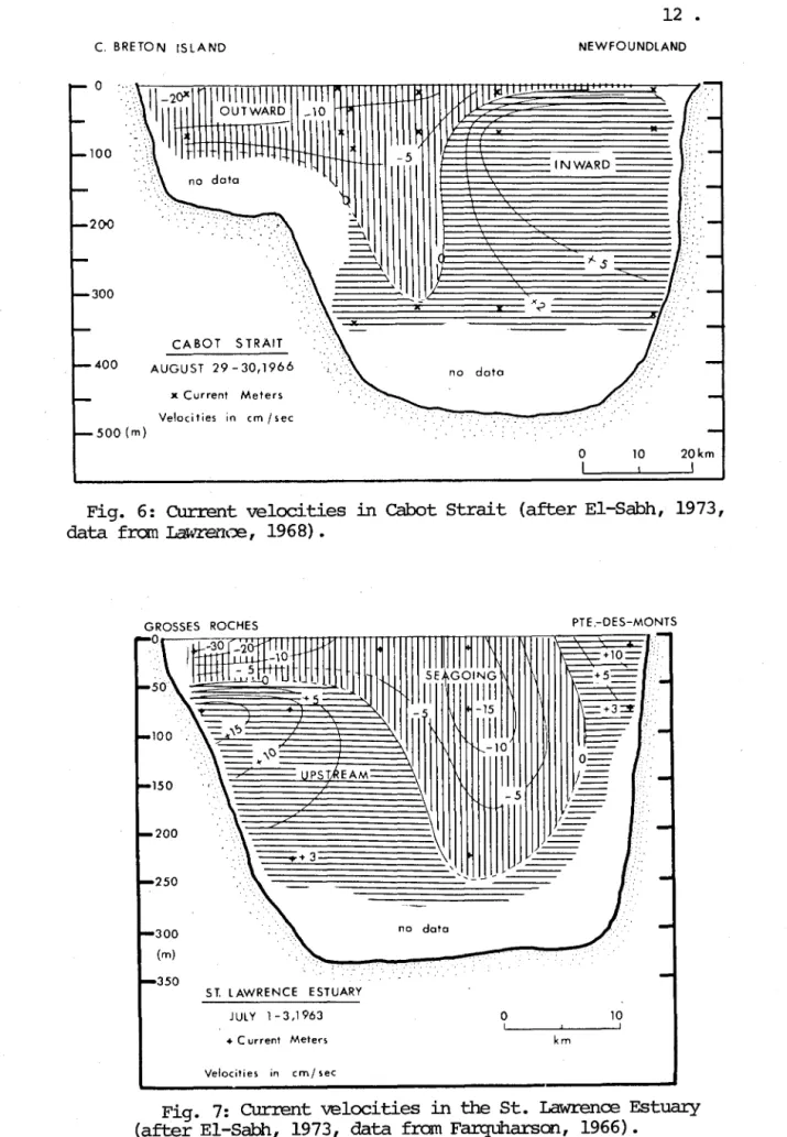
MacGregor (1956) found the circulation in the strai t to be marked by an outward surface fION strongest on the cape Breton side wi th a tendency for a weak inf10w along the Newfoundland side. He found much variation fran cruise to cruise, wi th strongest currents in August and 1east in April and May. In recent years direct current Ireasurerrents have been undertaken across Cabot Strai t for approximate1y one nonth. An examination of these Ireasurerrents (Fig. 6) suggests an inf10N through the who1e depth of the Newfoundland side of Cabot Strai t.
(E1-Sabh, 1973) Investigation in Belle Isle Strait was.undertaken by Dawson (1907);
Huntsman, Bai1ey and Hachey (1954); Bai1ey (1958), and Farquharson and Bai1ey (1966). These studies al1 indicate that a1though there is no large net f10W' through the strait, there isan inward noverrent of Labrador coastal water on the Labrador side and an outf10W' of the gulf water on the Newfoundland side. On sare occasions a strong out fION
12 .
C. BRETON ISLAND NEWFOUNDLAND
o 100 200 300 400 CABOT STRAIT AUGUST 29-30,1966 x Current Meters Velocities in cm /sec -5 1 no data 500 (m) o 1 10 20km 1
Fig. 6: CUrrent ve10cities in cabot Strait (after E1-Sabh, 1973, data fram Lawrence, 1968).
GROSSES ROCHES PTE ,-DES-MONTS
°r-~~mmnrrmnmmnmmrrmmwm~mmrrm~~~~ ST. LAWRENCE ESTUARY J UL y 1 - 3,1 963 + C urrenl Melers Velocilies in cm/ seC no data GOII\IG 1111 -15
III
-10Il
-5 , _ _~j
,
o 10 '-,---'---, kmFig. 7: CUrrent ve10ci ties in the St. Lawrence Estuary (after E1-Sabh, 1973, data fram Farquharsan, 1966).
13 •
through the strai t is observed to 1ast for several days or even weeks, mile on ether occasions strong inf10w may dorninate for an equa11y
long tille. The possible causes of these ternporary dominant f10ws are suggested to be the north-south bararetric pressure gradient and the wind effect (Dawson, 1907; Bai1ey, 1958; and Lawrence, 1968).
Prior to the construction of the Canso causeway there was a fair1y strong current through the Strai t of Canso fram ~rge Bay towards the Atlantic Ocean. Since the strai t was c10sed this current has been
rep1aced by a fair1y strong north-easter1y outset along the shore of
Cape Breton Island tCMards Cabot Strait.
The outf1ow fram the St. Lawrence River, which is the source of over ha1f of the fresh water discharge into the gulf, has a major influence on the circulation of the Gulf of St. Lawrence. Farquharson (1966) and Forrester (1967, 1970), have reported on current Iœasurerœnts made in the St. Lawrence Estuary. By IroOring strings of water bott1es and
tripping them by tllne' re1ease, Forrester was able to obtain simul taneous observations through the cross-section of the estuary near pte au Père. E1even sets of simll taneous observations were obtained each at a different phase of the semidiurnal 1unar tide. Corrparison of geostrophic currents
wi th direct current observations showed that a tidal oscillation was present in the vertical shear of the geostrophic current in response to the vertical shear in the tida1 streams. It was conc1uded fram this that Iœaningful geostrophic current in the estuary can on1y be detennined fram averaged tille series observations. Forrester and E1-Sabh (1972) show how geostrophic currents adjusted to satisfy the condition of zero average salt transport fai th full Y produce accurate estimates of fresh water discharge fram the St. Lawrence Gulf and Estua:ry. It was estimated that horizontal advection is rrore inportant than horizontal diffusion as a transport process.
14 •
A fairly oonsistent feature observed in the outflow of the estuary is the Gaspé current, which begins to develop in the RiIrouski -Pte. des M:::mts areas (Fig. 7) and extends throughout the entire
length of the Gaspé ooast. This current is ooupled wi th an inflow on the Antioosti Island side of Gaspé Passage. This general pattern., however, is subject to oonsiderable variations and the Gaspé current may on occasions disappear (Fa:rquharson, 1966).
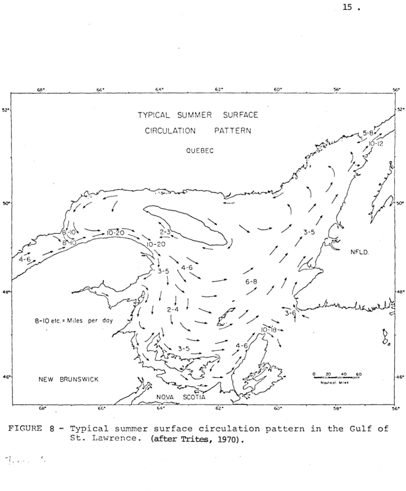
Utilizing all infonnation and :rœasurerœnts available in the gulf during surmer period, Trites (1970) was able to draw a typical surmer surface circulation pattern. (Fig. 8). The general two-way flow in bath entrance straits, the counterclockwise circulation in the interior part of the Gulf, and the Gaspé current are the daninant features. Highest speeds are found in the Gaspé current and in the outflow through cabot Strait, reaching values of 10-20 mi/day. From the nove:rœnts of parachute drogues in the southem gulf in surnœr and
by calculation of relative geostropic flow, Blackford (1965, 1967) distinguished both clockwise and anticlockwise gyres 20-30 km. in diameter in the layer above the thernocline. These smaller gyres were observed to nove with the general southeasterly flow along the north shore of Prince Edward Island.
During the last 20 years, a study of a network of stations in the Gulf of St. Lawrence was carried out during November of each year to
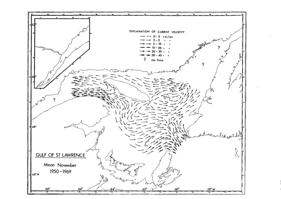
provide the terrperature-salini ty data wi th which the Ice Forecast Centre of the D.O.E. prepare their ice forecast. The bulk of this data provide an excellent opportuni ty to study the :rœan surface circulation pattern. during Noverrber (El-Sabh, 1973). The existence of two anticlockwise gyres, west and southeast of Anticosti Island, the Gaspé current with velocities between 30-40cm/sec, the inflow along the Newfoundland side of cabot Strai t and outflow along the Cape Breton side are the main features in the average autumn surface circulation (Fig. 9).
15 •
~ __ ~œ_' ____ ~ __ ~~~-' ____ ~ ____ 6~4' _ _ _ _ ~ _ _ _ _ 6~2_' _ _ ~~ _ _ ~60_' _ _ _ _ ~ _ _ ~~~' _ _ _ _ ~----~1·
TYPICAL SUMMER SURFACE
CIRCULATION PATTERN QUEBEC d
.~5-8~
~. /10-12 /" /)
'î /.-.
J
1
"-..
~--
)
NFLD . ./' ~ 6-8 4/
8-10 etc. = Miles per day
46"
NEW BRUNSWICK
0 ___ 20 40 60
=-=-(,(.. ~8'
FIGURE 8 - Typical summer surface circulation pattern in the Gulf of St. Lawrence, (after Trites, 1970).
-
[, , . ~. 48' 46' ~6' \.,GULF OF 51 LAWRENC E
Mean November
1950-1969
1 \~,I<> ....
EXPlANAT/ON OF CURRNT VElOClTY
- - - 0- 2 cm/sec - - 2-5 .. - - 5-10 • • - - 10-20 • • - - 20-30· • - - - - 3 0 - 40 • • ? No DaIa ! i [i
r
1
:'l,
i
t.,
" i
Explanation of Current Velocity
0_ 2 Cm/Sec - - +
-
5.10 "-
10.20.-
20.30 "-
30.40. ".
--
>50.
? No Data Fig 010 : ---~--~---..
Field of the surface geostrophic currents in the
Gulf of St. Lawrence (February. March)
---...
. ...
Field of the surface geostrophic currents in the Gulf of Sto Lawrence (February - March).
(after El-Sabh and Johannessen, 1972).
1
1 i
i i
1
18 •
The first and (so far) only atterrps to study the winter circulation in the Gulf is that of EI-Sabh and Johannessen (1972), based on
observations made on board the HMCS "Labrador" in March 1956 and 1957, and the CSS "Baffin" in FebrualY 1962. From this study it was found that the large anticlockwise gyre southeast of Anticosti Island, which is a consistent feature of the surrmer and auturm circulation, disappears in winter (Fig. la). On the contrary, a smaller clockwise gyre has
been cbserved southeast of Anticosti Island. The surface flCM through Cabot Strai t in winter was found to he outward on both sides of the strait, stronger on the Cape Breton side, which agrees weIl with the
drift bottle experiIœnts at that tiIœ of the year (Bmtpus and Lauzier, 1965). An interesting feature is the strong inflCM of surface water through the rniddle of the strai t which is di verted to the north and south and joins the outflCMing current on both side3 of i t. This "blocking" of inflCMing surface Atlantic water might he due to the prevailing N W wind regiIœ over the Gulf during the winter nonths, and also te the influence of drifting ice. This general picture of surface circulation in Cabot Strai t conpare favorabl y wi th the rrost recent study by Ingram (1973), who tracked the ice fields to calculate the
winter surface currents around
cape
Breton Island.Data on subsurface currents in the Gulf are sparse and i t is not feasible at present to draw a picture for the entire Gulf at arr:! season. Sea hed drifters released by Lauzier (1967) in the southe1J1 and central part of the Gulf ShCM in general a well-marked seaward rroverrent along the
50-100 fathan contour along the southweste1J1 border of the Laurentian Channel, that is along the edge of the Magdalen ShallCMs. An inward
flCM usually is present along the 50-100 fathan contours on the north-easte1J1 side of the Laurentian Channel. A rather conplex patte1J1 erœrges for the southwestem Gulf, although a large area ( 7,000 mi 2) surrounding the Magdalen Islands shCMS a general covergence tCMards the Islands. Fesidual bottan currents based on sea bed drifter experiIœnts
19 •
Theoretica1 rrode1s based on sirrp1ified fonns of the equations of l1'Otion bave been used to study the large scale features of the
circulation of the Gulf of St. Lawrence. In this marmer, B1ackford (1965, 1966) deve10ped a two-di.nensional e1ectrical ana10g rrode1 for wind-dri ven circulation in the gulf. This rroàe1 succeeà.ed in producing
a Gaspé current and an antic10ckwise gyre in the central part of the gulf. Murty and Ty10r (1970) deve10ped nurœrical rrode1s incorporating l1'Ore realistic topographie and oceanographie features in addition to
the wind stress. They obtained a rrore detai1ed representation of the
circulation the main features of which are in good agreerœnt wi th the
observations. It is evident from the success of these wind-stress rrode1s that the wind p1ays an inportant ro1e in producing the large scale circulation in the gulf.
20 •
1.4 TlDES AND BEA LEVEL:
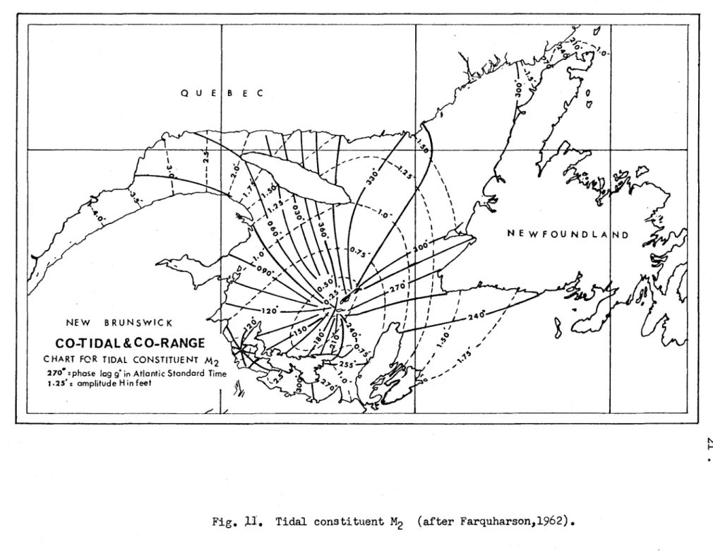
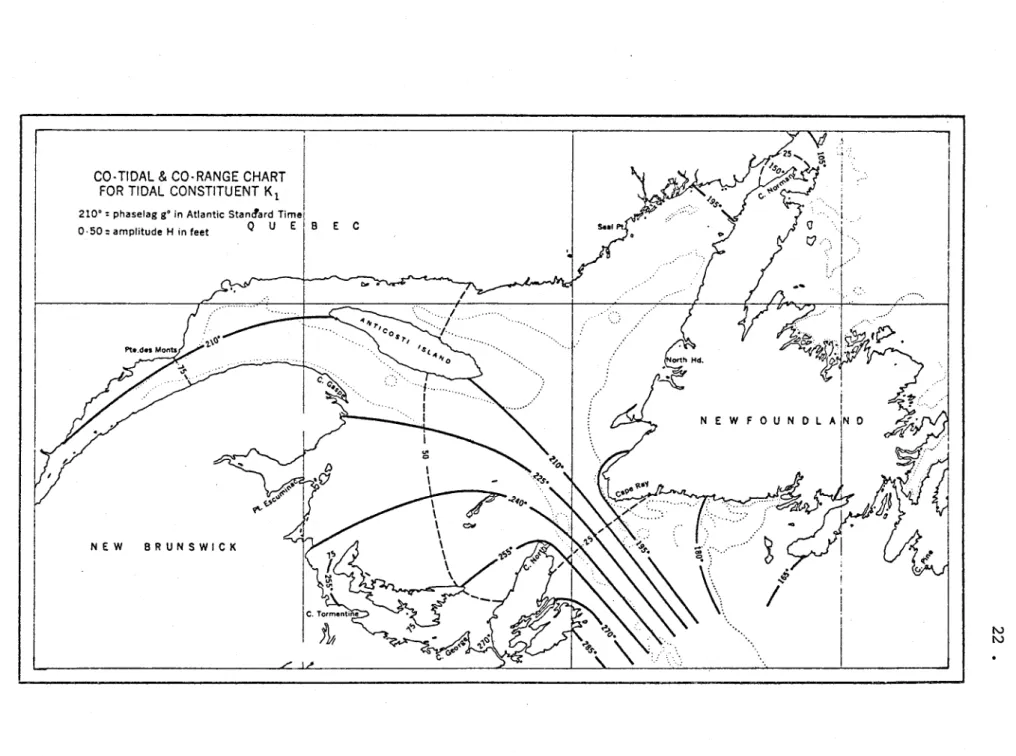
Studies of tidal phenaœna in the gulf have been reported by Dawson (1896, 1920) and Fru:quharson (1957, 1962 and 1966). The semidiurnal and diurnal tides, fran the North Atlantic Ocean, are both propagated through cabot Strait. The propagation of the tide can be rrost clearly illustrated by a cotida! chart. Figure Il shows the cotidal chart for the semidiumal Itmar tidal constituent~. It shows the influence of the Coriolis force in the reduction of the nodal line to an arrphidrœri.c point. Figure 12 shows the cotidal chart for the diurnal oonsti tuent KI.
In rrost areas of the Gulf, the semidiurnal constituent dorninates. Tidal range increases rapidly tavards the St. Lawrence River with a rœan range of about 10 ft at Father Point, 15 ft at Quebec City and l ft at Three Ri vers. The horizontal tide at Father Point has an average. peak flow of 70 million CFS, which is reduced at Quebec City to about 1.5 million CFS.
Except in the St. Lawrence Estuary, Cabot, Belle Isle and Northurrberland Straits,
am
other locall y oonfined regions, tidal currents seldan exceed 0.5 kn. In Cabot Strait, tidal streams are typically of the order of aknot. In sorre areas, the phase of the tidal stream varies significantly
with depth. Forrester (1970) suggests that the presence of an internal tide in the St. Lawrence Estuary below the Saguenay River entrance
oonsiderably influences the character of the tidal streams, particularly in the upper layer of the estuary. Internal tides probably exist
throughout the gulf, but observational evidence of their importance is still lacking. If present, their behaviour is likely to vary substantially fran season to season as the densi ty structure tmdergoes marked variation in the upper part of the water.
using the principle of continuity and water level data, Forrester (1972) was able to calculate seven harrronic constituents (~, S2' N2, KI' 01' M4
Q U E I B E C
NEW BRUNSWICK
CO-TIDAL&CO-RANGE
CHART FOR TlDAL CONSTITUENT M2
270· :phase log g' in Atlantic Standard Time
1.25': amplitude H in feet
t1
NEW FOU NOL AIN D
~
Fig.
;lI.
Tidal constituent M2 (after Farquharson,1962).N
CO-TIDAl & CO-RANGE CHART
FOR TIDAl CONSTITUENT KI
210' : phaselag g' in Atlantic Stancfard Time
0.50: amplitude H in feet Q U E B E C
NEW BRUNSWICK
NEWFOUNOL
Fig. 12. Tidal constit~ent KI (after Farqur.arson,1962).
1 ... [ .. , 1 1 }/ . ... .
23 •
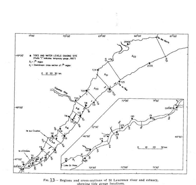
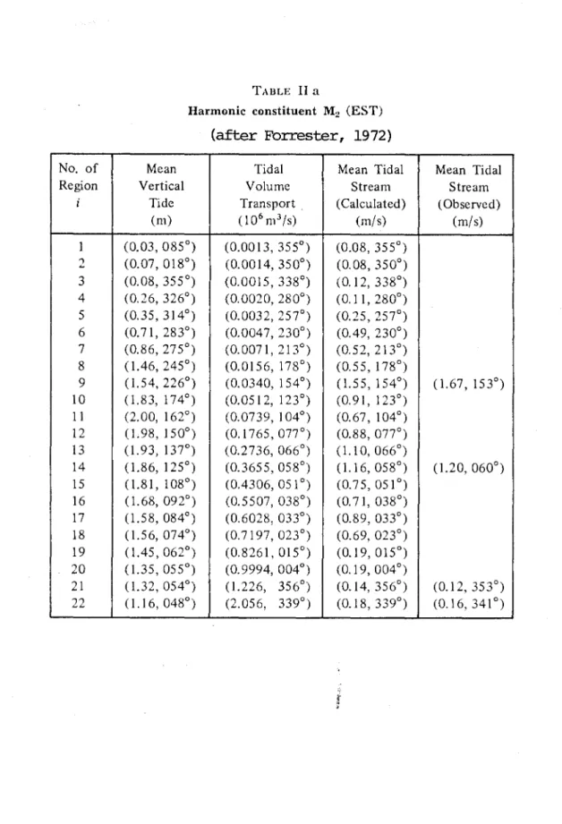
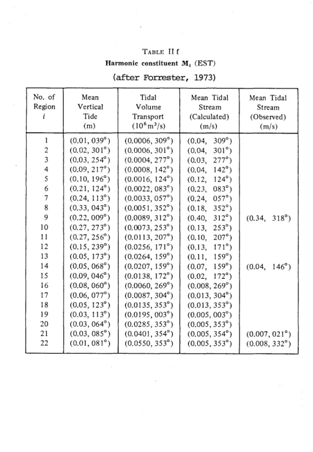
across the St. Lawrence river and esturuy (Fig. 13). Table lIa lists the ~ harrrnnic ronsti tuent of the vertical tide for each
region and of the tidal volurœ transport and rrean tidal stream through each downstream cross-section. The average ~ tidal stream through cross-sections
Ag,
1).4' ~land ~2 as obtained fram the current rreters is also shawn in Table lIa. Tables Ilb to llg contain the sarre infonnation for the harrrnnic ronstituents S2' N2, KI'°
1 , M4 and MS4 respectively. AlI phase lags refer to Este:rn Standard Tine. Inflœing tidal streams have the positive signe It was roncluded fram this study that the average tidal streams through the sections are rrore accurately detennined from the tide gauge data and the principle of continuity than rould be acconplished by direct current rreasurerœnt. This was confinned by Godin (1971), who used· a sirrple fonn of the hydrodynamic equations to study the steady and tidal flows in the St. Lawrence River and Esturuy. Tc quote fram his report: "From Trois Rivières at the rrouth of Lake St. Peter, onwards to the Gulf of· St. Lawrence the river flœ and the water level becaœ
increasingl y affected by the tide. First, the rrodifications are slight and are appreciable onl y over intervals of two weeks or rrore. Figure (14) shows the changes in level during a rronth at Trois Rivières. The daily tidal fluctuations ride on the back of a rrore irrportant
semi':"rronthly oscillation. 1bwnstream of Trois Rivières the diu:rnal and semidiu:rnal oscillations becaœ predaninant. The change in level is the shape of saw teeth when plotted on a tirre scale. The tide reaches its maxllnum arrplitude in the vicinity of the Isle aux Couldres;
downstream i t decreases and takes a more symretrical oaeanic character. Figures 15 and 16 shœ the change in level at Quebec and Pointe au Père during one nonth. Québec is a station where the tiàe has a shallow water character al though the tight tirre scale of the diagram does not
allœ to fully realize this fact, while at Pointe au Père the tide has a srrooth character.
70°00 69'00 6800d
49°00' ... TIDES AHJ WATER LEVELS GAl.IGING SITE
46°00'
(Prefix "T" indicotes lemporay gruge. 1967.) Ai' i 1h reQion.
0i " Dcrwnslrean cross-seclion of illt reQion.
o 10 20 30 km
Ile OUx Coudres
n'Yi 72'00' 71'3d FIG. 13-- Regions and cross-sections of St Lawrence river and estuary,
showing tide gauge locations.
(after Forrester, 1972;'.
24 .
25 .
TABLE II a
Harmonie constituent M2 (EST)
(after Forrester, 1972)
No. of Mean Tidal Mean Tidal Mean Tidal
Region Vertical Volume Stream Stream
i Tide Transport (Calculated) (Observed)
(m) (l06 m3/s) (mis) (mis) 1 (0.03, 085°) (0.0013,355°) (0.08, 355°) 2 (0.07,018°) (0.0014,350°) (0.08,350°) 3 (0.08,355°) (0.0015, 338°) (0.12, 338°) 4 (0.26,326°) (0.0020,280°) (0.11, 280°) 5 (0.35,314°) (0.0032,257°) (0.25,257°) 6 (0.71, 283°) (0.0047,230°) (0.49, 230°) 7 (0.86,275°) (0.0071,213°) (0.52,213°) 8 (1.46,245°) (0.0156,178°) (0.55,178°) 9 (1.54,226°) (0.0340,154°) (1.55,154°) (1.67,153°) 10 (1.83,174°) (0.0512, 123°) (0.91,123°) Il (2.00, 162°) (0.0739, 104°) (0.67, 104°) 12 (1.98,150°) (0.1765,077°) (0.88, 077°) 13 0.93, 137°) (0.2736, 066°) (1.1 0, 066°) 14 0.86, 125°) (0.3655,058°) (1.16,058°) (1.20,060°) 15 (1.81,108°) (0.4306, 051°) (0.75,051°) 16 (1.68,092°) (0.5507,038°) (0.71, 038°) 17 0.58, 084°) (0.6028, 033°) (0.89,033°) 18 (1.56,074°) (0.7197,023°) (0.69,023°) 19 (l.45,062°) (0.8261,015°) (0.19,015°) 20 (1.35,055°) (0.9994,004°) (0.19,004°) 21 (1.32, 054°) (1.226, 356°) (0.14,356°) (0.12, 353°) 22 0.16,048°) (2.056, 339°) (0.18,339°) (0.16,341°)
No. of Region i 1 2 3 4 5 6 7 8 9 10 Il 12 13 14 15 16 17 18 19 20 21 22 TABLE lIb
Harmonie constituent S2 (EST)
(after Forrester, 1972)
Mean Tidal Mean Tidal
Vertical Volume Stream
Tide Transport (Calcula ted)
(m) (l06m3/s) (mis) (0.01,112°) (0.0005, 022°) (0.03, 022°) (0.02,052°) (0.0005,018°) (0.03,018°) (0.02, 027°) (0.0005, 007°) (0.04, 007°) (0.06,003°) (0.0007,324°) (0.04,3.24°) (0.08,356°) (0.0009,304°) (0.07,304°) (0.14,329°) (0.0012,282°) (0.12, 282°) (0.18,318°) (0.0017,264°) (0.12, 264°) (0.29,294°) (0.0033, 230°) (0.12,230°) (0.34, 278°) (0.0076,205°) (0.35,205°) (0.44,221°) (0.0117,169°) (0.21,169°) (0.48,213°) (0.0177, 152°) (0.16,152°) (0.49, 197°) (0.0442, 123°) (0.22, 123°) (0.53,182°) (0.07 15, 111 0) (0.29,111°) (0.50, 162°) (0.0954, 100°) (0.30, 100°) (0.48, 142°) (O. 1117, 091 0) (0.20,091°) (0.52,129°) (0.1486,076°) (0.19,076°) (0.48, 122°) (0.1652, 070°) (0.24, 070°) (0.50, 113°) (0.2059,059°) (0.20,059°) (0.47,101°) (0.2437, 050°) (0.06,050°) (0.43, 094°) (0.3053,039°) (0.06,039°) (0.42, 095°) (0.3850, 031°) (0.04,031°) (0.34, 083°) (0.6368, 015°) (0.06,015°) 26 . Mean Tidal Stream (Observed) (mis) (0.38, 199°) (0.29, 102°) (0.03,023°) (0.06, 022°)
No. of Region i 1 2 3 4 5 6 7 8 9 10 II 12 13 14 15 16 17 18 19 20 21 22 TABLE Il c
.Harmonic constituent N2 (EST)
Cafter Forrester, 1972)
Mean Tidal Mean Tidal
Vertical Volume Stream
Tide Transport (Ca1culated)
(m) Cl 06m3/s) (mis) (0.01, 045°) (0.0003,315°) (0.02, 315°) (0.01,353°) (0.0003, 312°) (0.02, 312°) (0.02,328°) (0.0003, 302°) (0.02, 302°) (0.04,309°) (0.0005,264°) (0.03, 264°) (0.06,307°) (0.0006, 248°) (0.05, 248°) (0.10, 266°) (0.0008, 226°) (0.08,226°) (0.12, 246°) (0.0010, 205°) (0.07,205°) (0.19,225°) (0.0019, 164°) (0.07,164°) (0.33, 188°) (0.0055, 117°) (0.25, 117°) (0.28, 155°) (0.0088,094°) (0.16,094°) (0.30, 142°) (0.0124,081°) (0.11,081°) (0.36, 125°) (0.0308, 052°) (0.15,052°) (0.37,114°) (0.0497,041°) (0.20,041°) (0.33, 099°) (0.0654,033°) (0.21,033°) (0.35,082°) (0.0776,025°) (0.14, 025°) (0.30,064°) (0.0977,012°) (0.13,012°) (0.31,056°) (0.1073,007°) (0.16,007°) (0.31,049°) (0.1309, 357°) (0.13,357°) (0.30, 038°) (0.1535,348°) (0.04, 348°) (0.27,031°) (0.1887,337°) (0.04, 337°) (0.25,031°) (0.2323, 330°) (0.03, 330°) (0.24,030°) (0.4129,316°) (0.04,316°) 27 . Mean Tidal Stream (Observed) (mis) (0.30, 140°) (0.21,031°) (0.03, 330°) (0.04,318°)
No. of Region i 1 2 3 4 5 6 7 8 9 10 Il 12 13 14 15 16 17 18 19 20 21 22 TABLE II d
Harmonie constituent Kl (EST)
(after Forrester, 1972)
Mean Tidal Mean Tidal
Vertical Volume Stream
Tide Transport (Calculated)
(m) (l06m3/s) (mis) (0.02, 090°) (0.0004,000°) (0.02, 000°) (0.02, 052°) (0.0004, 35So) (0.02, 358°) (0.03,034°) (0.0004, 352°) (0.03, 352°) (0.06, 359°) (0.0005, 327°) (0.03, 327°) (0.08,353°) (0.0006, 311°) (0.05, 311 0) (0.12,330°) (0.0007,294°) (0.07, 294°) (0.14,329°) (0.0009,281°) (0.07, 281°) (0.19,302°) (0.0013, 251°) (0.05, 251°) (0.19, 288°) (0,0024, 224°) (0.11, 224°) (0.23, 263°) (0.0038, 202°) (0.07, 202°) (0.24, 253°) (0.0054, 189°) (0.05, 189°) (0.24, 246°) (0.0121,170°) (0.06, 170°) (0.23,240°) (0.0IS5,163°) (0.07, 163°) (0.25, 232°) (0.0254, 157°) (O.OS, 157°) (0.25,222°) (0.0308, 153°) (0.05, 153°) (0.24,215°) (0.0419,145°) (0.05, 145°) (0.24, 213°) (0.0471, 142°) (0.07, 142°) (0.25, 209°) (0.0596, 137°) (0.06, 137°) (0.24, 205°) (0.0721, 133°) (0.017,133°) (0.23,200°) (0.0919, 128°) (0.017,128°) (0.23,201°) (0.1157,124°) (0.014,124°) (0.23,201°) (0.2111,11So) (0.018, 118°) 28 . Mean Tidal Stream (Observed) (mis) (0.12, 227°) (0.07, 206°) (0.013, 150°) (0.015,120°)
No. of Region i 1 2 3 4 5 6 7 8 9 10 11 12 13 14 15 16 17 18 19 20 21 22 TABLE Ile
Harmonie constituent 01 (EST) (after Forrester, 1973)
Mean Tidal Mean Tidal
Vertical Volume Stream
Tide Transport (Calculated)
(m) (l06m3/s) (mis) (0.02, 052°) (0.0004, 322°) (0.02, 322°) (0.03,020°) (0.0004, 320°) (0.02, 320°) (0.03,005°) (0.0005,316°) (0.04, 316°) (0.07,336°) (0.0006, 296°) (0.03, 296°) (0.09,330°) (0.0007, 284°) (0.05, 284°) (0.13,312°) (0.0008, 271°) (0.08, 271°) (0.14, 306°) (0.0010,260°) (0.07, 260°) (0.18, 286°) (0.0014,236°) (0.05, 236°) (0.20,271°) (0.0024, 209°) (0.11, 209°) (0.22, 244°) (0.0036, 187°) (0.06, 187°) (0.24,235°) (0.0050,174°) (0.05, 174°) (0.24, 232°) (0.0113, 156°) (0.06, 156°) (0.24, 221°) (0.0172,147°) (0.07, 147°) (0.25,214°) (0.0234,141°) (0.07, 141°) (0.24, 204°) (0.0281,136°) (0.05, 136°) (0.24, 197°) (0.0381,128°) (0.05, 128°) (0.23, 195°) (0.0427, 125°) (0.06, 125°) (0.24, 192°) (0.0541,120°) (0.05, 120°) (0.23, 187°) (0.0651, 116°) (0.015, 116°) (0.22, 182°) (0.0829, 111°) (0.016,111°) (0.23, 183°) (0.1047,107°) (0.012, 107°) (0.21,183°) (0.1858,101°) (0.016,101°) 29 • Mean Tidal Stream (Observed) (mis) (0.13, 196°) (0.06, .183°) (0.010,107°) (0.015, 115°)
30 .
TABLE II f
Harmonie constituent M4 (EST)
(after Forrester, 1973)
No. of Mean Tidal Mean Tidal Mean Tidal
Region Vertical Volume Stream Stream
i Tide Transport (Ca1culated) (Observed)
(m) (l06m3/s) (mis) (mis) 1 (0.01,039°) (0.0006, 309°) (0.04, 309°) 2 (0.02,301°) (0.0006,301°) (0.04, 301°) 3 (0.03, 254°) (0.0004, 277°) (0.03, 277°) 4 (0.09,217°) (0.0008, 142°) (0.04, 142°) 5 (0.10,196°) (0.0016,124°) (0.12, 124°) 6 (0.21,124°) (0.0022, 083°) (0.23, 083°) 7 (0.24, 113°) (0.0033, 057°) (0.24, 057°) 8 (0.33, 043°) (0.0051,352°) (0.18, 352°) 9 (0.22,009°) (0.0089,312°) (0.40, 312°) (0.34, 318°) 10 (0.27,273°) (0.0073,253°) (0.13, 253°) Il (0.27,256°) (0.0113, 207°) (0.10, 207°) 12 (0.15, 239°) (0.0256, 171°) (0.13, 171°) 13 (0.05,173°) (0.0264, 159°) (0.11, 159°) 14 (0.05, 068°) (0.0207, 159°) (0.07, 159°) (0.04, 146°) 15 (0.09, 046°) (0.0138, 172°) (0.02, 172°) 16 (0.08, 060°) (0.0060, 269°) (0.008, 269°) 17 (0.06, 077°) (0.0087, 304°) (0.013,304°) 18 (0.05, 123°) (0.0135, 353°) (0.013,353°) 19 (0.03, 113°) (0.0195,003°) (0.005, 003°) 20 (0.03, 064°) (0.0285,353°) (0.005,353°) 21 (0.03,085°) (0.0401,354°) (0.005,354°) (0.007,021°) 22 (0.01,081°) (0.0550, 353°) (0.005,353°) (0.008, 332°)
No. of Region i 1 2 3 4 5 6 7 8 9 10 Il 12 13 14 15 16 17 18 19 20 21 22 TABLE II g
Harmonie constituent MS4 (EST)
(after Forrester, 1973)
Mean Tidal Mean Tidal
Vertical Volume Stream
Tide Transport (Ca1culated)
(m) (l06m3/s) (mis) (0.003, Ono) (0.0003, 342°) (0.02, 342°) (0.01, 000°) (0.0003, 336°) (0.02, 336°) (0.02, 300°) (0.0003,314°) (0.02, 314°) (0.04, 268°) (0.0004,205°) (0.02, 205°) (0.04, 251°) (0.0007,184°) (0.05, 184°) (0.07, 182°) (0.0009,148°) (0.09, 148°) (0.09, 160°) (0.0012,116°) (0.09, 116°) (0.12, 105°) (0.0019,052°) (0.07, 152e) (0.11, 073°) (0.0042, 008°) (0.19, 008°) (0.13, 324°) (0.0033,301°) (0.06, 301°) (0.13, 318°) (0.0059,260°) (0.05, 260°) (0.07, 295°) (0.0127,227°) (0.06, 227°) (0.03, 237°) (0.0139,212°) (0.06, 212°) (0.02, 109°) (0.0115,214°) (0.04, 214°) (0.04, 086°) (0.0088,230°) (0.02, 230°) (0.04, 100°) (0.0057, 284°) (0.007,284°) (0.02, 120°) (0.0055,303°) (0.008,303°) (0.02, 187°) (0.0027,344°) (0.003,344°) (0.02, 186°) (0.0034,049°) (0.001,049°) (0.0 l, 137°) (0.0056, 048°) (0.001,048°) (0.01, 162°) (0.0094,058°) (0.001,058°) (0.003, 251°) (0.0096, 089°) (0.001,089°) 31 . Mean Tidal Stream (Observed) (mis) (0.22, 349°) (0.04, 229°) (0.003,079°) (0.001,005°) .
5 10 Trois Rivières 1 15
~~'
'\)\'v~'\\J\\
20 25 October 1969Fig. 14: Dai1y Sea 1eve1 at Trois-Rivières (after Godin, 1971) 30 4.50 '" 4.00 Q) Q) ~ 3.50
Ouébec
~
!
1
~
1\ 1\ 1\~:! I~
\ \
~
!
~~~
11
\/
\
\~ ~ ~
\
~
1\
1\~
\1
,
/ \1
i~
~
l,
~
lin
Il
1j~~1 ~\I
5 10 , , , , 15 20 25 October 1969Fig·15: Dai1y sea 1eve1 at Québec (after Godin, 1971). Pointe au P~re
!
1.
I,t
!
,1,~
j!
1\:\,~I~!
iil: 1\~
il 1 liIl \
1 \ 1\~
1\ 1 1\ l, Ilïr
ïl\I~~îi
li
ï~
il
'il~~
5la
15 20 25 September 1969 1 \ \1 i 1 11
, 30q
j \ \
1\ '1\j
il
Il
1\ 1 1\l'
1 1 1 \ 1 \ \ 1 \ 1\ 1 iIl
\/1
1/
i/ \/~
\\ Il
~
i
1: \ 1 1 30Fig. 16,: Dai1y sea 1eve1 at Pte au père (after Godin, 1971). .-10.00 9.00 8.00 '" Cl:> 7.00 ~ ~ 6.00 5.00 8.00 7.00 '" Cl:> 6.00
i
5.00 4.00 w w34 •
In recent years theori tical rrodels have been used ta predict the tidal rrotion in the St. Lawrence River and EstUéUY (Godin, 1971; Karrphuis, 1969, 1970~ Partenscky and Vincent, 1965, 1968; Partenscky and Warnoes, 1969; partenscky and Ngoc Vu, 1971; Ploeg and Karrphuis, 1969). The results of these rrodels reveal that good agreerœnt can
be obtained between the predicted and observed tides wi th an accuracy of 0.1 ft for water levels and 15 minutes for ti.Iœ.
Seasonal and daily variations of sea level in the Gulf of St.Lawrence were analyzed by Seibert (1968). A correlation was found between
seasonal variations in sea level and atrrospheric pressure, leading
ta high sea levels in the early winter and low levels in the surmer. However, the response of sea level ta atrrospheric pressure was less than the pure hydrostatic relationship.
The rrean value of the water levels in the St.Lawrence Estua:ry also has a climatologica1 value (Godin, 1971). Figure 17 shows this rrean level on a monthly and yearly basis for a 10 year average at the principal stations strung along the estUéUY. The fluctuations in rrean levels decrease gradually downstream till they becaœ nearly imperceptible at Pointe au Père. At King Edward and Frontenac, there is a large drop in the level in JanUéUY and FebruaIy following the freeing of the channel fram the ice. The next feature COIITIOn ta all the curves is the increase in level in March and April created by the rrelting of the snow caver. These variations in level are :rraxim.ml
between the mouth of Lake St. Peter and Québec. Afte:rwards, the level drops unifonnly ta reach a miniIrum value in Septernber when they start increasing on accaunt of the increased precipitation.
Figures 18 and 19 show the deviation faIm the rrean yearly level of the 1l'Onthl y levels. As expected these deviations enclose each other like
28 26 24 22 20 18 16 t -w w 14 12 10 8 6 4 2
o
K l "\ \ Munthiy dr~(j :f'dr ;'y Mf'dl' t l'.t-!\ 10 Y,'ar Av!>rap' 1'J'l'J Iff,"
\
<;t l "",rellel' Hlwr Front \l
Pte auy T",\
~-"\'"
,'~
Var \v,,-~~~,_~_~
;=~~-~
Lav Ldl! ~ Sor~~
LOUIS~
T RCh'~r
Bat C la R Grond - - - . _ ..-_..---
.~----Pap > c ()Q C/l 0 co s:;. S z o < o co n 35 K E Front Pte aux T Var Ver Lav lan Sor LOUIS T R Champ Bat C la R Grond Port Que PapFigure 17: Monthly :rœan 1eve1 in the St.Lawrenœ Estuary Cafter Godin, 1971.)
36 • King Edward r - - - - . ! 6 -t---tt---Frontenac
-~~--"-T~1
1 1
-l-...
\ .•...•Monthly Deviation from the Mean Level Upper SUawrence 5+----~~-~----~----~----+_----+_----~---~----_+----_4---~ 4~···· Varennes, Vercheres , , , ... \. 3+---~~\~~----~---+----~----~---~----+-.----Lavaltrie \ Lanoraie 1-- \ \: 2 ---:..:: Ï'~ \ 1 ~ \'~ --- - - - ---.f---+---+--- ..
--f---Vi\\\ ;/ '\
Sorel \ \ . ••• r, /.... .~\ \ \ . ï \ \ \ \ .. '. ~ .... \\ l +---- ---l---\-~.-L--lè---+---+-_. ___ t-.----+---+---+---\ -\..
'.~
\\
, ... '. .... \ \.
.\ '."
/ ... ~ 3+---+---~-_4---_+----_+----+---+_--+_---+_--·-Jan Feb Mar Apr May Jun JUI Aug Sept Oct Nov Dec FIG. 18 (after <bdin, 1971).
37 •
3~~--~--~--~~--~1--~1--~1--~1--~1--~
1'. Monthly Deviation trom the Mean Level
1 \ \ Lower St.Lawrence \ ij~\ \ 2+---+---+---~~~~~----~----~----~----~----~----4_----~ 1
Jri:/~~~
/tl/.;
l ' \ ,
1
1 : ,l/,'
~\\
.. \ /... 'V
!
~I.
\ Il:: / 1 - . . ) : , Champlain ---....-/ -.- 1.·: \ Trois Rivieres ./ ---- _.: ••••••••• \ t:i Batiscan'-..-- -~... ••••••• • •••••••• ~ LU ~ --- .• ,.... ~ ~... .. •• ~ ~ Cap a la Roche ... p~.,.. . ';) .. ..,. ~. z o+---+-~~+---+---~--~~~~~----~----~----~~~~~~~~ G"~~:~:~ ~V/
~~
:::.:::.:::.::::.:::._
::::.::::.~:_.::/" ~
(:) Portneuf ~.~" ~ ~';:Y _._.-' ~. ~ ... ~t----. .. / ./ . ". ... ...::... 1 - - - -/.~./ . /'.~
"'·""'~·
... ··· .... ···k: //
2+---+---+---+---+---+---+---+---__ ~----~----~----~ 3+---+---+---+---+---~----~----~----4_----4_----_r----~ Jan Feb Mar Apr May Jun Jul Aug Sep Oct Nov Dec38 •
increasingly lessaffected by the fluctuation in the discharge. The only exception to the rule is Trois-Rivières during April which exhibi ts then larger àeviations fran rrean level than the stations on the other siàe of Lake St. Peter such as Sorel and Lavaltrie.
The rrean level rnay àeviate by as much as 1.3 rreters in Montréal
while at Québec its deviations seldom exceeds 20 centirreters. lce free conditions in Montréal should reduce the fluctuations in level appreciabl y .
39 •
1.5 TIDAL ~S:
Along the south shore of the St. Lawrence Estuary between St-Rock-des-Aulnaies and Trois-Pistoles, are a series of tidal marehes characterized by the presence of two grasses, Spartina al terniflora and Spartina patens. Man' s past and present impact on this
ecosystem and the inportance of these marshes to aquatic birds have been discussed in details by Reed and Moisan (197l). Discussing the origin of these tidal marshes the authors gi ve a concise account 'Which is guoted here: IIThe south shore of the estuary is underlain
by red, gray and green slates of Ordovician origin. In cœparison with New England tidal marshes, those of the St. Lawrence are subject to extreIœ conditions of ice, tide, current and clirnate. Furthernore there are no large bays or inlets along the south shore of the estua:ry and the shallow bays in 'Which the marshes are found offer li ttle protection fran wind, wave, current and ice action. These factors seriously affect the rate of sedirrentation (hence the build up of thick sedirrents and peat) and the expansion of existing
marshes. The St. Lawrence marshes are therefore underlain by a shallower layer of peat and sedirrent than those of New England. Another apparent particularity of the St. Lawrence marshes is their characteristically high density of small pools 'Which occur mainly near the landward border. The death of plants and the rotting of their rlllzorœs-tend te deepen
these pools. Hanelin and ca.illeux (1966), working in a small marshin the St. Lawrence Estuary, e:xplained the fonnation of pools by the action of ice and tides: blocks of turf are pulled out and transported by the ice wi th the rising tide. The larger nurrber of pools in the St. Lawrence marshes appears te be a consequence of extrerre ice and tidal action.
IIThe gradually slopping shoreline of the St. Lawrence south shore is occasionally inten:upted by high rocky outcrops. Thesaoutcrops do net
40 •
support marsh vegetation and therefore di vide the marshland into srnaller segrœnts which can be nore convenientl y described. The nost inpJrtant of these indi vidual marshes are listed and described in Table III."
l t was concluded fram this study that a large population of Black Ducks inhabi ts theSpartina marshes during the spring and surnrœr
where i t finds almost aIl of its breeding needs. Breeding populations of Cœlrron Eiders, Herring, Gulls, Great Black-backed Gulls, Great Blue Herons, Black-Crowned Night Herons and severa! species of shore birds, as weIl as migrating populations of Canada Geese, Atlantic Brant and other aquatic birds rely on this habitat as a source of food.
41 .
TAilLE I I I
Description of the tidal mar~hes of the Slllith shon: of the St. Lawrence E~tuary
--- - - - ---
---1 Icngth of* original' acreagc now* 1
Location shoreline acreage in marsh 1
__________ J __
(_n_1i_Ie_S_) _ _ ! _ _r_ac_res~
__:---(-a~~~~-_1
______________________ _ uescri ptionlaie de Ste-Anne-de-Ia-Pocatière (from Mont-des-Qurs
Il Rivière-Quelle)
4.5 1100 1 400 - S. ail. zone: relatively narrow - steep gradient - fairly deep layer of underlying sediment as il1dicated by deep drail1age channels.
1 - S. pat. zone: narr,lW with relati\'ely few RI/ppia pools.
\ - JUIiCI/S slope: narrow - prior to reclamation very wide with
Some 1
gcntle sillpe.
1
1
- SIHlrclinc marsh: cllmpktc1y climinated by agriculture. vegetation typical of thi, zone now gnl\\'Ing on dikc.
---i---I--- - - - ---
---St-Denis. to Kamouraska Kamouraska to Ste-Hélène St-André (3 miles SW ta I.S miles NE of St-André) Rivière-du-Loup (3 miles westward from Rivière-du-Loup wharf) Cacouna (1.5 miles either side of Cacouna) 3.0 1 1 6.0 1 1 ! v 1 4.:S 3.0 3.0 600 175 (also 250 reclaimcd by dike but now regene-rating into marsh - - - -940 725 -575 435 350 270 , ,- S. (III. zOl1e: as above.
- S. l'(I!. Zlll1e: biscctcd by dikc - ollhide dike narrow, considerable
1
number of RlIl'p;i/ pools - "ithin dike br,'ad \Vith few pools.
- JIIIICIiS slupe: bruad - all reclail11ed by a second dike.
1-
SIHlrcline Illar ... h: scattcrcd patches along fence rows and abanduncd fields.- S. (III. 7one: as above.
- S. l'li 1. zonc : variable ln width - high density of RI/ppin pools
-lar~e salt panne 111 this and fllllnwing zone at S\V end nf marsh.
- JIII/I'II.I· ~Inrc: f;li rly broad but IlllW almost ail reclaimed. - Shorelil1e mar~h: scattered patches along fcnce rows and araund
,
1
rocky outcrops.
- S. (III. zone: as above.
- S. plll. zone: narrnw, many pools.
- JIIIII,IS slopç: fairly broad - mainly intact except for narraw band reclaimed by dike in village. SW portion of rcclaimed land returning 10 Illarsh.
- Shorelinc Illarsh: eliminated by agricliiturai and residential developlllent.
- S. ail. zone: modcrately broad - fairly deep drainage channels.
- S. pal. zone: variable in width but generally narrow.
- JIlI/CII.I· slope : narrow but forrning a broad .. tongue .. at the mouth of the river.
- Shorclil1c marsh: mostly eliminated - heavily grazed where it
remains.
1
---700 285 - S. ail. zone: fairl)' broad on shallow sediment.
- S. {Jill. zone: modcratcly broad with Illany pools - drainage and
grazil1g ln this and the follllwing zone have led ta salI panne formation 111 central portion of marsh.
- JIIIICIIS slope : modcrately broad - only partially rec1aimed by low dikes.
- Shoreline marsh: almost entircly eliminated by agriculture.
N.il. the construction of a large sea port at Gros Cacouna (a project which ha, 110\\' bccl1 ,u,pcl1d~d shnrl of cOlllplction) ha, ,
Icd tn tllc filling il1 of <Jlmost 350 aues (ail zones) ln lhe SW pnrt!nn of this mar ... h.
* approximate measurements made from aerial photographs
1
length of
Location shoreline
(miles) Ile Verte Channel 4.31 (from above marsh
J
6.3.2.0 tn Riv.-des-Vases-also on S. shore of Ile Verte) Rivières-des-Vases 4.S to Rivière Verte original acreage (acres) 500 1200 42 . TABLuIlIcont'd) acreage now in marsh (acres) 480 1000 description
---_._--- S. lIll. zone: narrow on steep slope.
- S. plll. zone: nnrrow - comiderable salt panne formation of un-certain cause.
- JI/nel/s slope : narrow - much salt panne. some mowing on rest. - Shoreline marsh : a few small remaining tracts.
--- S. lIll. zone: moderately broad on deep to moderatcly deep sedi-ment.
- S. pl/I. zone: broad to very broad with very high density of
RI/ppi(/ pools.
- Juneus slope: variable but generally broad - about 50 acres re-claimed in E. portion of marsh - some grazing and mowing. - Shoreline marsh: one large. relatively undisturbed tract (200 fI.
by one mile) also some regencration in abanduned fields - occa-sional burning. grazing and mowing.
- - - ---1--- - - - 1 - - - -_ _ _ _ _ _ _
Rivière Verte to Pointe-à-Ia-Loupe
5.2 1800 1500 - S. ail. zone: very broad on shallow sediment.
- S. pat. zone: fairly narrow, high density of pools - in central portion draining and grazing have callsed salt panne formation.
- JrI/lCI/S slope: partially reclaimcd (one large dike encloses more th an 100 acres of this and pr('ceeding zone near SW edge of marsh). - Shoreline marsh : ail climinated exccpt a few small tracts.
43 •
1.6 IŒ:
Aerial ice sm:vey in the Gulf of St. Lawrence was first reported by
Fo:rward (1954) of the Geographical Branch of the DepartIrent of Mines and Technical Surveys, who analysed spring break-up pattenls for the 1940-1952 period. Since 1959 the Meteorological Branch of the Depart-rrent of Transport has operated an aerial ice reconnaissance in
conjunction with an iceforecasting program of the Sea lce Forecasting Central in ottawa. (For details of bibliography, the reader is referred to EI-Sabh ét al. (1969». Apart from their operational irrportance for navigation the ice charts have been and will he very useful for studies of the rœteorological effect on formation, growth, decay, and break-up of the ice in the gulf.
In the Gulf of: St. Lawrence observations show that ice corœs from three
sources; (a) Labrador ice that drifts fram arctit and subarctic areas together with small icebergs and enters the gulf through the Strait of Belle Islei (b) ice from the St. Lawrence River and Estuaryi (c) ice fields which are locally fonœd in the gulf. In general, ice starts to fonu in rnid Decerrber wi th fast ice fonning in shel tered areas i by late January alrrost the whole gulf is frozen o'iteri it reopens in late April-May. The ice charts identify four ice types in the gulf: new, young, rœdium winter, and thick winter.
Matheson (1967) has studied ice conditions over a five year period using charts published by the DepartIrent of Transport. Figure 20 shows the fortnightly average ice conditions. From these charts it can he seen that during the rronth of January the ice concentration increases rapidlYi however, the region west of Newfoundland remains
unfrozen due to the influx of water fram the Labrador current. By the last week of January and the first week of February the southwestem and central parts of the gulf are covered by heavy ice originating in
.7 Mor. 26
'11 May 21 June 4
lEGEND
D
Open water 1-3 ienths ice coyervery open pack ice
-
4-6 Tenths oce cover open pack ice-
7-9 Tenths ice cO'~erclose pack ice
-
10 Tenths ôce caver consolidated pack iceFive-year mean ice concentration (after Matheson,1967)
Fig. 20
"'"
"'"
45 •
the St. Lawrence Ri ver and Estua.:r:y. As winter progresses the ice in these areas is convected by the prevailing northwesterl y wind and current out through the southern side of cabot Strait. A typical feature seen from the charts is also the 10W' ooncentration along the north shore, which is primarily caused by the prevailing off-shore wind. A rather rapid break-up occurs over the entire gulf with the vernal wanning, leaving ice in the areas north of Prince Edward Island
and the Strai t of Belle Isle longer than in the Gaspé Passage and the central part of the gulf. Matheson' s charts are valuable for shOW'ing the geographical distribution of ice, but they do not inoorporate ei ther thickness, volurre or drift of the ice in the gulf.
Using the weekly ice summary charts, Forrester and Vandall (1968)
divided the gulfinto ten regions and estimated ice volurres and
average ice thicknesses in each of the regions at two-weekly intervals through the six ice seasons of 1962 to 1967, and also through the six year mean (1962-1967) ice season. For the mean ice seacon they found the greatest average ice thickness (24 cm) occurred in the region aIDmd Prince Edward Island early in March. OVer the gulf as a whole the
greatest average ice. thickness (16 cm) occurred at the end of February for the mean ice season.
It is essential to cany out heat budget studies in order to mderstand, and hence predict, the fonnation, grcMth, and break-up of the ice. Few complete studies of this character have been carried out in the Gulf of St. Lawrence; however, Lauzier and Graham (1958), Lauzier and Barlett
(1961), Coonbs (1962) and Matheson (1967) have investigated the subject. Matheson (1967), fran his study on the meteorological effect on ice in the Gulf of St. Lawrence, has shawn that high beat los ses during the season do not necessarily imply severe ice oonditions. As pointed out by him "computation of the heat fluxes revealed the ve:ry high heat gains or los ses which may ensue if an airflOW' type is rnaintainerlover a long