The 1st Joint International Conference on Multibody System Dynamics May 25-27, 2010, Lappeenranta, Finland
Advanced engine dynamics using MBS:
Application to twin-cylinder boxer engines
Yannick Louvigny*, Pierre Duysinx* *
LTAS – Automotive Engineering - University of Liège, B52, Chemin des Chevreuils 1, B-4000 Liège, Belgium E-mail : [email protected], [email protected]
ABSTRACT
Engine simulation is an important issue to design mechanical components and to reduce the development cost of new vehicles. Dynamic simulations of a twin-cylinder boxer engine are carried out with rigid and flexible multibody models using the finite element approach. In a first step, simulations of the engine running at constant revolution speed (4000 rpm) are done taking advantages of the actual geometry of engine parts coming from CAD models. Forces due to the gas pressure are added in the simulation to calculate more precisely the load applied on each engine part. A mixed model is developed; pistons and connecting rods are considered as rigid bodies while the crankshaft is meshed with flexible brick elements. With this model, calculation of crankshaft stresses and displacements is possible. Then, simulations are made with engine speed variations to evaluate the effect of inertia. Due to the complex shape of the crankshaft, the CPU time and computer resources can be important. As simulations with a variable rotation speed have to be carried out on a larger number of engine revolutions, it becomes difficult to work with the fully detailed crankshaft geometry. So, simplified models (a tridimensional model with simplified geometry and a beam model) of the crankshaft are developed and compared. These models are first validated with different tests including results of constant speed flexible simulations.
Keywords: Engine modeling, rigid multibody simulations, flexible multibody simulations, simplified
model, beam model.
1 INTRODUCTION 1.1 Background
Facing environmental challenges and financial crisis, automotive industry has to improve the fuel economy of new vehicles and to reduce their polluting emissions. To make cleaner car, a strategy that is widely used nowadays is the downsizing i.e. replacing large engines by smaller ones with higher specific power. In this context, small twin-cylinder engines regain interest for use in urban cars or as prime movers in hybrid electric cars. Previous works [4, 5] have pointed out the advantages and drawbacks of the boxer engine configuration (flat engine with opposed cylinders). However, for non-in-line configurations, one has not a deep understanding of their loading and their vibration behavior so that there is a need for advanced modeling and simulation tools of engine dynamics. Thus engine simulation has become an issue to decrease the emission of vibrations from the engine, to design mechanical components and to reduce the development cost of new vehicles [1].
1.2 Objectives
In this work, dynamic simulations of a twin-cylinder boxer engine are carried out with rigid and flexible multibody models using the finite element approach [2] in SAMCEF FIELD Mecano [8]. In a first step, simulations of the engine running at constant revolution speed (4000 rpm) are done taking advantages of the actual geometry of engine parts coming from CAD models. Rigid (all components are rigid) dynamic simulations are realized, with an imposed constant crankshaft rotation speed as a constraint, to calculate the inertia forces and moments in the engine. Then, the forces due to the gas pressure are added in the simulation to calculate more precisely the loads applied on each engine part. The constraint on the flywheel (prescribed rotation speed) prevents engine from accelerating or slowing down under the action
of gas pressure and so it behaves as a regulated brake torque [7]. Since, the rigid body model is not sufficient for crankshaft stresses analysis [1], a mixed model is developed (pistons and connecting rods are considered as rigid bodies while the crankshaft is meshed with flexible brick elements). With this model, calculating the crankshaft stresses and displacements is possible. Several models of crankpins and bearing surfaces (rigid hinge, rigid-flexible contact, bushing and hydrodynamic bearing) are compared [6].
In a second step, varying the revolution speed from 3800 to 4200 rpm in 0.18 seconds is considered to investigate engine unsteady states because crankshaft deformations and stresses during transient operating conditions are critical [3]. For constant speed studies, flexible simulations are carried out on two or four engine revolutions. Nevertheless, due to the complex shape of the crankshaft, the CPU time and computer resources can be important. As simulations with a variable rotation speed have to be carried out on a larger number of engine revolutions, it becomes difficult to work with the fully detailed crankshaft geometry. So, simplified models of the crankshaft are developed [10] and compared: 1/ a tridimensional model with simplified geometry (no fillet radius, no lubrication hole…) and 2/ a beam model. These models are first validated with results of constant speed flexible simulations (geometric and dynamic characteristics, strains, stresses, natural frequencies…).
2 CONSTANT SPEED SIMULATIONS 2.1 Rigid multibody model
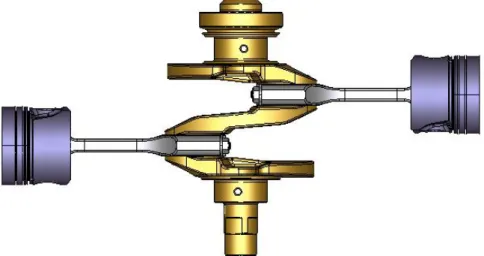
A first rigid (all components are considered as rigid bodies) simulation of the engine running at constant revolution speed (4000 rpm) is done taking advantages of the actual geometry of engine parts coming from CAD models. CAD model (in STEP format) of the two pistons, the two connecting rods and the crankshaft are imported in the SAMCEF FIELD environment (see figure 1) and the parts are linked together using appropriate kinematic joints. An imposed constant crankshaft rotation speed is used as a constraint, to calculate the inertia forces and moments in the engine. Then the forces due to the gas pressure, coming from experimental test bench, are added in the simulation. This gas pressure creates a force on the piston that is responsible for the torque of the engine. But, this force is also the source of the important stresses inside the components and it has to be simulated to determine strains and stresses of each engine parts. Since for these first simulations, we study steady states of the engine, the engine speed has to remains constant. For this purpose, a constant speed of 4000 rpm is prescribed as a kinematic constraint at the flywheel normal position.
Figure 1. Geometric model of the boxer engine in Samcef Field
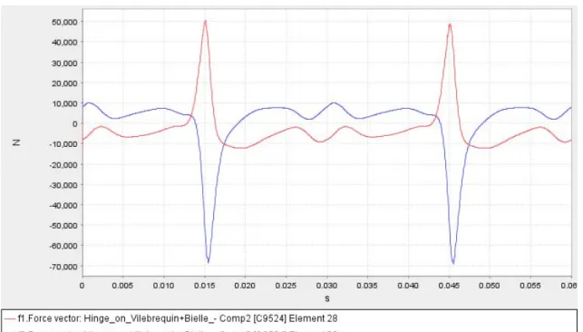
Figure 2 shows the forces that are transmitted from one connecting rod to the crankshaft during the engine operation. The radial force (red curve) reaches a maximum value of 50.000 N during the fuel combustion when the piston is 3 degrees after its top dead center (TDC). The tangential force (blue curve) is maximal at 12 degrees after the top dead center and its corresponding value is 67.500 N. The peaks of force due to
the combustion are predominant (approximately seven times the forces due to the inertia) and are thus critical for the stress and strains analysis.
Figure 2. Forces transmitted from the connecting rod to the crankshaft (4000 rpm) 2.2 Flexible multibody model
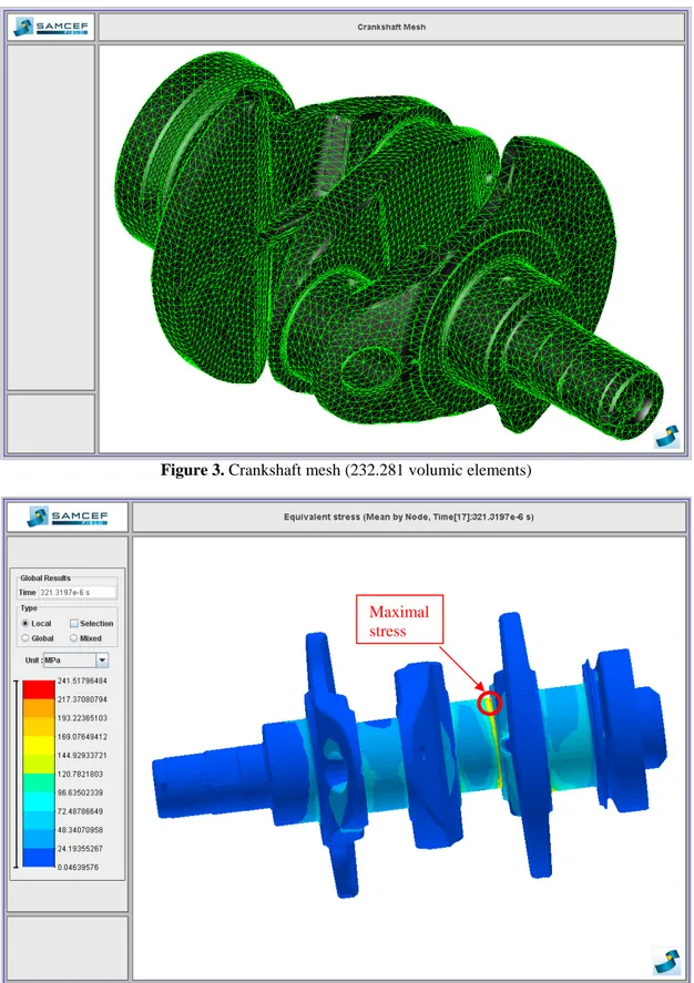
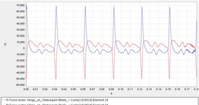
A mixed model is developed (pistons and connecting rods are considered as rigid bodies while the crankshaft is meshed with flexible elements), constraints are still the prescribed rotation speed of 4000 rpm and the pressure acting on the two pistons. With this model, calculation of stresses and displacements in the crankshaft is possible. Several models of crankpins and bearing surfaces are compared. The first simulation uses a “rigid hinge” model for the connecting rod crankshaft contacts and for the crankshaft main journals. The rigid hinge allows no translation between the two components, only a degree of freedom in rotation is permitted. The time integration algorithm used for the simulation is the Chung-Hulbert algorithm while the time step defined for results back-up is 20 µs (it corresponds to a 0,5 degree crankshaft rotation) and thus the time step for the integration process is smaller or equal to 41,67 µs. The crankshaft is meshed with linear tetrahedrons. Its complex shape imposes to use small elements so that the complete crankshaft mesh is composed of 232.281 elements (see figure 3). Using refined mesh in a multibody simulation requires a large CPU time (approximately 6 days) and computing resources. Figure 4 shows the crankshaft stresses for the bearing surfaces using a “rigid hinge” model. The maximal stress (242 Mpa) occurs at 320 µs second that corresponds to a crankshaft angular position of 8 degrees after the top dead center (this means between the radial and tangential maximal force). The maximal stress is located on the crankpin connected to the piston submitted to the maximal gas pressure. Other important stresses are located in the bearing journal next to the flywheel because all the engine torque passes through this part.
The “rigid hinge” model was the first and simplest model developed for the bearing surfaces. Other models for the connecting rod crankshaft contacts and for the crankshaft main journals were developed because these contacts appear to be a critical point of the engine dynamic simulations. One model uses a “flexible-rigid contact” that allows defining a bore diameter slightly larger to take into account a running clearance. Another model uses a “radial bushing” that is similar to the “flexible-rigid contact” but it has a radial stiffness to slow down the translational motion of the crankshaft in the bore. The radial stiffness is used to approximate the effect of an oil film. The last bearing model simulated is the “hydrodynamic bearing model” implemented in SamcefField Mecano. This model simulates the oil film behaviour by solving the Reynolds equation. A more complete description of these three models is given in [5] and [9].
In the rest of the study, the “rigid hinge” simulation is used as a reference to compare with simplified crankshaft simulations (using also “rigid hinge” models for their bearing surfaces). The “rigid hinge” model is chosen because it is well adapted to work with simplified models of crankshaft and because it gives the shortest calculation time.
Figure 3. Crankshaft mesh (232.281 volumic elements)
Maximal stress
3 VARIABLE SPEED SIMULATIONS 3.1 Rigid multibody model
In this second part, varying the revolution speed from 3800 to 4200 rpm is considered to investigate engine unsteady states. First, a rigid multibody simulation is made. This model is similar to the one of point 2.1, except that the prescribed rotation speed varies, in this case, from 3800 rpm to 4200 rpm in 0.18 seconds and the force due to the gas pressure that has been adapted to remain in phase with the crankshaft position. Figure 5 shows the forces that are transmitted from one connecting rod to the crankshaft during the operation of the engine. The radial force (red curve) reaches a maximum value of 51.000 N and the maximal tangential force (blue curve) 69.000 N. The maximal value of the forces (radial and tangential) peaks decreases at each rotation because the inertia force is increasing and is opposed to the force generated by the gas pressure when the engine speed is increasing.
Figure 5. Forces transmitted from the connecting rod to the crankshaft (3800 => 4200 rpm) 3.2 Flexible multibody model
3.2.1 Creation of simplified models
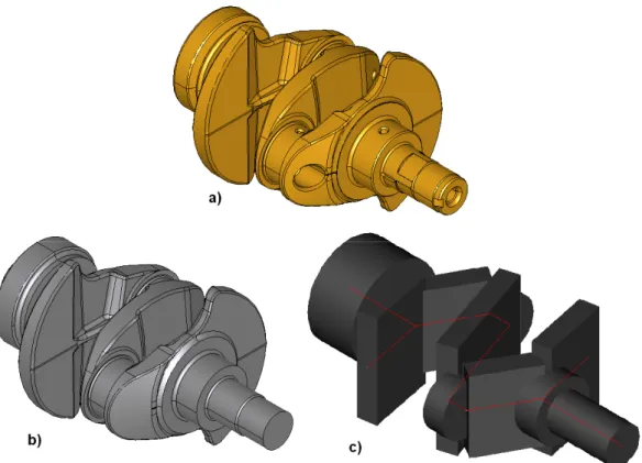
Due to the complex shape of the crankshaft, working with the actual geometry (figure 6a) in such flexible multibody simulation is impossible because the CPU time and computer resources become too high. So, simplified models of the crankshaft are developed: 1/ a tridimensional model with simplified geometry (figure 6b) and 2/ a beam model (figure 6c). Superelement models have also been considered but they are still in development.
The first simplified model is obtained by manual modification of the original CAD geometry (reduction of geometrical details). Lubrication holes, screw holes and other holes are deleted. Some fillets and chamfers are also deleted. Non- critical sections are strongly simplified. Adjacent small faces are merged to reduce the great amount of faces. After these modifications, the crankshaft can be correctly meshed with 15.569 linear tetrahedrons (a 93% decrease of the number of elements compared to the initial model). To go further in the simplification of the crankshaft, a simple beam model is designed. Crankpins, journals and both ends of the crankshaft are modelled by full circular beams of appropriate sections and crank arms and counterweights are modelled by rectangular beams.
Figure 6. Full model of the crankshaft (a), simplified 3D model (b) and beam model (c)
To evaluate the validity of these two simplified models, modal analyses are performed on them and on the fully detailed model. The five first eigenfrequencies of each crankshaft model are given in table 1. We notice that except the third values, the vibration frequencies of the simplified 3D model are higher than the ones of the complete model (approximately 10% higher). It means that the simplified 3D crankshaft is more rigid. There are two reasons; the first one is the brick elements size of the mesh (bigger elements gives a more rigid model) and the second reason is that every hole of the crankshaft is deleted and replaced by material. In the case of the beam model, the differences are more important (up to 44% for the second frequency) and the simplified model is less rigid than the complete model.
Frequency 1 Frequency 2 Frequency 3 Frequency 4 Frequency 5
Fully detailed model 746 Hz 1099 Hz 1389 Hz 1716 Hz 2057 Hz
Simplified 3D model 847 Hz 1232 Hz 1235 Hz 1851 Hz 2287 Hz
Beam model 504 Hz 690 Hz 1162 Hz 1381 Hz 1588 Hz
Table 1. Five first eigenfrequencies of the crankshaft models.
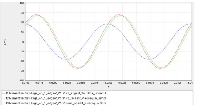
Another test is performed to evaluate the inertia and dynamic properties of the two simplified crankshaft. The 3 crankshaft models are submitted to a rotation speed (4000 rpm) and the forces and moments acting on the engine block (a ground hinge in this case) are measured (figure 7). The green curve illustrates the inertia yaw moment (around the vertical axis) generated by the original crankshaft. The blue curve corresponds to the moments of the simplified 3D crankshaft. There are two differences to note: the amplitude of the moment is smaller (45 Nm instead of 65 Nm for the maximal value) and there is a phase delay compared to the reference curve. Finally, the red curves illustrates the inertia yaw moment of the beam model of crankshaft that corresponds well to the curve of the real crankshaft.
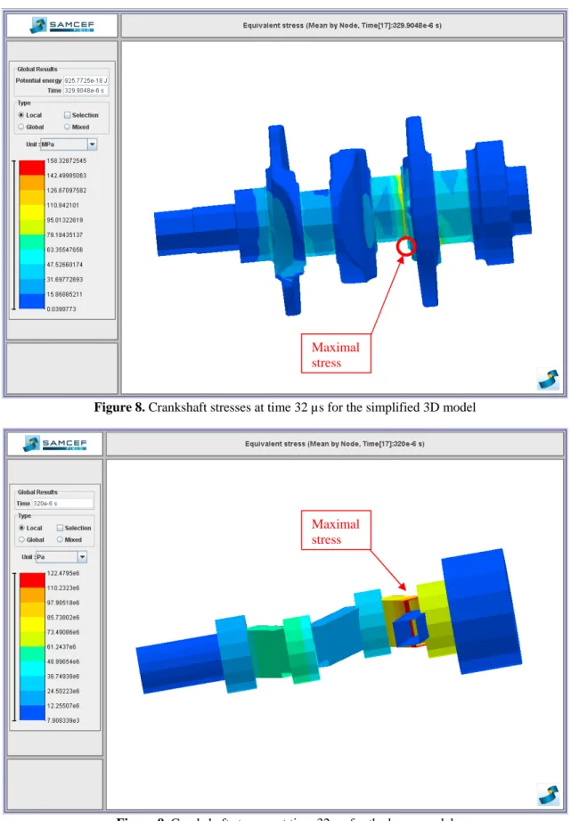
Finally, the two simplified models are tested in the mixed model developed at point 2.2. Four rotations of the crankshaft, corresponding to 2 complete engine cycles (0,06 s at 4000 rpm), are simulated for each model on the same computer (core2 duo 3 GHz CPU and 3 Gb RAM). The maximal stress measured at
time 320 µs (crankshaft angular position: 8° after TDC) is 158 MPa for the simplified 3D model (figure 8). This maximal value is quite underestimated (35 % compared to the maximal stress of the full model) nevertheless the stress localisation in the crankshaft is close to the one of the full model (figure 4). In particular, the important stresses are located on the same crankpin and on the same bearing journal. But, in this case, this value is not the overall maximum that occurs at time 720 µs (crankshaft angular position: 17° after TDC) and is 182 MPa (the maximal stress at this time in the complete model is 218 MPa). The calculation time is 15,5 hours in comparison with 6 days for the same simulation with the full model of the crankshaft. In the case of the beam model, the maximal stress measured at time 320 µs is 122 MPa (figure 9). Again, this maximal value is strongly underestimated (50 % compared to the maximal stress of the full model), but the stress localisation is correct. And the absolute stress maximum is still measured at time 720 µs as in the simplified 3D model and is 145 MPa. With this model, calculation time is only 3 minutes.
These two simplified models are not well suited to evaluate the maximal stresses. But they have proved their ability to give correct stress localisations with calculation time clearly shorter than the full model simulation. In particular, the beam model runs nearly as fast as a rigid simulation.
Maximal stress
Figure 8. Crankshaft stresses at time 32 µs for the simplified 3D model
Maximal stress
Figure 9. Crankshaft stresses at time 32 µs for the beam model
3.2.2 Simulations using simplified models
To evaluate the effect of speed variation on the crankshaft stresses, the flexible beam model is used in the simulation described at point 3.1. The main effect of the speed variation is the variation of inertia force.
When speed increases, inertia force generated by the mobile parts increases also. Since the inertia force is opposed to the gas pressure force, the total force acting on the crankshaft is reduced. So the maximal stress of the crankshaft decreases. The table 2 gives the maximal crankshaft stress at several times of the simulation, these times that always corresponds to a crankshaft angular position of 17° after the TDC.
Time (s) 0,00075 0,09295 0,15189
Speed (rpm) 3801 4007 4138
Maximal stress (MPa) 146.5 143.9 142.3
Table 2. Influence of engine speed on the crankshaft stresses
4 CONCLUSIONS
The rigid multibody simulation allows quick calculations of inertia forces and moments inside the engine. Moreover, the exact forces acting on each component are also known from this simulation but without tacking interaction of deflection and stresses. The flexible multibody dynamic simulation allows carrying out strain and stress analysis during all the engine rotation. But working with full geometric model requires a large CPU time and computing resources, so simplified models are useful to evaluate stress and determine the highly loaded areas of the engine parts with a drastic reduction of computing time. Thus, thanks to these kinds of simulation, designers can take into account stress and deformation criteria from early design stages
REFERENCES
[1] DRAB C.B., ENGL H.W., HASLINGER J.R., OFFNER G., PFAU R.U., ZULEHNER W.,
Dynamic simulation of crankshaft multibody systems. Multibody system dynamics 22 (2009), 133-144.
[2] GERADIN M., CARDONA A., Flexible multibody dynamics: a finite element approach, John Wiley, 2000.
[3] GIAKOUMIS E.G., RAKOPOULOS C.D., DIMARATOS A.M., Study of crankshaft torsional deformation under steady-state and transient operation of turbocharged diesel engines. In Proceedings of IMechE Vol. 222 Part K: Journal of multi-body dynamics.
[4] LOUVIGNY Y., Preliminary design of twin-cylinder engines (DEA thesis), Université de Liège, 2008.
[5] LOUVIGNY Y., VANOVERSCHELDE N., JANSSEN G., BREUER E., DUYSINX P.,
Dynamic analysis and preliminary design of twin-cylinder engines for clean propulsion system. In Proceedings of the multibody dynamics ECCOMAS thematic conference (Warsaw 2009). [6] MA Z.-D., PERKINS N. C., An efficient multibody dynamics model for internal combustion
engine systems. Multibody system dynamics 10 (2003), 363-391.
[7] POTENZA R., DUNNE J.F., VULLI S., RICHARDSON D., A model for simulating the
instantaneous crank kinematics and total mechanical losses in a multicylinder in-line engine. International journal of engine research Vol. 8.
[8] Samtech group, http://www.samcef.com, March 2010.
[9] VANOVERSCHELDE N., Etude de la dynamique d’un groupe motopropulseur deux cylindres à plat (Master thesis), Université de Liège, 2008.
[10] YILMAZ Y., ANLAS G., An investigation of the effect of counterweight configuration on main bearing load and crankshaft bending stress. Advances in engineering software 40 (2009), 95-104.