HAL Id: dumas-01723522
https://dumas.ccsd.cnrs.fr/dumas-01723522
Submitted on 12 Oct 2018HAL is a multi-disciplinary open access archive for the deposit and dissemination of sci-entific research documents, whether they are pub-lished or not. The documents may come from teaching and research institutions in France or abroad, or from public or private research centers.
L’archive ouverte pluridisciplinaire HAL, est destinée au dépôt et à la diffusion de documents scientifiques de niveau recherche, publiés ou non, émanant des établissements d’enseignement et de recherche français ou étrangers, des laboratoires publics ou privés.
Asymmetry of hands on modern human: a geometric
morphometric analysis of metacarpal bones
Valérie Deschênes
To cite this version:
Valérie Deschênes. Asymmetry of hands on modern human: a geometric morphometric analysis of metacarpal bones. Archaeology and Prehistory. 2017. �dumas-01723522�
Muséum national d’Histoire naturelle Universitat Rovira i Virgili
Master Erasmus Mundus en Quaternaire et Préhistoire
Mémoire de Master:
Asymmetry of hands on modern human; a geometric
morphometric analysis of metacarpal bones
Valerie Deschênes
Tuteur : Carlos Lorenzo
3
TABLE OF CONTENTS
ABSTRACTS 4
ACKNOWLEDGEMENTS 7
1. INTRODUCTION 8
Hand laterality and asymmetry 9
The aim of this master thesis: Objectives and Hypotheses 10
State of the question 12
2. MATERIAL AND METHODS 13
The individuals 13
The bones and the areas selected 14
The scanning process 17
The landmarks 19
The measures 23
The database 24
The limitations 25
Repeatability 26
Main statistical analysis 26
3. RESULTS 29
Descriptive statistics 29
Normality test 34
Two-sample paired test 38
Principal Component analysis 44
4. DISCUSSION 51 5. CONCLUSIONS 53 Results 54 Future perspectives 55 6. REFERENCES 57 LIST OF FIGURES 64
4 ABSTRACT
The subject of this master thesis concerns the asymmetry of modern human hands. The aim of this dissertation was to know which measures taken with a geometric morphometric analysis allowed us to recognize the asymmetry in metacarpal bones and to develop a method that can be reproduced in future researches.
To do so, we selected individuals from the San Pablo cemetery (13th to 15th centuries) and scanned their metacarpals with the Breuckmann surface scanner, in order to obtain a three-dimensional image of each bone. Then, we applied twenty-two preselected landmarks on every bone. Once the coordinates of the landmarks were exported in a database, we used a mathematical formula to obtain eleven measures. To study and interpret these measures, four statistical tests were made. The Two-sample paired test (T-test) allowed us to see which measures had a statistically significant difference. Our results showed that for all the metacarpals, the maximal length (ML) and the articular length (AL) exhibit the most the asymmetry between the right and the left sides, while the distal maximal breadth (DMB) follows. However, some measures don’t or almost don’t exhibit the asymmetry. Also, this test expresses that some metacarpals, like the MC1, have more measures that can exhibit the asymmetry than others, like the MC2. Finally, we did a Principal Component analysis. This test confirmed the importance of the ML and AL measures by making them the principal components in the ordination of the data. We also noticed that no individual is really different or asymmetrical, compared to the rest of the group, for all the metacarpal bones.
All these tests have allowed us to state that it is possible to discern the asymmetry in human modern hands, more specifically in metacarpal bones, using geometric morphometric analysis and this by the ML and AL measures. And that, by the results we obtained with the repeatability test and the statistical tests, we can also state that this method is effective, reliable and can be reproduce.
5 RÉSUMÉ
Le sujet de ce mémoire de master concerne l’asymétrie des mains chez l’humain moderne. Le but de cette dissertation est d’identifier quelles mesures, prises grâce à une analyse géométrique morphométrique, permettent de reconnaitre l’asymétrie des métacarpes et de développer une méthode pouvant être reproduite dans de futures recherches.
Pour ce faire, des individus du cimetière de San Pablo (13e au 15e siècles) ont été sélectionnés et leurs métacarpes ont été numérisés par l’entremise du scanner de surface Breuckmann, ce, dans le but d’obtenir une image en trois dimensions de chaque os. Ensuite, vingt-deux points d’intérêts (landmarks) ont été apposés sur chacun des os. Une fois les coordonnées des points exportées dans une base de données, une formule mathématique fut utilisée afin d’obtenir onze mesures.
Afin d’étudier et d’interpréter ces mesures, quatre tests statistiques ont été réalisés. Le test apparié à deux échantillons (T-test) a permis d’observer quelles mesures ont une différence significative statistiquement. Nos résultats démontrent que, pour tous les métacarpes, la longueur maximale (ML) et la longueur articulaire (AL) expriment le plus l’asymétrie entre les côtés droit et gauche, suivi par la largeur maximale distale (DMB). Cependant, certaines mesures n’expriment pas ou presque pas l’asymétrie. Également, ce test démontre que certains métacarpes, comme MC1, ont plus de mesures pouvant exprimer l’asymétrie, que d’autres, tel MC2. Finalement, une analyse des Composants Principaux a été faite. Ce test a confirmé l’importance des mesures ML et AL en faisant d’elles les composantes principales dans l’ordination des données. Il a aussi été noté qu’aucun individu est réellement différent ou asymétrique, comparé au reste du groupe, et ce pour tous les métacarpes.
Tous ces tests permettent de déclarer qu’il est possible de discerner l’asymétrie des mains chez l’humain moderne, grâce à une analyse géométrique morphométrique et ce par les mesures ML et AL. Et que, par les résultats obtenus avec le test de répétabilité et les tests statistiques, il est aussi possible de déclarer que cette méthode est efficace, valide et peut être reproduite.
6 RESUMEN
La presente memoria estudia la variación de la asimetría de las manos en los humanos modernos. El objetivo principal del trabajo es identificar cuáles medidas, de acuerdo al análisis geométrico morfométrico, permiten reconocer la asimetría de los metacarpos. Así, se busca desarrollar un método que pueda ser reproducido en futuras investigaciones.
Para esto, se han utilizado los metacarpos de los individuos del cementerio de San Pablo (siglos XIII al XV), los cuales han sido digitalizados a través del escáner de superficie Breuckmann. De esta manera, se obtuvo un modelo en tres dimensiones de cada uno de los huesos. Posteriormente, se situaron veintidós landmarks tridimensionales sobre la superficie, cuyas coordenadas se utilizaron para obtener once variables de cada uno de los metacarpos.
Para poder estudiarlos e interpretarlos, se aplicaron cuatro pruebas. El test para dos muestras pareadas (T-test) permitió la identificación de cuatro medidas con una diferencia estadística significativa. Nuestros resultados demuestran que, para los metacarpos, son la longitud máxima (ML) y la longitud articular (AL) que presentan el mayor grado de asimetría entre los lados derecho e izquierdo, seguido por la máxima anchura distal (DMB). En cambio, otras medidas apenas presentan asimetría. Así también, este test da cuenta de que, ciertos metacarpos, como el MC1, presentan más medidas que puedan explicar la asimetría que otras, como ocurre con MC2. Finalmente, se efectuó un análisis de componentes principales que confirmó la importancia de las medidas ML y AL, haciendo de ellas elementos centrales en la ordenación de los datos. Por otra parte, se observó que ningún individuo es realmente diferente o asimétrico comparado con el resto del grupo.
Todas estas pruebas nos permiten afirmar que es posible distinguir la asimetría de las manos en los humanos modernos gracias al análisis geométrico morfométrico, específicamente mediante las medidas ML y AL. Sumado a esto, los resultados obtenidos del test de repetitividad y las pruebas estadísticas, sugieren que este método es eficaz, válido y reproducible en otros casos.
7 ACKNOWLEDGEMENTS
The realisation of this master thesis would not have been possible without the support of some people and institutions.
I would like to thank my supervisor; Carlos Lorenzo Merino, for explaining to me everything I needed to know. You were always kind and clear and you always did your best to be sure that I understand, whatever it was in English, French or Spanish. I would like to thank all the people in the Institut de Paléontologie Humaine of the Muséum national d’Histoire naturelle for their support along these two years; and specially Chafika Falguères for answering all my questions and demands, as crazy as they were sometimes. Thanks to the MNHN for letting me go all around the world and have the maximum experience of the Quaternary and Prehistory master.
I would like to thank the people at IPHES and URV for letting me use the laboratory and the different facilities. I met kind and helpful people in these places. Thanks to the people in charge of the San Pablo collection for letting me use it.
I would like to thank my international friends. Whatever it was in Paris, in Tarragona, in London, in Maçao, in Nanjing or in Manila, you made this experience great. Thanks to all the flatmates I had, for understanding that I was unsocial and stressed. A special thanks to Justine Dumesnil. And a great thanks to Eduy Urbina and Sandra Rebolledo for the “physical” help regarding the writing of this thesis.
I can’t forget all my family and friends at home. Merci de m’avoir enduré, de près ou de loin, d’avoir toujours été là pour moi, peu importe où je suis et où j’en suis.
Finally, none of that would have been possible without the financial support I received. Thanks to the Aide financière aux études of the Ministère de l’Éducation et de l’Enseignement supérieur du Gouvernement du Québec (Canada). Thanks to the Erasmus Mundus program, to the Museum national d’Histoire naturelle and to the Sorbonne Université for the mobility and transportation scholarships.
8 1. INTRODUCTION
The human hand is particular. It allows us, among other things, to be precise and to grab things easily. We use our hands as tools. But, because we use one side more than the other, even if they look alike, our two hands are not exactly the same. They are asymmetrical and it is created by handedness or laterality, which is mostly unique for each individual.
This present dissertation is the reflection of the work of a master thesis studying the asymmetry of hands, more specifically of the metacarpal bones of modern Homo sapiens by a geometric morphometric analysis. The general objective of the master thesis is the work and study of a new methodology. Over this dissertation, we will explain how this methodology is important and the processes that brought our results. The current chapter will serve to put in context the present research; we will detail the general aspect of our subject. The aim of the master thesis, the objectives and the hypotheses will also be revealed in this part.
In the following chapters of this dissertation we will describe and explain our processes of how we were able to answer our questions.
The next chapter (chapter two) concern the material and methods used. We will describe our assemblage, where it came from and why it was appropriate for our research. We will also explain why the choice of the metacarpals was made and which parts of it were studied. Finally, we will describe the tools used and how we used them to collect the data we needed for the statistical analysis.
The third chapter concern the results. We will demonstrate the different outcomes of the many statistical tests we applied, more specifically for the Two-sample paired test (T-test) and how the results are important in order to answer our questions.
In the fourth chapter, we will explain our interpretations of the data according to the results of the different statistical tests and what it can mean. This chapter is dedicated to the discussion.
The fifth chapter is devoted to the conclusions. In this part, we will summarize our results and interpretations and, mostly we will answer our questions.
The chapters six is constituted of the references, and a list of the figures used in this dissertation is at the end.
9 Hand laterality and asymmetry
As we get older, our bones evolve and change. Bones carry the markers of our life. Markers are created by the activities that we do. The traces left by the muscles and ligaments are called stressed markers (White et al. 2012). The markers can be studied and can give us answers about many questions we have concerning humans; locomotion, ontogenesis, cognition and evolution (Cartmill et al. 2012, Heyes 2012, Hopkins et al. 1993, Liu et al. 2009, Steele & Mays 1995, Ward et al. 2014). To analyse the markers of the bones, different methods are used; like X-rays, manual measurements by calliper, cortical analysis and geometric morphometric analysis. One of the markers we can observe concern the differences between the bones, it is the asymmetry as an expression of the hand laterality.
Hand laterality is linked with cognition, language, the ability to make tools and much more (Corballis 1989). It is important to study hands in order to understand better how the brain works, and by that to understand better the human evolution and Homo sapiens itself.
For many years now, we know that the hand laterality is important for Homo sapiens and all the hominines (Corballis 1989). Hand laterality is the fact that most of people have a “preference” for using their left or right side, in most activities they are doing. It is in fact that we use preferably one hemisphere of our brain. We can see on the bones the marks of the laterality, it is the asymmetry, the differences in size and shape between the left and the right sides. The asymmetry is developed by the use of one side of the body more than the other during the life of an individual. Both sides, left and right, developed markers that are slightly different, resulting in an asymmetry. Two main types of asymmetry exist; fluctuating and directional. Fluctuating asymmetry is the variation between the left and right sides created by a stress. In fluctuating asymmetry, there is usually an external factor that influences the development and makes it not equal for both sides (Bonzom 1999). It refers to non-symmetry due to genetic or environmental pressures experienced through the development of an individual.
10 The directional asymmetry is not a variation across the population. It is the fact that one side, the same for every individual, is bigger than the other. There is no influence from an external factor, by a stress (Van Valen 1962).
Over the years, researches have observed the asymmetry in the human body and in other living beings (Albert & Greene 1999, Blackburn & Knüsel 2006, Corballis 1983, Corballis 1989, Hopkins et al. 1993, Hopkins et al. 2007, Kivell et al. 2011, Liu et al. 2009, Mays et al. 1999, Reuter-Lorenz & Miller 1998, Schaafsma et al. 2009, Service 1999, Steele & Mays 1995, Volpato 2012). We can clearly state that there is asymmetry in different skeletal parts. Researches also have been made to observe more specifically the asymmetry of hand related to laterality in Homo sapiens (Livshits et al. 1998, Plato et al. 1980). These studies attest that there are differences between the left and the right hand bones of the same individual; we can see the asymmetry of the hands. By knowing how to recognize and how to measure the asymmetry of hands, we have the ability to determine the laterality of individuals and to go on with more studies about brain development, cognition, evolution, language, tools making and more.
The aim of the present thesis: Objectives and Hypotheses
The purpose of this master thesis is within the physical anthropology framework. It was intentionally chosen that all the individuals studied were Homo sapiens because, it is by knowing the marks of laterality left on modern human bones that we will be able, eventually, to apply this method of analysis on fossils of hominines or other hominoids.
The aim of the present thesis is to understand which measurements, taken by geometric morphometric analysis, allow us to recognize the asymmetry in metacarpal bones related to the laterality of an individual, and the relevance of using this type of analysis. We also want to develop a method that can be reproduced in future researches.
11 Our general objectives are:
1) To analyse the metacarpal bones of Homo sapiens individuals in order to see signs of asymmetry that are associate with handedness lateralisation,
2) To do a morphometric analysis in 3D of the diaphysis, the epiphysis and of the articular surfaces of the metacarpal bones.
Our specifics objectives are:
1) To scan the metacarpal bones in order to obtain three-dimensional models, 2) To apply the preselected landmarks on the three-dimensional models of each
metacarpals, and to export the coordinates of the landmarks in a database, 3) To calculate the measures, with the three-dimensional coordinates and the
mathematical formula,
4) To do a statistical analysis of the data in order to understand better the data and to answer the questions,
5) To interpret the results of the statistical analysis in order to determine which measures exhibit better the asymmetry.
Our hypotheses are:
1) That it is possible to discern the asymmetry by measurements of the metacarpal bones using geometric morphometric analysis (3D),
2) That the measures that will exhibit better where the asymmetry is more manifested are the ones from the articular surfaces (proximal and distal).
12 State of the question
Over the years, hand laterality and asymmetry were studied by many anthropologists. Papers have been published in the past about this subject. However, no 3D morphometric analysis has been done on this matter. However, a good revue of literature was important. Some authors developed methods, measurements and statistical analyses that were relevant for the realisation of this dissertation.
Mays et al. (1999) talk about the lateral asymmetry by studying, morphologically, clavicles from a medieval assemblage, in pair. They are using statistical tests, like the Two-sample paired test, that are relevant for our research.
The statistics used by Plato et al. (1980) are also useful in our case. The latter are studying the bilateral differences in hand and cortical bones. Their research gave us also useful information about measurements of metacarpals.
In their 1998 publication, Livshits et al. explain the measurements they took relatively to study hand asymmetry. In their publication, they used radiographs to study fluctuating asymmetry and coefficient of variation in hand bones.
Vandermeersch & Trinkaus (1995) give measurements they took on a Neanderthal hominine. They did measurements on clavicles, humeri, radii and ulnae for both the left and the right sides in order to describe and compare them with other specimens. Albert & Greene (1999), Blackburn & Knüsel (2006) and Steele & Mays (1995) did different studies on bilateral asymmetry in postcranial bones. They compared asymmetry of the right and the left sides but also included different variables like sex and age.
General knowledge of human laterality and the concept of asymmetry are primordial for the well understanding of the subject of this thesis, Corballis’ publications (1983, 1989) were of a great help. He explained the origin of the laterality in human in comparison with other primates, and the link of laterality with cognition, tool making, language and more.
Slice (2007) and Zelditch et al. (2012) along with Weber & Bookstein (2011) and Zollikofer & Ponce de Leon (2005) published articles and books about geometric morphology and about the work with virtual images. To work with three-dimensional
13 models requires different instruments and methods than to work with the physical bones. Their publications are useful as guides about this way of research.
Buikstra & Ubelaker (1994) developed methods to analyse data collection of human bones. They explained the growth patterns and how to identify the sex and age of an individual. These methods were used to have information about the individuals used for this research.
A revue of literature gives information about what was made in the past and what can be applied in this study. It is a new methodology but the general concept of the determination of the asymmetry regarding the handedness or laterality is not new and gave results that cannot be ignored.
2. MATERIAL AND METHODS The individuals
This research was done with the help of a collection of fifty (50) individuals that are coming from individual graves from the medieval cemetery of San Pablo (Burgos) in Spain. The individuals are dated between the 13th and 15th centuries.
All our individuals are Homo sapiens. These individuals, twenty-five (25) males and twenty-five (25) females, have been chosen because of the good conservation of the bones, as well as for the complete information obtained from them (sex, biological age and pathologies). All the individuals are adults to prevent any bias that a still growing and changing individual, such as a child or teenager, can represent (Buikstra & Ubelaker 1994, White et al. 2012). Our individuals have a biological age between 18 and over 50 years old.
The sexes and biological ages were previously identified by a team, using mostly Buikstra & Ubelaker (1994) methods.
Well-preserved individuals in anatomical connexion, along with their information are essential for the good proceedings of this research. That ensures the reliability of the results by reducing extrapolation of the data.
14 The bones and the areas selected
The human hand is composed of nineteen bones (Figure 1). The five metacarpals are the most proximal bones. The five proximal phalanges are the first bones of the fingers. There are only four intermediate phalanges; the thumb is lacking this bone. Finally, the five distal phalanges are the bones at the end of the fingers. The hand bones are long bones aligned in rays (fingers). The rays of the hand are numbered from one (the thumb) to five (the little finger) (White & Folkens 2005).
The bones have articular surface at their proximal and distal ends for the articulation with the other bones. Metacarpals articulate with the carpal bones (bones of the wrist) at the proximal end and the proximal phalanges at the distal end. Proximal phalanges articulate with the metacarpals at the proximal end and intermediate phalanges at the distal end (except for the thumb which has his proximal phalange articulated with the distal phalange). The intermediate phalanges articulate with the proximal phalanges at the proximal end and the distal phalanges at the distal end. And, the distal phalanges articulate with the intermediate phalanges at the proximal end (except for the thumb which has his distal phalanges articulated with his proximal phalange).
The human hand is considerably mobile and has adroitness. To have this ability, the hand possesses, in addition to the bones, a great number of muscles and ligaments (Patzer 2007). These muscles and ligaments leave traces that we can see on the surface of all bones of the hand (markers) and can shape the bones differently not only for each bone but for each individual.
15
Figure 1. Right hand, dorsal. Image from White & Folkens 2005
The metacarpal bones (MC) are bigger than the phalanges. Their head (distal end) is rounded and covered by the articular surface; it is quite similar for all of the metacarpals, while the base (proximal end) is mostly rectangular. The general shape of the diaphysis is tubular with a palmar face slightly concave and the dorsal face slightly convex. They are going from bigger to smaller starting from the second metacarpal to the fifth metacarpal. All the metacarpals have different shapes (Figures 2 and 3). The first metacarpal (MC1) has a general shape larger and shorter with a robust diaphysis; it also has a saddle-shaped proximal articular surface. The second metacarpal (MC2) has a long diaphysis. Its articular surface of the base has a notch, for the articulation with three carpal bones (trapezoid, capitate and trapezium), while it has also an articular surface on its medial side for the articulation with the third metacarpal. The third metacarpal is characteristic for its styloid process at is proximal end, which is latero-dorsal. It has a proximal articular surface for the articulation with one carpal bone (capitate), a lateral articular surface for the articulation with the second metacarpal and two medial articular surfaces for the articulation with the fourth metacarpal. The general shape of the proximal base of the fourth metacarpal bone (MC4) is squared with a half-moon form on its middle. It articulates on its proximal end with carpal bones (capitate and hamate); on its lateral side of the proximal end with the fourth metacarpal (two articular surfaces) and on its medial side of the proximal end with the fifth metacarpal. The last but not least is the fifth
16 metacarpal (MC5). It is the smallest of the metacarpal bones. It possesses one articular surface on its medial side of the proximal end with the fourth metacarpal and no articular surface on its lateral side considering that it is the last bone. Although, it has another articular surface on its proximal end that correspond to the articulation with one carpal bone (hamate) (Platzer 2007, White & Folkens 2005, White et al. 2012).
Figure 2. Metacarpals from the right hand, dorsal. From MC1 (left) to MC5 (right). Image from White & Folkens 2005
Figure 3. Metacarpals from the right hand, palmar. From MC5 (left) to MC1 (right). Image from White & Folkens 2005
17 For this master thesis, we decided to analyse only the metacarpal bones. In the hand, the metacarpals are the bones that received most of the pressure. So, they are the bones that can exhibit the most the asymmetry due to handedness. All five metacarpals of the hand were analysed. This choice over others, like the study of specific fingers or the inclusion of the phalanges and of the surface areas, was made due to time limitation for the realization of this master thesis and due to the fact that not all individuals preserved all of their hand bones by pair (right and left). Our priority was the analysis of the metacarpal bones in the purpose of developing a good methodology. Also, few researches focus on only metacarpals, most of them focus on specific rays (fingers) or different bones. Consequently, we decided to take measures from different places on the diaphysis, the epiphysis and on the articular surfaces; therefore most of the bone is included in the analysis.
From our collection of fifty (50) individuals, forty (40) individuals were selected, twenty-one (21) males and nineteen (19) females. These individuals were chosen mainly because they have all of their metacarpal bones represented by the pair (right and left), which is essential for the comparison intra individual. This number of individuals allows us to remove some of the bones or measurements if they are not appropriate (broken bone, pathology, etc.), and still have enough individuals remain to have a sample of an appropriate size (around thirty (30) individuals) for the quality of the statistical analysis.
Although we know the sex of the individuals, we did not use this information to segregate more the data. In our case, the sex is not requisite. In different studies, Albert & Greene (1999), Blackburn & Knüsel (2006) and Steele & Mays (1995) showed that there is no particular difference, statistically, in the asymmetry of bones, between males and females.
The scanning process
The first step was to scan the bones with the 3D scanner Breuckmann. The scanning process consists of obtaining three-dimensional models of the metacarpal bones. The resulting images were then used for the analysis.
18 The majority of the right hands were scanned by Fotios Alexandros Karakostis for his master thesis in 2015 (Karakostis 2015). It was necessary to scan the metacarpals of the left hands as well as a part of the right hands that had not been made previously. At the same moment, the 3D images of the bones were treated by the software Geomagic (mesh doctor).
The scanner that we used was a Breuckmann SmartScan (Figure 4) with the software OPTOCAT 2012 and an automatic turntable platform. This scanner is a surface scanner. It works with three digital cameras and sends a light that reflects on the scanned object. By capturing the reflection, the scanner is able to record the spatial depth, the distance between the object and the cameras. It will then create an image with the different points captured and by combining them together (Figure 5). Photographs can be taken at the same time to record the texture and the color. That will result in a three-dimensional model of the object (Zollikofer & Ponce de Leon, 2005).
Figure 4. Scanner Breuckmann Smartscan Image from http://www.smartscan3d.co.uk/
(July 26, 2017)
19 In order to have a high-resolution image, lens of M-250 were used. We scanned over five hundred (500) bones; including the phalanges that were not included in the final work for this master; with texture, color and geometry. All of the adjustments were the same for each of these bones. The scan was set to Automatic, the parameters were set to full-resolution, with a number of captures of four, with seven scans per rotation. The Teach option allowed us to set the lights and cameras of the scanner at the appropriate distance from the bone. We placed the bones in a vertical position on the turntable platform. The Scan option obtained for us the images of the scanned bone. After alignment of the images and their merging, the 3D data result was exported in a .ply format. These .ply files were then imported in the Geomagic Studio 2013 software and were treated with the Mesh Doctor option.
The scanning process took place in the laboratory of Paleoanthropology at the Catalan Institute of Human Paleoecology and Social Evolution (IPHES).
The landmarks
Once all the bones were scanned, it was time to decide which landmarks will be use. The landmarks are points, dots that are applied on the three-dimensional image of the bone. The landmarks can then be exported in raw data that will give coordinates (x, y, z) (Zelditch et al. 2012). These coordinates will be saved in a general database.
The main benefits of the new technology are the precision in the taking of the measures as well as the possibility to have more of these measures. In the prior researches, measures were taken manually, with callipers on X-rays or directly on the bones. These methods are valid but a three-dimensional image gave us more precision in the application of the points because we can manipulate the image more easily and increase the image to be closer to the bone (zoom) as for a better visibility of the entire bone. Also, using a 3D model, instead of the physical bone, guaranties less manipulation of the bones, so a better preservation of it, which can be precious in fossils cases or damaged bones.
Because it is the first time a geometric morphometric analysis study is made about this subject, we had to make a decision and choose the appropriate landmarks that will
20 help answer our questions. The landmarks were chosen in regard of the literature and researches, and about the measures that they published.
For the sake of this dissertation, we used mainly landmarks that were coming from classical measurements, from a semi-standardized system. Most of the time these measures are taken following the works inspired by Martin (1928) and Martin & Saller (1957) who developed a great methodology for anthropologists. Case et al. (2015), Franks & Cabo (2014), Livshits et al. (1998), Plato et al. (1980), Vandermeersch & Trinkaus (1995) are some authors that used different measurements, on hand bones or other long bones from the upper limb. We selected our measurements according to what they published. The landmarks were then created from the measures we wanted to obtain. More landmarks could be added to have more measures, however due to time restriction we decided to use only the measurements that were used in previous analyses. Also, this allows us to compare the different methods and to see if the geometric morphometric analysis is useful in this kind of research.
After a period of experimentation, a conclusion of landmarks and the exact places where to place them was reach (Table 1 and Figure 6). We applied twenty-two (22) landmarks on each metacarpal of our forty (40) individuals with an objective of having all the points at the same place for all the bones. The landmarks that go together (rightmost/leftmost, palmar/dorsal) are in a straight line that is perpendicular to their opposite measure (rightmost-leftmost/palmar-dorsal). Each landmark was export in raw numerical data; in three-dimensional coordinates (x, y and z), and put in a database.
21
Landmark Definition
1 Most proximal point of the base 2 Most distal point of the head 3 Centre of the proximal articulation 4 Centre of the distal articulation
5 Rightmost point of the proximal epiphysis 6 Leftmost point of the proximal epiphysis 7 Most dorsal point of the proximal epiphysis 8 Most palmar point of the proximal epiphysis 9 Rightmost point of the proximal articulation 10 Leftmost point of the proximal articulation 11 Most dorsal point of the proximal articulation 12 Most palmar point of the proximal articulation 13 Rightmost point of the midshaft of the diaphysis 14 Leftmost point of the midshaft of the diaphysis 15 Most dorsal point of the midshaft of the diaphysis 16 Most palmar point of the midshaft of the diaphysis 17 Rightmost point of the distal epiphysis
18 Leftmost point of the distal epiphysis 19 Rightmost point of the distal articulation 20 Leftmost point of the distal articulation 21 Most palmar point of the distal articulation 22 Most dorsal point of the distal articulation
22
Figure 6. Landmarks applied on left MC2 of SP133, from proximal view, dorsal view and distal view. The numbers correspond to the numbers in Table 1.
23 In order to apply the landmarks the software Landmark version 3.0, from the Institute for Data Analysis and Visualization (IDAV) was used. The software allows us to create a new project and to import a .ply file that give access to the three-dimensional image of the bone. Once we have the image of one of the metacarpals, it is possible to move it in every positions needed. By selecting the add single point option, we were able to place the landmarks at the preselected positions. Once all the landmarks were correctly positioned, we exported the data in Raw Landmark Points (.pts). We were then able to import the three-dimensional coordinates x, y, z of each landmark via the .pts files in an Excel database.
The measures
The landmarks are going in pairs that allow us to have eleven measures (Table 2). These measures are the important data of this work. We used them to do the statistical analysis and the comparison between right and left metacarpals. Once all the landmarks were exported in the database from their .pts files, we used a mathematical formula to obtain the measurements, in millimeters. To confirm the accuracy of the formula, we also did manual measurements with a digital calliper on an individual (SP26). All the measurements were conclusive.
The mathematical formula is the following:
24
Landmarks Definition of the measure Abbreviation
1-2 Maximum length ML
3-4 Articular length AL
5-6 Proximal maximal breadth PMB
7-8 Proximal maximal height PMH
9-10 Proximal articular breadth PAB
11-12 Proximal articular height PAH
13-14 Midshaft breadth MB
15-16 Midshaft height MH
17-18 Distal maximal breadth DMB
19-20 Distal articular breadth DAB
21-22 Distal articular height DAH
Table 2. Description of the measures obtained with the coordinates of the landmarks and the formula, and their abbreviations.
The database
The database we created for the compilation of all our data was made from an Excel sheet. In the first column we have our individuals in order of number (SP5, SP8, SP10, etc.); each individual is there ten times, once for each of the five metacarpals of the two hands. In the second column, we have the sex (F for female, M for male) of each individual. The third column is for the bones, from MC1 to MC5, twice for each individual to correspond with the two hands. The fourth column was used to indicate the side (R for right and L for left) of each bone. From the fifth column to the seventieth column, the data is separate following the twenty-two (22) landmarks and their three coordinates (x, y, z) (Table 3). The final eleven columns are for the results of the measures obtained with the formula from the landmark’s coordinates. Finally, some blue color was used to segregate the data, the color was applied when the coordinates were false or incomplete – like for a broken bone. We applied the color to the coordinates and to the corresponding measure. This was to avoid errors and to avoid collecting non representative data.
25 From that database, others were created; one for each metacarpal without the landmark’s coordinates, and one for each metacarpal without the landmark’s coordinates and with the side as a separation of the measures instead of separation of the individual (Table 4). The advantage of having many databases containing the same data differently is that it is easier to use it, depending on the statistical tests or other analyses we wanted to do.
Table 3. Example of the database. Expression of the data from the fifth to the seventieth columns, corresponding to the coordinates of the landmarks.
Table 4. Example of a database. Expression of the data using the side as a separation of the measures, per metacarpal.
Limitations
The positioning of the points comported certain limitations. Some were the consequences of the lack of experience from the student, others were resulting from the software itself, and finally a few are coming from the bones themselves. The most important limits noticed were the exactness in the position of the points, especially when the bone was twisting or for the midshafts measurements, the non-possibility to do undo and the poor visibility of the bone in certain position. The transfer of the data was also a possible place for error by the fact that it needed a lot of manipulation of the data. Plus, we also noticed that with a higher resolution image, it was not more easy or precise to position the points, but it would slow down the process considerably.
Landmark 1 Landmark 2
L1-X L1-Y L1-Z L2-X L2-Y L2-Z
-3,12E+07 1,43E+08 9,41E+07 -5,82E+07 1,23E+08 5,15E+08
4,27E+07 -2,45E+06 6,46E+08 3,29E+07 -6,48E+07 8,68E+05
Mesures
ML - R ML - L AL - R AL - L
26 After a period of tests and experimentations, despite the limitations; errors and inaccuracies were resolved and avoided, and we can assert that the data was collected with reliability.
Repeatability
In order to be efficient, we repeated the application of our landmarks. We selected three individuals – SP175, SP207 and SP210 – because, during the first application, we were able to apply all of the twenty-two (22) landmarks on each of their metacarpals, producing the eleven measures. For these individuals, we reapplied all of the landmarks to obtain the measures again. We then compared these new measures with the one we obtained on the first application. This allowed us to know if our method of application of the landmarks was effective and if we can reproduce it with certitude and reliability; this allowed us to compare the measures in order to know the intra-observer error.
To do so, we calculated the standard deviation between all of the first and second measurements, for all of the individuals and metacarpals. Our results showed a low intra-observer error, with low deviation between the measurements. The standard deviation is less than one millimeter for every result except two. Both are for the left MC5 and for the PMH. The first one is from the SP175, the standard deviation is 1.04. This result is still low, around one millimeter. The second is from the SP210, the standard deviation is 2.33. This result is slightly higher but not different enough to cause major change in the results. These two different results correspond to 1.21% of all of our results; we can consequently conclude that the intra-observer error is low. This means that our application of the landmarks is reliable and can be reproduced. Main statistical analysis
With the intention to understand better our data, it was imperative to do a statistical analysis. The data we obtained with the measurements were absolute frequencies. We wanted to know if there were statistically significant differences between the right and the left measures, for each metacarpal, in order to know the coefficient of asymmetry. We wanted to know which measure was the most different between the right and the left metacarpals of one individual; which measures demonstrated the most the
27 asymmetry between right and left metacarpals and consequently the handedness of an individual.
All our tests have been done with the help of the software PAST version 3.15 (© Hammer & Harper1) designed for statistical paleontological data analysis (Hammer & Harper 2006). The four tests made were of descriptive statistics, normality test, Two-sample paired test (T-test) and Principal Component analysis. All tests were made in the purpose of understanding better the data and to answer our questions.
Our data is composed of quantitative values, absolute frequencies; we had parametric variables. This is important because depending of the kind of variable, the tests are different. The data we had were the eleven measures obtained with the landmarks and the mathematical formula. We had eleven measures for each of the five metacarpals of the two hands, for our forty (40) individuals; our data is constituted of four thousand four hundred (4400) numbers. We regrouped the numbers in groups, by metacarpal, by side and by measure, which gave one hundred and ten (110) groups. Doing a descriptive statistical test gave us a general idea of what this data looks like. We obtained, among other things; the mean, the median, the standard error, the kurtosis and the skewness for each group of data. This test was an overview of our data.
To interpret better all these numbers and their relationship it is important to choose the right test. To make the proper decision, the test had to be appropriate for two things; our data and our questions. Our main question was about founding if there was or not a statistical difference between the right and the left metacarpals for each measure, we needed a test that would allow us to compare two groups at once, a univariate test. Our data is constituted of parametric variables, of absolute frequencies. The Two-sample paired test (T-test) seemed the most appropriate because it is a test that let us calculate the difference between the mean of each pair (right and left) for each measure and per metacarpal (Albert & Greene 1999, Blackburn & Knüsel 2006, Harashawardhana 1999, Mays et al. 1999, Zelditch et al. 2012). With each p(same mean), we can know if there is a statistically significant
1 Hammer, Ø., Harper, D.A.T., Ryan, P.D. 2001. PAST: Paleontological statistics software package for education and data analysis. Palaeontologia Electronica 4(1): 9pp. http://palaeo-electronica.org/2001_1/past/issue1_01.htm
28 difference or not between the right and the left. We could evaluate the significance of asymmetry. Then, we were able to compare these results across the metacarpals, related to the measures.
But, before performing the Two-sample paired test (T-test), it was better to confirm that our data was normal. In our case, it was expected that our data was normal because, except in some extreme cases, human beings grow similarly. The test we used was the Shapiro-Wilk. To determine if the data was normal or not we looked at the p(value). It had to be p(<0.05) to be considered like probably not normal.
The Two-sample paired test (T-test) could help us to answer our questions and hypothesis by determining whether the difference is statistically significant between two independents groups of samples that have a quantitative variable. It does that by comparing the mean of the two groups in order to create a relation between these groups, and so, to reject or not the null hypothesis (Madrigal 2012, Zelditch et al. 2012).
The null hypothesis is a hypothesis that postulates that there is no significant difference between the means of the two studied groups. The difference, so the rejection of the null hypothesis, allows to deduce that there is a link between the two studied groups. The null hypothesis is considerable because the rejection or not of it, permits to take a statistical decision.
Our null hypothesis was the following:
There is no statistically significant difference between the measures of the left and the right sides for each metacarpal.
For each of the fifty-five (55) results, we asked if p(<0.05). If the answer was yes, we refuted the null hypothesis, it meant that there was a difference between that measure of the left and of the right for that metacarpal, that there was an asymmetry between the means, ergo between the right and left bones. By comparing and cumulating the yes results, we could give an interpretation of our data.
29 A Principal Component analysis (PCA) was also done. It was used for the ordination of the data. This multivariate test did not give us specific detail about our data, it is more general, to have an overview of the data. It permitted to link the individuals according to their right and left hands. By that, it was possible to see which individuals are more different that the others, which ones are more asymmetrical. It also allowed us to confirm which measures are more important in the asymmetry by understanding which variables are associated and to have a degree of similarity between the variables that is showed on x and y axes (Slice 2007, Zelditch et al. 2012).
Starting with our variables – the measures and the individuals (left and right hands), for each metacarpal – the PCA gave us an eigenvalue for each measures (the components); more this value is high, more the measure is significant. The important components are the ones that give an eigenvalue higher that 80%, when summed. That gave the principal components of our analysis. Once the components are selected, we were able to see our data on axes; the x axe represented the component 1 and the y axe represented the component 2.
3. RESULTS Descriptive statistics
The first step to understand what kind of data we had was to describe it. With the use of the software PAST, we were able to obtain different kinds of results that allowed us to summarize our data. We applied the descriptive statistics to the measures of each right and left metacarpals – so one hundred and ten (110) groups – because they are the data that we wanted to compare and understand in this dissertation. Mean, median, standard deviation, kurtosis and skewness are part of the information that we obtained. The summary of the descriptive statistics (means and standard deviation) is showed in Tables 5 to 15.
30
Metacapals Measures n= Mean SD
MC1 ML - R 31 42,614 2,425 ML - L 31 42,291 2,309 MC2 ML - R 29 63,346 2,953 ML - L 29 62,901 3,158 MC3 ML - R 31 62,394 3,162 ML - L 31 61,709 3,267 MC4 ML - R 31 53,503 3,070 ML - L 31 52,989 3,222 MC5 ML - R 32 50,278 2,725 ML - L 32 49,715 2,603
Table 5. Results of the means and standard deviation (SD) of the ML measure for all MC. The highest SD is 3,267 and the lowest is 2,309.
Metacapals Measures n= Mean SD
MC1 AL - R 29 40,751 2,371 AL - L 29 40,474 2,201 MC2 AL - R 28 60,891 2,895 AL - L 28 60,182 3,154 MC3 AL - R 31 58,478 2,774 AL - L 31 58,046 2,720 MC4 AL - R 31 52,819 2,890 AL - L 31 52,440 3,149 MC5 AL - R 30 49,654 2,486 AL - L 30 49,192 2,636
Table 6. Results of the means and standard deviation (SD) of the AL measure for all MC. The highest SD is 3,154 and the lowest is 2,201.
Metacapals Measures n= Mean SD
MC1 PMB - R PMB - L 30 30 15,276 14,782 1,036 0,978 MC2 PMB - R 33 17,303 1,450 PMB - L 33 17,328 1,587 MC3 PMB - R 36 14,242 1,644 PMB - L 36 13,823 1,287 MC4 PMB - R PMB - L 38 38 11,810 11,846 1,181 1,132 MC5 PMB - R 37 13,424 1,389 PMB - L 37 13,358 1,494
Table 7. Results of the means and standard deviation (SD) of the PMB measure for all MC. The highest SD is 1,644 and the lowest is 0,978.
31
Metacapals Measures n= Mean SD
MC1 PMH - R 27 15,075 1,447 PMH - L 27 14,544 1,133 MC2 PMH - R 31 15,790 1,210 PMH - L 31 15,904 1,268 MC3 PMH - R 35 15,529 1,412 PMH - L 35 15,663 1,270 MC4 PMH - R 35 12,154 0,922 PMH - L 35 11,706 1,048 MC5 PMH - R 35 11,451 1,250 PMH - L 35 11,196 1,082
Table 8. Results of the means and standard deviation (SD) of the PMH measure for all MC. The highest SD is 1,447 and the lowest is 0,922.
Metacapals Measures n= Mean SD
MC1 PAB - R 31 13,334 1,156 PAB - L 31 12,797 0,996 MC2 PAB - R 33 10,432 1,593 PAB - L 33 10,708 1,260 MC3 PAB - R 34 10,289 1,111 PAB - L 34 9,958 0,822 MC4 PAB - R 34 6,804 0,979 PAB - L 34 6,610 1,108 MC5 PAB - R 36 9,247 1,244 PAB - L 36 8,704 1,124
Table 9. Results of the means and standard deviation (SD) of the PAB measure for all MC. The highest SD is 1,593 and the lowest is 0,822.
Metacapals Measures n= Mean SD
MC1 PAH - R PAH - L 28 28 10,711 10,576 1,132 0,892 MC2 PAH - R 31 13,695 1,298 PAH - L 31 13,738 1,216 MC3 PAH - R 33 13,520 1,529 PAH - L 33 13,211 1,313 MC4 PAH - R PAH - L 31 31 9,320 8,629 0,949 1,269 MC5 PAH - R 36 9,930 1,049 PAH - L 36 9,923 0,772
Table 10. Results of the means and standard deviation (SD) of the PAH measure for all MC. The highest SD is 1,529 and the lowest is 0,772.
32
Metacapals Measures n= Mean SD
MC1 MB - R 37 11,873 1,158 MB - L 37 11,560 1,131 MC2 MB - R 38 8,292 0,851 MB - L 38 8,043 1,122 MC3 MB - R 38 8,173 0,674 MB - L 38 8,388 0,799 MC4 MB - R 39 6,627 0,606 MB - L 39 6,554 0,634 MC5 MB - R 37 7,530 0,761 MB - L 37 7,312 0,779
Table 11. Results of the means and standard deviation (SD) of the MB measure for all MC. The highest SD is 1,158 and the lowest is 0,606.
Metacapals Measures n= Mean SD
MC1 MH - R 37 8,238 0,811 MH - L 37 8,222 0,808 MC2 MH - R 38 8,875 0,741 MH - L 38 8,978 1,168 MC3 MH - R 38 9,126 0,825 MH - L 38 9,016 1,448 MC4 MH - R 39 7,576 0,723 MH - L 39 7,538 0,925 MC5 MH - R 37 6,819 0,703 MH - L 37 6,776 0,711
Table 12. Results of the means and standard deviation (SD) of the MH measure for all MC. The highest SD is 0,703 and the lowest is 1,448.
Metacapals Measures n= Mean SD
MC1 DMB - R DMB - L 33 33 15,461 15,269 1,395 1,399 MC2 DMB - R 32 14,576 1,061 DMB - L 32 14,386 1,046 MC3 DMB - R 28 14,546 1,056 DMB - L 28 14,225 1,016 MC4 DMB - R DMB - L 33 33 12,732 12,409 1,187 1,141 MC5 DMB - R 33 11,865 1,143 DMB - L 33 11,569 0,977
Table 13. Results of the means and standard deviation (SD) of the DMB measure for all MC. The highest SD is 1,399 and the lowest is 0,977.
33
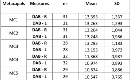
Metacapals Measures n= Mean SD
MC1 DAB - R 31 13,393 1,337 DAB - L 31 13,263 1,293 MC2 DAB - R 31 13,264 1,044 DAB - L 31 13,248 0,986 MC3 DAB - R 28 13,293 1,183 DAB - L 28 13,155 0,972 MC4 DAB - R 32 11,368 0,987 DAB - L 32 10,974 0,893 MC5 DAB - R 29 10,674 0,886 DAB - L 29 10,547 0,765
Table 14. Results of the means and standard deviation (SD) of the DAB measure for all MC. The highest SD is 1,337 and the lowest is 0,765.
Metacapals Measures n= Mean SD
MC1 DAH - R DAH - L 31 31 12,782 1,382 12,445 1,261 MC2 DAH - R 29 13,357 1,009 DAH - L 29 13,017 0,825 MC3 DAH - R 30 13,542 1,066 DAH - L 30 13,172 0,919 MC4 DAH - R 31 12,167 0,887 DAH - L 31 12,057 1,030 MC5 DAH - R 31 11,069 1,049 DAH - L 31 10,965 0,932
Table 15. Results of the means and standard deviation (SD) of the DAH measure for all MC. The highest SD is 1,382 and the lowest is 0,825.
34 The mean is important for our following test, the Two-sample paired test (T-test). The standard deviation (SD) can give us already some useful information about our data and our measures. The results are low for most of the measures. It means that the asymmetry is there but is not necessarily strong. For the majority of the measures; PMB, PMH, PAB, PAH, MB, MH, DMB, DAB and DAH; the SD is lower than 2, while for the ML and AL measures, the results are lower than 3 and higher than 2. We can already assess that there might have more asymmetry between the left and right sides in the ML and AL measures than the other measures.
Normality test
The next step was to do a normality test. It was important that our data was normal, it is better for the Two-sample paired test. The test we used was the Shapiro-Wilk. We applied the normality test to the measures of each right and left metacarpals, as for the descriptive statistics (Tables 16 to 20). That gave us one hundred and ten (110) p(value); of these, six were considered possibly not normal because there p(value) was p(<0.05). But we still considered them normal because the difference was not big (not lower than p(<0.01)). This result is not different enough to cause some anomaly in the results of the Two-sample paired test. However, five results had a p(<0.01), this may indicate that we have an individual with “strange” bones, and that it is reflected in our measurements. Because these bones exist and because we don’t want to force our data to be normal, we kept all the data. Moreover, these five results represent less than 0.05% of our data, which is minor. We considered that, because most of our values were parametric and normal, our data was parametric and normal.
35
Table 16. Normality test of Shapiro -Wilk for all the right (R) and left (L) of MC1, by
measures.
All results are considered normal.
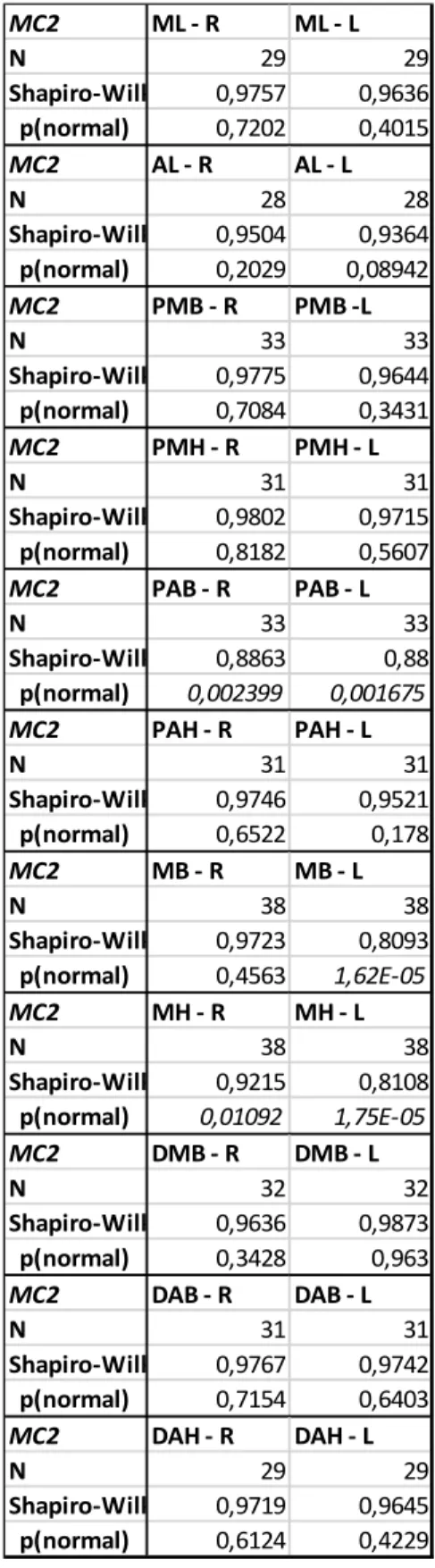
Table 17. Normality test of Shapiro -Wilk for all the right (R) and left (L) of MC2, by
measures.
PAB-L and R, MB-L, MH-L have a p(<0.01). MC1 ML - R ML - L N 31 31 Shapiro-Wilk W 0,9773 0,9565 p(normal) 0,7329 0,2344 MC1 AL - R AL - L N 29 29 Shapiro-Wilk W 0,9826 0,9673 p(normal) 0,8987 0,4896 MC1 PMB - R PMB -L N 30 30 Shapiro-Wilk W 0,9772 0,9525 p(normal) 0,7461 0,1967 MC1 PMH - R PMH - L N 27 27 Shapiro-Wilk W 0,9239 0,9674 p(normal) 0,0492 0,5341 MC1 PAB - R PAB - L N 31 31 Shapiro-Wilk W 0,9706 0,9626 p(normal) 0,5369 0,3403 MC1 PAH - R PAH - L N 28 28 Shapiro-Wilk W 0,9816 0,9513 p(normal) 0,8863 0,2134 MC1 MB - R MB - L N 37 37 Shapiro-Wilk W 0,971 0,9776 p(normal) 0,4350 0,6492 MC1 MH - R MH - L N 37 37 Shapiro-Wilk W 0,9768 0,9682 p(normal) 0,6193 0,3607 MC1 DMB - R DMB - L N 33 33 Shapiro-Wilk W 0,9768 0,9299 p(normal) 0,6851 0,0348 MC1 DAB - R DAB - L N 31 31 Shapiro-Wilk W 0,9803 0,9787 p(normal) 0,8201 0,7751 MC1 DAH - R DAH - L N 31 31 Shapiro-Wilk W 0,9557 0,9824 p(normal) 0,2236 0,8764 MC2 ML - R ML - L N 29 29 Shapiro-Wilk W 0,9757 0,9636 p(normal) 0,7202 0,4015 MC2 AL - R AL - L N 28 28 Shapiro-Wilk W 0,9504 0,9364 p(normal) 0,2029 0,08942 MC2 PMB - R PMB -L N 33 33 Shapiro-Wilk W 0,9775 0,9644 p(normal) 0,7084 0,3431 MC2 PMH - R PMH - L N 31 31 Shapiro-Wilk W 0,9802 0,9715 p(normal) 0,8182 0,5607 MC2 PAB - R PAB - L N 33 33 Shapiro-Wilk W 0,8863 0,88 p(normal) 0,002399 0,001675 MC2 PAH - R PAH - L N 31 31 Shapiro-Wilk W 0,9746 0,9521 p(normal) 0,6522 0,178 MC2 MB - R MB - L N 38 38 Shapiro-Wilk W 0,9723 0,8093 p(normal) 0,4563 1,62E-05 MC2 MH - R MH - L N 38 38 Shapiro-Wilk W 0,9215 0,8108 p(normal) 0,01092 1,75E-05 MC2 DMB - R DMB - L N 32 32 Shapiro-Wilk W 0,9636 0,9873 p(normal) 0,3428 0,963 MC2 DAB - R DAB - L N 31 31 Shapiro-Wilk W 0,9767 0,9742 p(normal) 0,7154 0,6403 MC2 DAH - R DAH - L N 29 29 Shapiro-Wilk W 0,9719 0,9645 p(normal) 0,6124 0,4229
36
Table 18. Normality test of Shapiro -Wilk for all the right (R) and left (L) of MC3, by
measures.
MB-L and MH-L have a p(<0.01).
Table 19. Normality test of Shapiro -Wilk for
all the right (R) and left (L) of MC4, by measures.
All results are considered normal. MC3 ML - R ML - L N 31 31 Shapiro-Wilk W 0,9847 0,9665 p(normal) 0,9256 0,4278 MC3 AL - R AL - L N 31 31 Shapiro-Wilk W 0,9616 0,9604 p(normal) 0,3222 0,2998 MC3 PMB - R PMB -L N 36 36 Shapiro-Wilk W 0,9839 0,9816 p(normal) 0,8668 0,7991 MC3 PMH - R PMH - L N 35 35 Shapiro-Wilk W 0,9235 0,9723 p(normal) 0,01801 0,5098 MC3 PAB - R PAB - L N 34 34 Shapiro-Wilk W 0,9554 0,9735 p(normal) 0,1777 0,5647 MC3 PAH - R PAH - L N 33 33 Shapiro-Wilk W 0,9864 0,9765 p(normal) 0,9444 0,6776 MC3 MB - R MB - L N 38 38 Shapiro-Wilk W 0,9695 0,8693 p(normal) 0,3792 0,0003862 MC3 MH - R MH - L N 38 38 Shapiro-Wilk W 0,9781 0,6302 p(normal) 0,6499 1,47E-08 MC3 DMB - R DMB - L N 28 28 Shapiro-Wilk W 0,9846 0,9556 p(normal) 0,9429 0,2722 MC3 DAB - R DAB - L N 28 28 Shapiro-Wilk W 0,9624 0,956 p(normal) 0,3971 0,2789 MC3 DAH - R DAH - L N 30 30 Shapiro-Wilk W 0,9645 0,9728 p(normal) 0,4013 0,6173 MC4 ML - R ML - L N 31 31 Shapiro-Wilk W 0,9656 0,9692 p(normal) 0,4079 0,4979 MC4 AL - R AL - L N 31 31 Shapiro-Wilk W 0,9504 0,9572 p(normal) 0,1599 0,2454 MC4 PMB - R PMB -L N 38 38 Shapiro-Wilk W 0,9713 0,9626 p(normal) 0,4292 0,2312 MC4 PMH - R PMH - L N 35 35 Shapiro-Wilk W 0,9496 0,9857 p(normal) 0,1105 0,9189 MC4 PAB - R PAB - L N 34 34 Shapiro-Wilk W 0,9587 0,982 p(normal) 0,2233 0,8346 MC4 PAH - R PAH - L N 31 31 Shapiro-Wilk W 0,9722 0,9579 p(normal) 0,5821 0,257 MC4 MB - R MB - L N 39 39 Shapiro-Wilk W 0,9666 0,9626 p(normal) 0,2936 0,2177 MC4 MH - R MH - L N 39 39 Shapiro-Wilk W 0,9798 0,9551 p(normal) 0,6954 0,1216 MC4 DMB - R DMB - L N 33 33 Shapiro-Wilk W 0,9668 0,96 p(normal) 0,3984 0,2577 MC4 DAB - R DAB - L N 32 32 Shapiro-Wilk W 0,9713 0,9315 p(normal) 0,5372 0,04324 MC4 DAH - R DAH - L N 31 31 Shapiro-Wilk W 0,9875 0,9542 p(normal) 0,9691 0,2037
37
Table 20. Normality test of Shapiro -Wilk for all the right (R) and left (L) MC5, by measures.
All results are considered normal. MC5 ML - R ML - L N 32 32 Shapiro-Wilk W 0,9343 0,9671 p(normal) 0,05168 0,4239 MC5 AL - R AL - L N 30 30 Shapiro-Wilk W 0,9738 0,9611 p(normal) 0,6472 0,3298 MC5 PMB - R PMB -L N 37 37 Shapiro-Wilk W 0,9833 0,98 p(normal) 0,8397 0,7314 MC5 PMH - R PMH - L N 35 35 Shapiro-Wilk W 0,983 0,9823 p(normal) 0,8526 0,8305 MC5 PAB - R PAB - L N 36 36 Shapiro-Wilk W 0,9764 0,981 p(normal) 0,6226 0,7798 MC5 PAH - R PAH - L N 36 36 Shapiro-Wilk W 0,9618 0,9591 p(normal) 0,2433 0,2018 MC5 MB - R MB - L N 37 37 Shapiro-Wilk W 0,9678 0,9579 p(normal) 0,3517 0,1727 MC5 MH - R MH - L N 37 37 Shapiro-Wilk W 0,9763 0,9877 p(normal) 0,6024 0,9486 MC5 DMB - R DMB - L N 33 33 Shapiro-Wilk W 0,9719 0,983 p(normal) 0,5358 0,8707 MC5 DAB - R DAB - L N 29 29 Shapiro-Wilk W 0,9792 0,9774 p(normal) 0,8176 0,7689 MC5 DAH - R DAH - L N 31 31 Shapiro-Wilk W 0,9165 0,9748 p(normal) 0,01905 0,6592
38 Two-sample paired test
The Two-sample paired test (T-test) was our most important test. It is with the results of this one that we could mostly interpret our data and then answer most of our questions and hypotheses.
As mentioned previously, we had one hundred and ten (110) groups, one for each metacarpal’s side and measure. We compared the means of the groups, two by two according to the side. For example, the mean of all ML-R of the MC1 was compared with the mean of all ML-L of the MC1. So, we obtained fifty-five (55) results. These results are composed of a T-test and a p(same mean) (or p(value)). It is the latter that is more meaningful in the interpretation of the data. Like for the normality test, the p(<0.05) is an indicator, it allows us to reject or not the null hypothesis.
As said previously, our null hypothesis was:
There is no statistically significant difference between the measures of the left and the right sides for each metacarpal.
For each of the fifty-five (55) results, we asked if p(<0.05). If the answer was yes, we refuted the null hypothesis. The results we obtained can be differently explained according of the way we compared the data; between the measures (Tables 21 to 31) or between the metacarpals (Table 32).
39 Metacapals Measures n= Mean T-test p (same mean) <0,05=
MC1 ML - R 31 42,614 2,4086 0,022365 Yes ML - L 31 42,291 MC2 ML - R 29 63,346 2,5329 0,017199 Yes ML - L 29 62,901 MC3 ML - R 31 62,394 2,8575 0,0076872 Yes ML - L 31 61,709 MC4 ML - R 31 53,503 3,6904 0,00088733 Yes ML - L 31 52,989 MC5 ML - R 32 50,278 2,7774 0,0092153 Yes ML - L 32 49,715
Table 21. Results of the Two-sample paired test (T-test) of the ML measure for all MC. All results are p(<0.05).
Metacapals Measures n= Mean T-test p (same mean) <0,05=
MC1 AL - R 29 40,751 2,0718 0,047611 Yes AL - L 29 40,474 MC2 AL - R 28 60,891 5,1617 0,000019725 Yes AL - L 28 60,182 MC3 AL - R AL - L 31 31 58,478 58,046 3,1526 0,0036585 Yes MC4 AL - R 31 52,819 2,8157 0,0085193 Yes AL - L 31 52,44 MC5 AL - R 30 49,654 3,3728 0,0021257 Yes AL - L 30 49,192
Table 22. Results of the Two-sample paired test (T-test) of the AL measure for all MC. All results are p(<0.05).
Metacapals Measures n= Mean T-test p (same mean) <0,05=
MC1 PMB - R 30 15,276 4,4183 0,00012722 Yes PMB - L 30 14,782 MC2 PMB - R 33 17,303 -0,15971 0,87411 No PMB - L 33 17,328 MC3 PMB - R 36 14,242 1,8513 0,072575 No PMB - L 36 13,823 MC4 PMB - R 38 11,81 -0,296 0,76889 No PMB - L 38 11,846 MC5 PMB - R 37 13,424 0,42108 0,42108 No PMB - L 37 13,358
Table 23. Results of the Two-sample paired test (T-test) of the PMB measure for all MC. Results showed that MC1 have p(<0.05).
40 Metacapals Measures n= Mean T-test p (same mean) <0,05=
MC1 PMH - R 27 15,075 3,024 0,0055522 Yes PMH - L 27 14,544 MC2 PMH - R 31 15,79 -0,8815 0,38506 No PMH - L 31 15,904 MC3 PMH - R 35 15,529 -0,58836 0,56018 No PMH - L 35 15,663 MC4 PMH - R 35 12,154 3,8165 0,00054615 Yes PMH - L 35 11,706 MC5 PMH - R 35 11,451 1,5344 0,1342 No PMH - L 35 11,196
Table 24. Results of the Two-sample paired test (T-test) of the PMH measure for all MC. Results showed that MC1 and MC4 have a p(<0.05).
Metacapals Measures n= Mean T-test p (same mean) <0,05=
MC1 PAB - R 31 13,334 2,6265 0,013455 Yes PAB - L 31 12,797 MC2 PAB - R 33 10,432 -0,93053 0,35907 No PAB - L 33 10,708 MC3 PAB - R 34 10,289 2,0651 0,046844 Yes PAB - L 34 9,9576 MC4 PAB - R 34 6,8041 1,1734 0,24903 No PAB - L 34 6,61 MC5 PAB - R 36 9,2467 3,7385 0,00066046 Yes PAB - L 36 8,7039
Table 25. Results of the Two-sample paired test (T-test) of the PAB measure for all MC. Results showed that MC1, MC3 and MC5 have a p(<0.05).
Metacapals Measures n= Mean T-test p (same mean) <0,05=
MC1 PAH - R PAH - L 28 28 10,711 10,576 0,68934 0,49649 No MC2 PAH - R 31 13,695 -0,22894 0,82047 No PAH - L 31 13,738 MC3 PAH - R 33 13,52 1,3304 0,19278 No PAH - L 33 13,211
MC4 PAH - R PAH - L 31 31 9,3197 8,6287 3,1375 0,0038029 Yes
MC5 PAH - R 36 9,93 0,04296 0,96598 No
PAH - L 36 9,9233
Table 26. Results of the Two-sample paired test (T-test) of the PAH measure for all MC. Results showed that MC4 have a p(<0.05).
41 Metacapals Measures n= Mean T-test p (same mean) <0,05=
MC1 MB - R 37 11,873 3,6319 0,00086906 Yes MB - L 37 11,56 MC2 MB - R 38 8,2918 1,661 0,10516 No MB - L 38 8,0429 MC3 MB - R 38 8,1729 -2,29 0,02782 Yes MB - L 38 8,3879 MC4 MB - R 39 6,6267 1,309 0,1984 No MB - L 39 6,5538 MC5 MB - R 37 7,53 2,7897 0,0083824 Yes MB - L 37 7,3116
Table 27. Results of the Two-sample paired test (T-test) of the MB measure for all MC. Results showed that MC1, MC3 and MC5 have a p(<0.05).
Metacapals Measures n= Mean T-test p (same mean) <0,05=
MC1 MH - R 37 8,2376 0,23554 0,81512 No MH - L 37 8,222 MC2 MH - R 38 8,8745 -0,74137 0,46315 No MH - L 38 8,9784 MC3 MH - R 38 9,1258 0,51256 0,61131 No MH - L 38 9,0161 MC4 MH - R 39 7,5762 0,41423 0,68103 No MH - L 39 7,5379 MC5 MH - R 37 6,8186 0,65692 0,51541 No MH - L 37 6,7759
Table 28. Results of the Two-sample paired test (T-test) of the MH measure for all MC. Results showed that no MC have a p(<0.05).
Metacapals Measures n= Mean T-test p (same mean) <0,05=
MC1 DMB - R DMB - L 33 33 15,461 15,269 1,3606 0,18315 No MC2 DMB - R 32 14,576 2,4965 0,018069 Yes DMB - L 32 14,386 MC3 DMB - R 28 14,546 2,7199 0,01128 Yes DMB - L 28 14,225 MC4 DMB - R DMB - L 33 33 12,732 12,409 3,4555 0,0015705 Yes MC5 DMB - R 33 11,865 4,0238 0,00032758 Yes DMB - L 33 11,569
Table 29. Results of the Two-sample paired test (T-test) of the DMB measure for all MC. Results showed that MC2, MC3, MC4 and MC5 have a p(<0.05).
42 Metacapals Measures n= Mean T-test p (same mean) <0,05=
MC1 DAB - R 31 13,393 1,1199 0,27165 No DAB - L 31 13,263 MC2 DAB - R 31 13,264 0,14798 0,88335 No DAB - L 31 13,248 MC3 DAB - R 28 13,293 0,9464 0,35234 No DAB - L 28 13,155 MC4 DAB - R 32 11,368 2,9304 0,0063043 Yes DAB - L 32 10,974 MC5 DAB - R 29 10,674 1,1434 0,26254 No DAB - L 29 10,547
Table 30. Results of the Two-sample paired test (T-test) of the DAB measure for all MC. Results showed that MC4 have a p(<0.05).
Metacapals Measures n= Mean T-test p (same mean) <0,05=
MC1 DAH - R 31 12,782 2,096 0,04462 Yes DAH - L 31 12,445 MC2 DAH - R 29 13,357 3,0041 0,0055602 Yes DAH - L 29 13,017 MC3 DAH - R 30 13,542 2,7829 0,0093794 Yes DAH - L 30 13,172 MC4 DAH - R 31 12,167 0,75051 0,45879 No DAH - L 31 12,057 MC5 DAH - R 31 11,069 1,0824 0,28772 No DAH - L 31 10,965
Table 31. Results of the Two-sample paired test (T-test) of the DAH measure for all MC. Results showed that MC1, MC2 and MC3 have a p(<0.05).
43
Graph 1. Bar graph of the results from the Two-sample paired test (T-test) for each metacarpal. X = Measure. Y = p (same mean).
The results under the line are p (<0,05) and express significant difference.
By measures, between the five metacarpals, our outcome showed that the ML and the AL measures clearly demonstrate that there is a statistically significant difference between the right and the left metacarpals, for each of the metacarpal bones because all of their p(same mean) correspond to p(<0.05). We can also consider that the DMB measure showed that there is a strong possibility that there is a statistically significant difference between the right and the left metacarpals, although p(same mean) of the MC1 does not correspond to p(<0.05). Concerning the PAB, MB and DAH measures, the results showed that there is statistically significant difference for three of the five metacarpals, however because not all the results have this difference, we cannot assert that difference, as for the PMB, PMH, PAH, MH and DAB measurements. These measures have between two and zero metacarpals that have a p(same mean) corresponding to p(<0.05), consequently we consider that the analysis showed that there is not a statistically significant difference between the right and the left metacarpals (Graph 1).
We can assert that there is a statistically significant difference between the right and the left metacarpals when we take these measures: ML and AL. These are the