Bauwens : CORE and Department of Economics, Université Catholique de Louvain Preminger : Department of Economics, University of Haifa, 31905 Israel
Rombouts : Institute of Applied Economics at HEC Montréal, CIRANO, CIRPEE, CREF, CORE (Université Catholique de Louvain), CREF 3000, chemin de la Côte-Sainte-Catherine, Montréal (Québec) Canada H3T 2A7 Bauwens’ work was supported by a FSR grant from UCL. He is also a member of ECORE, a newly created association between ECARES and CORE. Arie Preminger acknowledges the financial support provided through the European Community’s Human Potential Programme under contract HPRN-CT-2002-00232, Microstructure of Financial Markets in Europe, and the Ernst Foundation. This text presents research results of the Belgian Program on Interuniversity Poles of Attraction initiated by the Belgian State, Prime Minister’s Office, Science Policy Programming. The scientific responsibility is assumed by the authors.
Cahier de recherche/Working Paper 07-33
Theory and Inference for a Markov-Switching GARCH Model
Luc Bauwens
Arie Preminger
Jeroen V.K. Rombouts
Abstract:
We develop a Markov-switching GARCH model (MS-GARCH) wherein the
conditional mean and variance switch in time from one GARCH process to another.
The switching is governed by a hidden Markov chain. We provide sufficient
conditions for geometric ergodicity and existence of moments of the process.
Because of path dependence, maximum likelihood estimation is not feasible. By
enlarging the parameter space to include the state variables, Bayesian estimation
using a Gibbs sampling algorithm is feasible. We illustrate the model on SP500 daily
returns.
Keywords: GARCH, Markov-switching, Bayesian inference
Résumé:
Nous développons un modèle de changement de régime markovien GARCH où la
moyenne et la variance conditionnelle change dans le temps. Nous proposons des
conditions suffisantes pour l’ergodicité géométrique et l’existence des moments du
processus. Nous estimons le modèle en utilisant l’inférence Bayesienne. Nous
illustrons le modèle avec des données quotidiennes de SP500.
Mots clés: GARCH, Changement de régime markovien, Inférence Bayesienne
1
Introduction
The volatility of financial markets has been the object of numerous developments and ap-plications over the past two decades, both theoretically and empirically. In this respect, the most widely used class of models is certainly that of GARCH models (see e.g. Bollerslev, Engle, and Nelson (1994) for an overview). These models usually indicate a high persistence of the conditional variance (i.e. a nearly integrated GARCH process). Diebold (1986) and Lamoureux and Lastrapes (1990), among others, argue that the nearly integrated behavior of the conditional variance may originate from structural changes in the variance process which are not accounted for by standard GARCH models. Furthermore, Mikosch and Starica (2004) show that estimating a GARCH model on a sample displaying structural changes in the un-conditional variance does indeed create an integrated GARCH effect. These findings clearly indicate a potential source of misspecification, to the extent that the form of the conditional variance is relatively inflexible and held fixed throughout the entire sample period. Hence the estimates of a GARCH model may suffer from a substantial upward bias in the persistence parameter. Therefore, models in which the parameters are allowed to change over time may be more appropriate for modelling volatility.
Indeed, several models based on the idea of regime changes have been proposed. Schwert (1989) consider a model in which returns can have a high or low variance, and switches between these states are determined by a two state Markov process. Hamilton and Susmel (1994) and Cai (1994) introduce an ARCH model with Markov-switching parameters in order to take into account sudden changes in the level of the conditional variance. They use an ARCH specification instead of a GARCH to avoid the problem of path dependence of the conditional variance which renders the computation of the likelihood function infeasible. This occurs because the conditional variance at time t depends on the entire sequence of regimes up to time t due to the recursive nature of the GARCH process. Since the regimes are unobservable, one needs to integrate over all possible regime paths when computing the sample likelihood, but the number of possible paths grows exponentially with t, which renders ML estimation intractable. Gray (1996) presents a tractable Markov-switching GARCH model and a modification of his model is suggested by Klaassen (2002); see also Bollen, Gray, and Whaley (2000), Dueker (1997), Haas, Mittnik, and Paolella (2004), and Marcucci (2005) for related papers. Stationarity conditions for some of these tractable models are given by
Abramson and Cohen (2007).
The objective of this paper is to develop both the probabilistic properties and the estima-tion of a Markov swtiching GARCH (MS-GARCH) model that has a finite number of regimes in each of which the conditional mean is constant and the conditional variance takes the form of a GARCH(1,1) process. We provide sufficient conditions for the geometric ergodicity and the existence of moments of the proposed model. We find that for strict stationarity, it is not necessary that the stability condition of Nelson (1990) be satisfied in all the GARCH regimes but it must be satisfied on average with respect to the unconditional probabilities of the regimes. Further, for covariance stationarity, the GARCH parameters in some regimes can be integrated or even explosive.
Concerning the estimation method, we propose a Bayesian Markov chain Monte Carlo (MCMC) algorithm that circumvents the problem of path dependence by including the state variables in the parameter space and simulating them by Gibbs sampling. We illustrate by a simulation experiment that the algorithm is able to recover the parameters of the data generating process, and we apply the algorithm to a real data set. For the more simple MS-ARCH case, Francq, Roussignol, and Zakoian (2001) establish the consistency of the ML estimator. Bayesian estimation of a Markov switching ARCH model where only the constant in the ARCH equation can switch, as in Cai (1994), has been studied and illustrated by Kaufman and Fruhwirth-Schnatter (2002) and Kaufman and Scheicher (2006). Das and Yoo (2004) propose an MCMC algorithm for the same model (switch in the constant only) but with a GARCH term and therefore tackle the path dependence problem, but they do not provide an application to a real data series. Finally, the most comparable work to our paper (for estimation) is that of Henneke, Rachev, and Fabozzi (2006) who estimate by a MCMC algorithm a Markov-switching ARMA-GARCH model. They apply their algorithm to the data used by Hamilton and Susmel (1994). Non-Bayesian estimation of MS-GARCH models is studied by Francq and Zakoian (2005) who propose to estimate the model by the generalized method of moments.
This sequel of the paper is organized as follows: in Section 2, we define our version of the MS-GARCH model and state sufficient conditions for geometric ergodicity and existence of moments. In Section 3, we explain how the model can be estimated in the Bayesian framework and provide a numerical example. In Section 4, we apply our approach to financial data. and
in Section 5 we conclude and discuss possible extensions. Proofs of the theorems stated in the paper are gathered in an appendix.
2
Markov-Switching GARCH Model
The GARCH(1,1) model can be defined by
yt = µt+ σtut (1)
σ2t = ω + α²2t−1+ βσ2t−1 (2)
where σt and µt are measurable functions of yt−τ for τ ≤ t − 1, ²t = yt− µt, and the error
term ut is i.i.d. with zero mean and unit variance. In order to ensure easily the positivity of the conditional variance we impose the restrictions ω > 0, α ≥ 0 and β ≥ 0. For simplicity, we assume that µt is constant. The sum α + β measures the persistence of a shock to the conditional variance in equation (2). When a GARCH model is estimated using daily or higher frequency data, the estimate of this sum tends to be close to one, indicating that the volatility process is highly persistent and the second moment of the return process may not exist. However it was argued that the high persistence may artificially result from regime shifts in the GARCH parameters over time, see Diebold (1986), Lamoureux and Lastrapes (1990), and Mikosch and Starica (2004), among others.
This motivates our idea to estimate a model that permits regime switching in the param-eters. We call it a Markov-switching GARCH (MS-GARCH) model. It is a generalization of the GARCH model and permits a different persistence in the conditional variance of each regime. Thus, the conditional variance in each regime accommodates volatility clustering, nesting the GARCH model as special case. Let {st} be an ergodic Markov chain on a finite
set S = {1, . . . , n}, with transition probabilities {ηij = P(st = i|st−1 = j)} and invariant
probability measure {πi}. The MS-GARCH model is given by
yt = µst+ σtut (3)
σ2t = ωst + αst²2t−1+ βstσt−12 (4)
where ωst > 0, αst ≥ 0, βst ≥ 0 for st ∈ {1, 2, . . . n}, and ²t = yt− µst. These
assump-tions on the GARCH coefficients entail that σ2
t is almost surely strictly positive. Conditions
GARCH(p,q) model with zero means µst, in which the discrete Markov chain of the latent
states is initiated from its stationary probabilities, have been derived by Francq and Zakoian (2005), see also Francq, Roussignol, and Zakoian (2001). In related papers, Yang (2000), Yao and Attali (2000), Yao (2001), and Francq and Zakoian (2002) derived conditions for the asymptotic stationarity of some AR and ARMA models with Markov-switching regimes. The MS-GARCH process is not a Markov chain in general. However, the extended process Zt = (yt, ht, st)0 is a Markov chain (see the Appendix). In what follows, we state mild
regularity conditions for which this chain is geometrically ergodic and has finite moments. These results are based on Markov chain theory, see e.g. Meyn and Tweedie (1993) and Chan (1993). We impose the following assumptions:
A1 The error term ut is i.i.d. with a continuous density on the whole real line which is
centered on zero. Furthermore, E(|u2
t|δ) < ∞ for some δ > 0.
A2 αi> 0, βi> 0 and ηii∈ (0, 1) for i ∈ {1, . . . , n}. A3 Pn
i=1
πiE[log(αiu2t + βi)] < 0.
The first assumption is satisfied for a wide range of distributions for the error term, e.g. the normal and the Student distributions. For δ = 1, we set the variance to unity and if δ < 1, the parameters of the conditional scaling factor of the data are estimated. The second assumption is slightly stronger than the non-negativity conditions of Bollerslev (1986) for the GARCH(1,1) model. Under this assumption all the regimes are accessible and the discrete Markov chain is ergodic. These assumptions are needed in order to establish the irreducibility and aperiodicity of the process. Assumption A3 implies that at least one of the regimes is stable. We assume, without loss of generality throughout that in the first regime (st= 1) the process is strictly stationary, thus E log(α1u2t + β1) < 0. To obtain the results in Theorem 1,
we observe that it is not necessary that the strict stationarity requirement of Nelson (1990) be satisfied for all the GARCH regimes but on average with respect to the invariant probability distribution of the latent states.
Theorem 1 Under assumptions A1-A3, yt is geometrically ergodic and if it is initiated from
its stationary distribution, then the process is strictly stationary and β-mixing (absolutely regular) with exponential decay. Moreover, E(|yt|2p) < ∞ for some p ∈ (0, δ] where the
The geometric ergodicity ensures not only that a unique stationary probability measure for the process exists, but also that the chain, irrespective of its initialization, converges to it at a geometric rate with respect to the total variation norm. Markov chains with this property satisfy conventional limit theorems such as the law of large numbers and the central limit theorem for any given starting value given the existence of suitable moments, see Meyn and Tweedie (1993, ch.17) for details. The definition of regular mixing can be found in Doukhan (1994, Section 1.1) who also shows that the exponential decaying rate of the mixing numbers implies that the autocovariance function converges to zero at least at the same rate. In order to establish the existence of higher order moments, we define the n × n matrix
Ω = E(α1u2t + β1)kη11 · · · E(αnu2t+ βn)kηn1 .. . . .. ... E(α1u2t + β1)kη1n · · · E(αnu2t+ βn)kηnn .
A similar matrix was first introduced by Yao and Attali (2000) for nonlinear autoregressive models with Markov switching. Let ρ(·) denote the spectral radius of a matrix, i.e. its largest eigenvalue in modulus. Then, we impose the following conditions:
A4 E(|u2
t|k) < ∞ for some integer k ≥ 1.
A5 ρ(Ω) < 1.
Theorem 2 Under assumptions A1-A2 and A4-A5, the process is geometrically ergodic and E(|y2
t|k) < ∞ for some integer k ≥ 1, where the expectations are taken under the stationary
distribution.
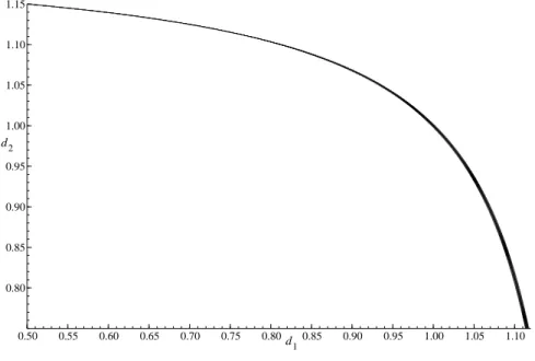
The spectral radius condition used in Theorem 2 is simple to check in the leading case where k = 1. Let di = αi + βi: if di < 1, assumption A5 is satisfied for this case, since ηij ∈ (0, 1), see Lutkepohl (1996, p. 141, 4(b)), and the resulting MS-GARCH process is
covariance-stationary. However, it is not necessary that all the GARCH processes of each regime be covariance-stationary. To illustrate this, we plot in Figure 1 the boundary curve ρ(Ω) = 1 for n = 2 where η11= η22= 0.85. The covariance-stationarity region is the interior intersection of the boundary curve and the two axes. We observe that one of the GARCH
regimes does not need to be weakly stationary and can even be mildly explosive, provided that the other regime is sufficiently stable.
0.50 0.55 0.60 0.65 0.70 0.75 0.80 0.85 0.90 0.95 1.00 1.05 1.10 0.80 0.85 0.90 0.95 1.00 1.05 1.10 1.15 d1 d2
Figure 1: Stationarity region for two-state MS-GARCH with transition probabilities η11 =
η22= 0.85 and di= αi+ βi
As a special case, we consider a situation where we start the discrete Markov chain from its invariant distribution. This case is equivalent to a regime switching GARCH model where the probabilities are constant over time, see Bauwens, Preminger, and Rombouts (2006). Under assumptions A1-A2, it can be shown that a sufficient condition for geometric ergodictiy and existence of moments is given byPnj=1πjE(αju2t + βj)k< 1. We observe that the condition
derived by Bollerslev (1986) for covariance-stationarity under a single GARCH model need not hold in each regime but for the weighted average of the GARCH parameters. Note, that high values of the parameters of the non-stable GARCH processes must be compensated by low probabilities for their regimes.
3
Estimation
Given the current computing capabilities, the estimation of switching GARCH models by the maximum likelihood method is impossible, since the conditional variance depends on the whole past history of the state variables. We tackle the estimation problem by Bayesian
inference, which allows us to treat the latent state variables as parameters of the model and to construct the likelihood function assuming we know the states. This technique is called data augmentation, see Tanner and Wong (1987) for the basic principle and more details. In Section 3.1, we present the Bayesian algorithm for the case of two regimes, and in Section 3.2, we illustrate that it recovers correctly the parameters of a simulated data generating process.
3.1 Bayesian Inference
We explain the Bayesian algorithm for a MS-GARCH model with two regimes and normality of the error term ut. The normality assumption is a natural starting point. A more flexible
distribution, such as the Student distribution, could be considered, although one may be skeptical that this is needed since Gray (1996) reports large and imprecise estimates of the degrees of freedom parameters.
For the case of two regimes, the model is given by equations (3)-(4), st= 1 or 2 indicating
the active regime. We denote by Yt the vector (y1y2 . . . yt) and likewise St = (s1s2 . . . st).
The model parameters consist of η = (η11, η21, η12, η22)0, µ = (µ
1, µ2)0, and θ = (θ10, θ20)0, where
θk = (ωk, αk, βk)0 for k = 1, 2. The joint density of yt and st given the past information and
the parameters can be factorized as
f (yt, st|µ, θ, η, Yt−1, St−1) = f (yt|st, µ, θ, Yt−1, St−1)f (st|η, Yt−1, St−1). (5)
The conditional density of yt is the Gaussian density
f (yt|st, µ, θ, Yt−1, St−1) = p 1 2πσ2 t exp µ −(yt− µst)2 2σ2 t ¶ (6) where σ2
t, defined by equation (4), is a function of θ. The marginal density (or probability
mass function) of st is specified by
f (st|η, Yt−1, St−1) = f (st|η, st−1) = ηstst−1 (7) with η11+ η21 = 1, η12+ η22 = 1, 0 < η11 < 1 and 0 < η22< 1. This specification says that
st depends only on the last state and not on the previous ones and on the past observations
of yt, so that the state process is a first order Markov chain with no absorbing state.
The joint density of y = (y1, y2, . . . , yT) and S = (s1, s2, . . . , sT) given the parameters is
then obtained by taking the product of the densities in (6) and (7) over all observations: f (y, S|µ, θ, η) ∝ T Y t=1 σ−1t exp µ −(yt− µst)2 2σ2 t ¶ ηstst−1. (8)
Since integrating this function with respect to S by summing over all paths of the state variables is numerically too demanding, we implement a Gibbs sampling algorithm that allows us to sample from the full conditional posterior densities of blocks of parameters given by θ, µ, η, and the elements of S. We explain what are our prior densities for θ, µ, and η when we define the different blocks of the Gibbs sampler.
3.1.1 Sampling st
To sample st we must condition on st−1 and st+1 (because of the Markov chain for the states) and on the future state variables (st+1, st+2, . . . sT) (because of path dependence of
the conditional variances). The full conditional mass function of state t is ϕ(st|S6=t, µ, θ, η, y) ∝ η1,s2−st−1t η st−1 2,st−1η 2−st+1 1,st η st+1−1 2,st T Y j=t σj−1exp à −(yj− µsj)2 2σ2 j ! (9) where we can replace η2,st−1 by 1 − η1,st−1 and η2,st by 1 − η1,st. Since sttakes two values, it
is easy to simulate this discrete distribution. 3.1.2 Sampling η
Given a prior density π(η),
ϕ(η|S, µ, θ, y) ∝ π(η)
T
Y
t=1
ηstst−1 (10)
which does not depend on µ, θ and y. For simplicity, we can work with η11 and η22 as free
parameters and assign to each of them a beta prior density on (0, 1). The posterior densities are then also independent beta densities. For example,
ϕ(η11|S) ∝ η11a11+n11−1(1 − η11)a21+n21−1 (11)
where a11 and a21 are the parameters of the beta prior, n11 is the number of times that
st = st−1 = 1 and n21 is the number of times that st = 2 and st−1= 1. A uniform prior on
(0, 1) corresponds to a11= a21= 1.
3.1.3 Sampling θ Given a prior density π(θ),
ϕ(θ|S, µ, η, y) ∝ π(θ) T Y t=1 σ−1t exp µ −(yt− µst)2 2σ2 t ¶ , (12)
which does not depend on η. We sample θ by the griddy-Gibbs sampler. The algorithm works as follows at iteration r +1, given draws at iteration r denoted by the superscript (r) attached to the parameters:
1. Using (12), compute κ(ω1|S(r), β(r)1 , α(r)1 , θ(r)2 , µ(r), y), the kernel of the conditional
pos-terior density of ω1 given the values of S, β1, α1, θ2, and µ sampled at iteration r, over a grid (ω1
1, ω12· · · , ωG1), to obtain the vector Gκ= (κ1, κ2, · · · , κG).
2. By a deterministic integration rule using M points, compute Gf = (0, f2, . . . , fG) where
fi = Z ωi 1 ω1 1 κ(ω1|S(r), β1(r), α(r)1 , θ(r)2 , µ(r), y) dω1, i=2,...,G. (13)
3. Generate u ∼ U (0, fG) and invert f (ω1|S(r), β(r)
1 , α(r)1 , θ(r)2 , µ(r), y) by numerical
inter-polation to get a draw ω1(r+1)∼ ϕ(ω1|S(r), β1(r), α(r)1 , θ(r)2 , µ(r), y).
4. Repeat steps 1-3 for ϕ(β1|S(r), ω1(r+1), α(r)1 , θ2(r), µ(r), y),
ϕ(α1|S(r), ω(r+1) 1 , β (r+1) 1 , θ (r) 2 , µ(r), y), ϕ(ω2|S(r), β2(r), α (r) 2 , θ (r+1) 1 , µ(r), y), etc.
Note that intervals of values for the elements of θ1 and θ2 must be defined. The choice of
these bounds (such as ω1
1 and ωG1) needs to be fine tuned in order to cover the range of the
parameter over which the posterior is relevant. Over these intervals, the prior can be chosen as we wish, for example as uniform densities.
3.1.4 Sampling µ Given a prior density π(µ),
ϕ(µ|S, θ, η, y) ∝ π(µ) T Y t=1 σt−1exp µ −(yt− µst)2 2σ2 t ¶ (14) which does not depend on η. It is not possible to factorize this function into the product of a function that depends on µ1 but not on µ2, and another one that depends on µ2 but not on µ1. Moreover, since σt depends on µ1 or µ2 (depending on t), the analytical form of the
likelihood as a function of µ1 or µ2 is not a known density (e.g. a normal). Hence we must
sample µ1 and µ2 jointly and numerically. We use the griddy-Gibbs sampler and we factorize
3.2 Simulation Example
We have simulated a data generating process (DGP) corresponding to the model defined by equations (3)-(4) for two states, and ut∼ N (0, 1). The parameter values are reported in Table
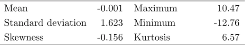
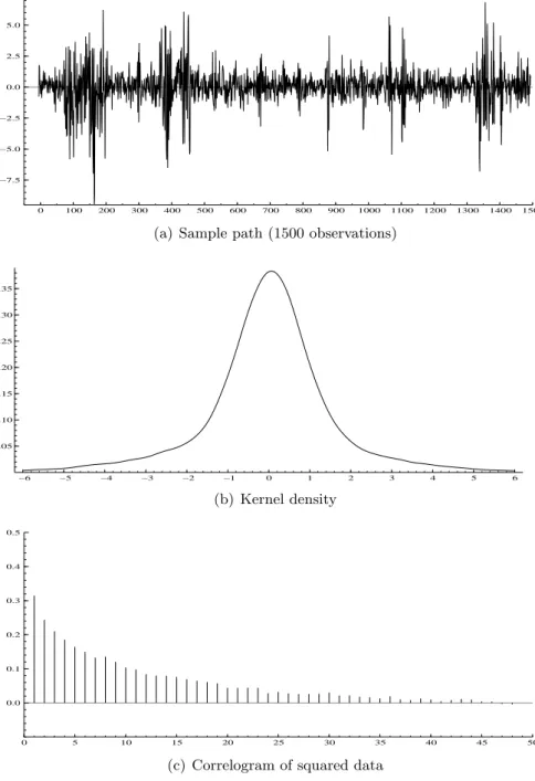
2. The second GARCH equation implies a higher and more persistent conditional variance than the first one. The other parameter values are inspired by previous empirical results, like in Hamilton and Susmel (1994), and our results presented in the next section. In particular, the transition probabilities of staying in each regime are close to unity. All the assumptions for stationarity and existence of moments of high order are satisfied by this DGP. In Table 1, we report some summary statistics for 50,000 observations from this DGP, and in Figure 2, we show the 1,500 initial observations of the series, and based on the 50,000 observations, the estimated density of the data and the autocorrelations of the squared data. The mean of the data is close to zero. The density is slightly skewed to the left, and its excess kurtosis is estimated to be 3.57 (the excess kurtosis is 1.62 for the first component GARCH and 0.12 for the second). The ACF of the squared data is strikingly more persistent than the ACF of each GARCH component, which are both virtually at 0 after 10 lags. Said differently, a GARCH(1,1) process would have to be close to integrated to produce the excess kurtosis and the ACF shown in Figure 2.
Table 1: Descriptive statistics for 50000 simulated data
Mean -0.001 Maximum 10.47
Standard deviation 1.623 Minimum -12.76
Skewness -0.156 Kurtosis 6.57
Statistics for 50,000 observations of the DGP defined in Table 2.
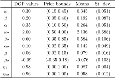
In Table 2, we report the posterior means and standard deviations for the model corre-sponding to the DGP, using the first 1,500 observations of the simulated data described above and shown in panel (a) of Figure 2. The results are in the last two columns of the table. In Figure 3, we report the corresponding posterior densities. The prior density of each parameter is uniform between the bounds reported in Table 2 with the DGP values. Thus, these bounds were used for the integrations in the griddy-Gibbs sampler (except for η11and η22 since they
0 100 200 300 400 500 600 700 800 900 1000 1100 1200 1300 1400 1500 −7.5 −5.0 −2.5 0.0 2.5 5.0
(a) Sample path (1500 observations)
−6 −5 −4 −3 −2 −1 0 1 2 3 4 5 6 0.05 0.10 0.15 0.20 0.25 0.30 0.35 (b) Kernel density 0 5 10 15 20 25 30 35 40 45 50 0.0 0.1 0.2 0.3 0.4 0.5
(c) Correlogram of squared data
Table 2: Posterior means and standard deviations (simulated DGP) DGP values Prior bounds Means St. dev.
ω1 0.30 (0.15 0.45) 0.345 (0.051) β1 0.20 (0.05 0.40) 0.192 (0.087) α1 0.35 (0.10 0.50) 0.264 (0.051) ω2 2.00 (0.50 4.00) 2.136 (0.688) β2 0.60 (0.35 0.85) 0.584 (0.106) α2 0.10 (0.02 0.35) 0.142 (0.049) µ1 0.06 (0.02 0.15) 0.079 (0.016) µ2 -0.09 (-0.35 0.18) -0.076 (0.103) η11 0.98 (0.00 1.00) 0.987 (0.004) η22 0.96 (0.00 1.00) 0.958 (0.012)
Posterior means and standard deviations for MS-GARCH model. Sample of 1500 observations from DGP defined by equa-tions (3)-(4) with N (0, 1) distribution.
0.96 0.98 1.00 50 100 η11 0.925 0.950 0.975 1.000 10 20 30 η22 0.2 0.3 0.4 2.5 5.0 7.5 ω 1 0.2 0.4 2.5 5.0 7.5 α1 0.1 0.2 0.3 0.4 1 2 3 4 β1 1 2 3 4 0.25 0.50 ω2 0.0 0.1 0.2 0.3 2.5 5.0 7.5 α2 0.4 0.6 0.8 1 2 3 β2 0.05 0.10 0.15 10 20 µ1 −0.2 0.0 0.2 1 2 3 4 µ 2
50,000, and the initial 20,000 draws were discarded, since after these the sampler seems to have converged (based on cumsum diagrams not shown to save space). Thus the posterior moments are based on 30,000 dependent draws of the posterior distribution. The posterior means are with few exceptions within less than one posterior standard deviation away from the DGP values, and the shapes of the posterior densities are not revealing bi-modalities that would indicate a label switching problem. From the Gibbs output, we also computed the posterior means of the state variables. These are obtained by averaging the Gibbs draws of the states. These means are smoothed (posterior) probabilities of the states. A mean state close to 1 corresponds to a high probability to be in the second regime. If we attribute an observation to regime 2 if its corresponding mean state is above one-half (and to regime 1 otherwise), we find that 96 per cent of the data are correctly classified.
4
Application
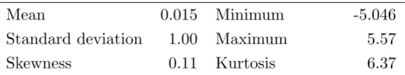
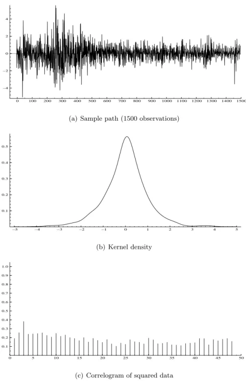
We use the S&P500 daily percentage returns from 19/07/2001 to 20/04/2007 (1500 obser-vations) for estimation. Figure 4 displays the sample path, the kernel density, and the cor-relogram of the squared returns. We observe a strong persistence in the squared returns, a slightly positive skewness, and a usual excess kurtosis for this type of data and sample size, see also Table 3.
Table 3: Descriptive statistics for S&P500 daily returns
Mean 0.015 Minimum -5.046
Standard deviation 1.00 Maximum 5.57
Skewness 0.11 Kurtosis 6.37
Sample period: 19/07/2001 to 20/04/2007 (1500 observations)
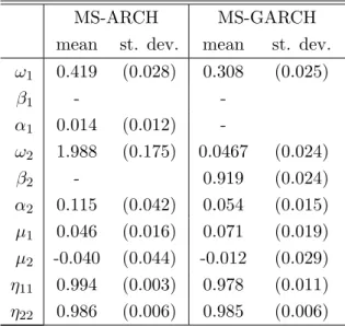
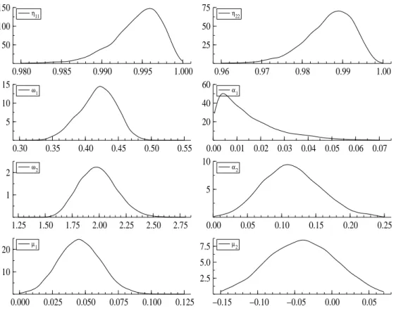
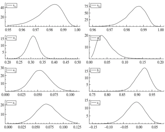
In Table 4, we report the posterior means and standard deviations from the estimation of different models using the estimation sample. The estimated models include the two-regime MS-ARCH model defined by setting β1 = β2= 0 in equations (3)-(4), and a restricted version (β1 = α1 = 0) of the corresponding MS-GARCH model. The marginal posterior densities
for these models are shown in Figures 5 and 6. The intervals over which the densities are drawn are the prior intervals (except for the transition probabilities). The intervals for the
0 100 200 300 400 500 600 700 800 900 1000 1100 1200 1300 1400 1500 −4 −2 0 2 4
(a) Sample path (1500 observations)
−5 −4 −3 −2 −1 0 1 2 3 4 5 0.1 0.2 0.3 0.4 0.5 (b) Kernel density 0 5 10 15 20 25 30 35 40 45 50 0.1 0.2 0.3 0.4 0.5 0.6 0.7 0.8 0.9 1.0
(c) Correlogram of squared data
Table 4: Posterior means and standard deviations (S&P500 daily returns)
MS-ARCH MS-GARCH
mean st. dev. mean st. dev. ω1 0.419 (0.028) 0.308 (0.025) β1 - -α1 0.014 (0.012) -ω2 1.988 (0.175) 0.0467 (0.024) β2 - 0.919 (0.024) α2 0.115 (0.042) 0.054 (0.015) µ1 0.046 (0.016) 0.071 (0.019) µ2 -0.040 (0.044) -0.012 (0.029) η11 0.994 (0.003) 0.978 (0.011) η22 0.986 (0.006) 0.985 (0.006) Sample period: 19/07/2001 to 20/04/2007 (1500 observations). A - symbol means that the param-eter was set to 0.
GARCH parameters were chosen to avoid negative values, and by trial and error so as to avoid truncation. The Gibbs sample size was fixed to 50,000 observations with a warm-up sample of 20,000, like for the simulation example.
When estimating the MS-ARCH model, we find that in the first regime, which is charac-terized by a low volatility level (ω1/(1 − α1) = 0.42 using the posterior means as estimates,
as opposed to 2.24 in the second regime), the ARCH coefficient α1 is close to 0 (posterior
mean 0.014, standard deviation 0.012, see also the marginal density in Figure 5). This is a weak evidence in favor of a dynamical effect in the low volatility regime. The same con-clusion emerges after estimating the MS-GARCH model, with the added complication that the β1 coefficient is poorly identified (since α1 is almost null). Thus we opted to report the
MS-GARCH results with α1 and β1 set equal to 0, and GARCH dynamics only in the high volatility regime. These results show clearly that the lagged conditional variance should be included in the second regime. Thus, the MS-ARCH model is not capturing enough the persistence of the conditional variance in the second regime. The second regime in the MS-GARCH model is rather strongly persistent but stable, with the posterior mean of β2 + α2 equal to 0.973 (0.919 + 0.054). If we estimate a single regime GARCH model, we find that
the persistence is 0.990 (0.942 + 0.048), which makes it closer to integrated GARCH than the second regime of the MS model. The estimation results for the MS-GARCH model also imply that compared to the first regime (where ω1 = 0.31), the second regime is a high volatility
regime since ω2/(1 − α2− β2) = 1.73. 0.980 0.985 0.990 0.995 1.000 50 100 150 η 11 0.96 0.97 0.98 0.99 1.00 25 50 75 η 22 0.30 0.35 0.40 0.45 0.50 0.55 5 10 15 ω 1 0.00 0.01 0.02 0.03 0.04 0.05 0.06 0.07 20 40 60 α 1 1.25 1.50 1.75 2.00 2.25 2.50 2.75 1 2 ω2 0.00 0.05 0.10 0.15 0.20 0.25 5 10 α 2 0.000 0.025 0.050 0.075 0.100 0.125 10 20 µ1 −0.15 −0.10 −0.05 0.00 0.05 2.5 5.0 7.5 µ2
Figure 5: Posterior densities for the MS-ARCH model (S&P500 daily returns)
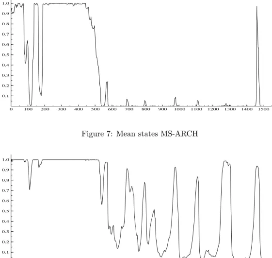
Another way to compare the two models is through the means of the state variables. These are obtained by averaging the Gibbs draws of the states. These means are smoothed (posterior) probabilities of the states. A mean state close to 1 corresponds to a high probabil-ity to be in the second regime. Figures 7 and 8 display the paths of these means. Both figures show, in conjunction with the sample path of the data (in Figure 4), that high probabilities are associated with high volatility periods (observations 1 to 500 and some peaks later). In this respect, the MS-ARCH model seems too insensitive in comparison with the GARCH version. From the posterior means of the MS-GARCH model, we can also deduce that the unconditional probabilities of the regimes are respectively 0.59 (= (1 − η11)/(2 − η11− η22))
0.95 0.96 0.97 0.98 0.99 1.00 20 40 η11 0.96 0.97 0.98 0.99 1.00 25 50 75 η22 0.20 0.25 0.30 0.35 0.40 0.45 0.50 5 10 15 ω1 0.00 0.05 0.10 0.15 0.20 10 20 ω 2 0.000 0.025 0.050 0.075 0.100 10 20 30 α 2 0.75 0.80 0.85 0.90 0.95 5 10 15 β2 0.000 0.025 0.050 0.075 0.100 0.125 10 20 µ1 −0.15 −0.10 −0.05 0.00 0.05 5 10 15 µ 2
Figure 6: Posterior densities for the MS-GARCH model (S&P500 daily returns) for the first one and 0.41 for the second one. These proportions correspond roughly to the information provided by the mean states.
5
Conclusion
We establish some theoretical properties for a Markov-switching univariate GARCH model with constant transition probabilities. We provide simple sufficient conditions for the er-godic stationarity of the process and the existence of its moments. We develop a reliable Bayesian estimation algortihm for this model, since ML estimation in not feasible due to path dependence.
Further research could be oriented in several directions. A first one consists in refining the specification by using existing extensions of the simple Gaussian GARCH model. A second direction of research is to specify the transition probabilities as a function of past information
0 100 200 300 400 500 600 700 800 900 1000 1100 1200 1300 1400 1500 0.1 0.2 0.3 0.4 0.5 0.6 0.7 0.8 0.9 1.0
Figure 7: Mean states MS-ARCH
0 100 200 300 400 500 600 700 800 900 1000 1100 1200 1300 1400 1500 0.1 0.2 0.3 0.4 0.5 0.6 0.7 0.8 0.9 1.0
Figure 8: Mean states MS-GARCH
as in Gray (1996). These extensions would render the algorithm more CPU-time consuming (due to the additional parameters) but would not complicate it fundamentally. Establishing the ergodic stationarity and existence of moments of such more richly specified processes would require to extend and adapt the proofs presented in the current paper. Finally further research could be focussed on estimating the model with other data series, and on comparisons with other GARCH models, in a similar way as done by Marcucci (2005).
Appendix
To prove Theorems 1 and 2, we write the model in its Markovian state space representation. We use the notation σ2
t = ht−1 to make it clear that σtis a function of the information dated
at time t − 1 or earlier, not information dated at t. Let λ and v denote the Lebesgue and the counting measures, respectively.
Proof of Theorem 1: There exists a measurable function g : S × < → S such that st = g(st−1, ξt), where the error term ξt is i.i.d. independent of ut and h0. Let ηt = (ut, ξt)0
and Zt is defined on D ⊂ < × <+× < where <+= (0, +∞). From (3) and (4), we have
Zt= yt ht st = µg(st−1,ξt)+pht−1ut ωg(st−1,ξt)+ αg(st−1,ξt)ε2 t + βg(st−1,ξt)ht−1 g(st−1, ξt) (15) = µg(st−1,ξt)+pht−1ut ωg(st−1,ξt)+ (αg(st−1,ξt)u2 t + βg(st−1,ξt))ht−1 g(st−1, ξt) = F (Zt−1, ηt) where F : D × <2 → D. Since η
t is independent of Zt−1 its follows from (15) that (yt, ht, st)0
forms a homogeneous Markov chain.
The process is defined on (D, =, ϕ). The state space of the process is given by D = {(y, h, s) ∈ < × <+× < : (y, h) ∈
Sn
i=1Di, s ∈ S}, where Di is the domain of the chain
in each regime and is given by Di = {(y, h) ∈ < × <+ : h ≥ ωi + αi(y − µi)2 + βi¯h} and
¯h = minβi<1{ωi/(1 − βi)} (see Zhang, Russell, and Tsay (2001)). The strict stationarity of
the first regime (E log(α1u2t + β1) < 0), implies that β1 < 1 (see, Nelson (1990)), hence ¯h
is well defined. The state space is equipped with =, the Borel σ−algebra on < × <+× <
restricted to D. The measure ϕ is the product measure λ2⊗ v on (D, =). We use Pm(z
0, A) =
P(Zt∈ A|Zt−m= z0) to signify the probability that (yt, ht, st) moves from (y0, h0, s0) to the
set A ∈ = in m steps.
In order to establish the geometric ergodicity of the Markov chain, we first show that the process is ϕ−irreducible. For irreducibility, it is sufficient to show that Pk(z
some k ≥ 1, for all z0 ∈ D and any Borel measurable sets A ∈ = with positive ϕ measure (see
Chan (1993)). We can show that from any (y0, h0, s0) ∈ D, all (y, h, s) ∈ A can be reached
in a finite number of steps. We assume that s0 = i, s = ` and ¯h is achieved in regime q.
Let ˜h = [h − ω`− α`(y − µ`)2]/β` and ς = ˜h − ¯h; since ˜h > ¯h we have ς > 0. Thus, there
exists a positive integer m = min(t ≥ 1 : ¯h + 0.5ς + 0.5β−t
q ς > ω1+ β1h0}, such that the point
(y, h, s) can be reached through the following m + 1 intermediate steps: w = {(yt, ht, st)}m+1t=1
where s1 = 1, st = q, ht = ¯h + 0.5ς + 0.5βqi−(m+1)ς, y1 = µ1 + [(h1 − ω1− β1h0)/α1]0.5,
yt= µq+ [0.5ς(1 − βq)/αq]0.5 for t ≤ m + 1 and in the m + 2-th step (y
m+1, ˜h, q) → (y, h, `).
The m+2-th step transition probability is absolutely continuous with respect to the ϕ measure. Thus, Pm+2(z
0, A) =
R
Apm+2(z0, z)dϕ(z), and by assumptions A1 and A2,
pm+2(z0, z) ≥
m+1Y i=0
f ((yi+1− µsi+1)/h0.5i )P(si+1|si) > 0,
which implies that Pm+2(z
0, A) > 0 and hence the chain is ϕ−irreducible. If z0 ∈ C, a
compact set, inf(z0,z)∈C×C pm+2(z
0, z) > δ > 0 and for any A ∈ = and z0 ∈ C,
Pm+2(z0, A) ≥ Pm+2(z0, A ∩ C) ≥
Z
A∩C
pm+2(z0, z)dϕ(z) ≥ δϕ(A ∩ C).
Therefore, P(z0, A) is minorized by ϕ(· ∩ C) which implies that all non-null, compact sets in
D are small by definition, see Meyn and Tweedie (1993, p. 111), and can serve as test sets. Using the same arguments as above, we can show that any small set can be reached in m + 3 steps, therefore the chain is aperiodic, see Chan (1993).
From (4) and the cr inequality we get
h1/tt ≤ [ωst + (αstu2t + βst)ht−1]1/t (16) ≤ (ωst)1/t+ (αstut2+ βst)1/t(ωst−1)1/t+ [(αstu2t + βst)(αst−1u2t−1+ βst−1)]1/th 1/t t−2 .. . ≤ t Y j=1 (αsju 2 j + βsj) 1/th+ t−1 X j=0 (ωst−j−1) 1/t j Y i=0 (αst−iu 2 t+ βst−i) 1/t+ (ω st)1/t
Since {st} is an ergodic Markov chain, for any initial state, we have that
1 t t X j=1 log(αsju 2 j + βsj) → n X i=1 πiE[log(αiu2t+ βi)] < 0, a.s. (17)
see Chan (1993). This result, with assumption A1 and the dominated convergence theorem imply that there exists a ¯t sufficiently large such that δ ≥ 1/¯t = p and for all j ∈ S,
E t Y j=1 (αsju 2 j + βsj) p|s 0 = j = γ < 1. (18)
As a drift function we use V (z) = 1 + (¯η/∆)y2p + hp, where ¯η = η − γ, ∆ = E(u2p
t ),
p = 1/¯t and η is some positive number which satisfies γ < η < 1 and the test set is given by C = {(y, h, s) ∈ D : h + y2≤ c, s ∈ S}, where c > 0 is to be determined below.
From (16)-(18), we find E(hpt|z0= z) ≤ 1 + E t Y j=1 (αsju 2 j + βsj) p|s 0= j hp+ M ≤ M + γhp where M = 1 + E Ã t−1P j=0 (ωst−j−1)p j Q i=0 (αst−iu2t + βst−i)p+ (ωst)p|s0 = j ! and M < ∞ by as-sumption A1. Therefore,
E(V (zt)|z0 = z) ≤ 1 + M + γhp+ ¯ηE(hpt|z0= z)E|u2pt |)/∆ ≤ hp µ
M hp + η
Since the Lyapounov function above is bounded on compact sets and h < V (z), we can choose c and η0 ∈ (η, 1) such that E( V (z
t)|z0= z) ≤ η0· V (z) + a · 1C(z) for some a < ∞ and for all
z ∈ D, hence the drift criterion is satisfied. We can then combine Meyn and Tweedie (1993, Theorem 15.0.1) and Tjostheim (1990) to obtain that {Zt} is geometrically ergodic and so
is {yt}. The finiteness of E(|Zt|p) with respect to the stationary measure follows from Meitz
and Saikkonen (2006, Lemma 6). If the process is initiated from its stationary distribution, it further follows that the process is β-mixing with geometrically decaying mixing numbers, see Doukhan (1994, p.89).
Proof of Theorem 2: Let Ij be an 1 × n matrix that contain 1 on the j-th position
and zeros elsewhere and l = (1, . . . , 1) be an n × 1 vector. The matrix Ω is positive, hence the spectral radius is real and positive and assumption A5 implies that there exists a positive integer r such that each element of Ωris smaller than1/n, that is (Ωr)ij < 1/n, see Lutkepohl
(1996, p. 76, 3(a)), hence E Yr j=1 (αsju2j + βsj)h |Z0 = (y, h, j) = (IjΩ)Ωr−1lh = γ < 1.
By solving (4) recursively and setting h0 = h, we get ht= [ωst + (αstu2t + βst)ht−1] = r Y j=1 (αsju2j + βsj)h+ r−1 X j=0 ωst−j−1 j Y i=0 (αst−iu2t + βst−i) + ωst. (19) Let ∆ = E(u2kt ) and ¯η = η − γk where η is some positive number which satisfies γk< η < 1. We select a drift function of the form V (y, h, s) = 1 + (¯η/∆)y2k + hk and a test set C =
{(y, h, s) ∈ D : h + y2 ≤ c, s ∈ S}. By the binomial theorem, (19), assumption A4 and some tedious calculations, we find
E(V (yt, ht)|Z0 = (y, h, j)) = 1 + E(ht|z) + ¯ηE(yt2k|z)/∆ =
1 + E Yr j=1 (αsju2j + βsj)j k
hk+ ¯ηhk+ o(hk) ≤ hk(γk+ ¯η + o(1)) ≤ hk(η + o(1)) By applying the same arguments as in Theorem 1, the desired result follows.
References
Abramson, A., and I. Cohen (2007): “On the stationarity of Markov-switching GARCH processes,” Econometric Theory, 23, 485–500.
Bauwens, L., A. Preminger, and J. Rombouts (2006): “Regime switching GARCH models,” CORE DP 2000/11, Universit´e catholique de Louvain, Louvain La Neuve. Bollen, S., N. Gray, and R. Whaley (2000): “Regime-Switching in Foreign Exchange
Rates: Evidence From Currency Option Prices,” Journal of Econometrics, 94, 239–276. Bollerslev, T., R. Engle, and D. Nelson (1994): “ARCH Models,” in Handbook of
Econometrics, ed. by R. Engle, andD. McFadden, chap. 4, pp. 2959–3038. North Holland Press, Amsterdam.
Cai, J. (1994): “Markov Model of Unconditional Variance in ARCH,” Journal of Business and Economics Statistics, 12, 309–316.
Chan, K. (1993): A Review of Some Limit Theorems of Markov Chains and Their Applica-tions. In H.Tong, Editor, Dimension Estimation and Models, World Scientific Publishing, Singapore and River Edge, NJ, USA.
Das, D., and B. H. Yoo (2004): “A Bayesian MCMC algorithm for Markov switching GARCH models,” Manuscript, City UNiversity of New York and Rutgers University. Diebold, F. (1986): “Comment on Modeling the Persistence of Conditional Variances,”
Econometric Reviews, 5, 51–56.
Doukhan, P. (1993): Mixing: Properties and Examples. Springer-Verlag, New-York.
Dueker, M. (1997): “Markov Switching in GARCH Processes in Mean Reverting Stock Market Volatility,” Journal of Business and Economics Statistics, 15, 26–34.
Francq, C., M. Roussignol,andJ.-M. Zakoian (2001): “Conditional heteroskedasticity driven by hidden Markov chains,” Journal of Time Series Analysis, 22, 197–220.
Francq, C., and J.-M. Zakoian (2002): “Comments on the paper by Minxian Yang: ”Some properties of vector autoregressive processes with Markov-switching coefficients”,” Econometric Theory, 18, 815–818.
(2005): “The L2-structures of standard and switching-regime GARCH models,” Stochastic Processes and their Applications, 1158, 1557–1582.
Gray, S. (1996): “Modeling the conditional distribution of interest rates as a regime-switching process,” Journal of Financial Economics, 42, 27–62.
Haas, M., S. Mittnik,andM. Paolella (2004): “A New Approach to Markov-Switching GARCH Models,” Journal of Financial Econometrics, 2, 493–530.
Hamilton, J.,and R. Susmel (1994): “Autoregressive Conditional Heteroskedasticity and Changes in Regime,” Journal of Econometrics, 64, 307–333.
Henneke, J. S., S. T. Rachev, and F. J. Fabozzi (2006): “MCMC based estimation of Markov Switching ARMA-GARCH models,” Working Paper, University of Karlsruhe. Kaufman, S., and S. Fruhwirth-Schnatter (2002): “Bayesian analysis of switching
ARCH models,” Journal of Time Series Analysis, 23, 425–458.
Kaufman, S.,andM. Scheicher (2006): “A switching ARCH model for the German DAX index,” Studies in Nonlinear Dynamics and Econometrics, 10/4, Article 3.
Klaassen, F. (2002): “Improving GARCH Volatility Forecasts with Regime-Switching GARCH,” Empirical Economics, 27, 363–394.
Lamoureux, C., and W. Lastrapes (1990): “Heteroskedasticity in Stock Return Data: Volume versus GARCH Effects,” Journal of Finance, 45, 221–229.
Lutkepohl, H. (1996): Handbook of Matrices. Wiley, New-York.
Marcucci, J. (2005): “Forecasting stock market volatility with regime-switching GARCH models,” Studies in Nonlinear Dynamics and Econometrics, 9, 1–53.
Meitz, M., and P. Saikkonen (2006): “Stability of nonlinear AR-GARCH models,” SSE/SFI Working paper series in Economics and Finance No. 632.
Meyn, S., and R. Tweedie (1993): “Markov Chains and Stochastic Stability,” London, Springer Verlag.
Mikosch, T., and C. Starica (2004): “Nonstationarities in Financial Time Series, the Long-Range Dependence, and the IGARCH Effects,” Review of Economics and Statistics, 86, 378–390.
Nelson, D. B. (1990): “Stationarity and Persistence in the GARCH(1,1) Model,” Econo-metric Theory, 6, 318–334.
Schwert, G. (1989): “Why Does Stock Market Volatility Change Over Time?,” Journal of Finance, 44, 1115–1153.
Tanner, M., and W. Wong (1987): “The Calculation of the Posterior Distributions by Data Augmentation,” Journal of the American Statistical Association, 82, 528–540. Tjostheim, D. (1990): “Non-linear time series and Markov chains,” Advances in Applied
Probability, 22, 587–611.
Yang, M. (2000): “Some properties of vector autoregressive processes with Markov-switching coefficients,” Econometric Theory, 16, 23–43.
Yao, J. (2001): “On square-integrability of an AR process with Markov switching,” Statistics and Probability Letters, 52, 265–270.
Yao, J., and J.-G. Attali (2000): “On stability of nonlinear AR process with Markov switching,” Advances in Applied Probability, 32, 394–407.
Zhang, M. Y., J. Russell, and R. Tsay (2001): “A nonlinear autoregressive conditional duration model with applications to financial transaction data,” Journal of Econometrics, 104, 179–207.