an author's https://oatao.univ-toulouse.fr/24323
https://doi.org/10.1145/3356401.3356412
Daigmorte, Hugo and Boyer, Marc Impact on credit freeze before gate closing in CBS and GCL integration into TSN. (2019) In: 27th International Conference on Real-Time Networks and Systems (RTNS 2019), 6 November 2019 - 8 November 2019 (Toulouse, France).
Impact on credit freeze before gate closing in CBS and GCL
integration into TSN
Marc Boyer
ONERA/DTIS, University of Toulouse F-31055 Toulouse, France
Hugo Daigmorte
ISAE-SUPAERO, University of Toulouse Toulouse, France
ABSTRACT
The Time Sensitive Networking (TSN) task group has added a set of mechanisms to Ethernet in order to provide a real-time network. In particular, the output port scheduling based on a Credit-Based Shaper (CBS) algorithm, that was introduced formerly by the Audio-Video Bridging (AVB) task group, has been enhanced with a time driven Gate Control List (GCL). This implies some update in the credit evolution rules, and several solutions may exist. In this paper, we compare the solution used in the standard with another one used in most papers, and also with a third one, designed as a trade-off between the two others. The comparison is first done on some hand-made examples, showing some credit overflow and unfairness potential problems. Then, simulations are done on a single switch with 3 CBS queues.
ACM Reference Format:
Marc Boyer and Hugo Daigmorte. 2019. Impact on credit freeze before gate closing in CBS and GCL integration into TSN. In 27th International Conference on Real-Time Networks and Systems (RTNS 2019), November 6–8, 2019, Toulouse, France. ACM, New York, NY, USA, 10 pages. https://doi.org/ 10.1145/3356401.3356412
1
INTRODUCTION
In order to offer real-time guarantees to audio and video flows over Ethernet, the Audio-Video Bridging (AVB) task group has defined a set of extensions of the IEEE 802.1Q standard [1], related to the forwarding policy in bridges (aka. switches). Among the 8 queues, the two with higher priority (called A and B) are scheduled at the output port of each switch with a specific policy, the Credit-Based
Shaper (CBS). At configuration, each queueX ∈ {A, B} receives
a part of the output port rateR, called the “idle slope”. Then, a
scheduler based on a credit variable implements this constraint (this algorithm will be described in Section 2.2).
Thereafter the Time Sensitive Networking (TSN) task group has added new extensions. One of them, named “Enhancement for scheduled traffic”, introduced per queue gates: each queue has access to the output port only when its gate is open, and the open-ing/closing of the gates is controlled by a cyclic time based schedule, called Gate Control List (GCL). The introduction of this mechanism
is interpreted by some authors as the introduction of Scheduled Traffic or Time-Triggered communications in TSN [3]. The CBS al-gorithm has been adapted to take into account the GCL mechanism. There are several ways to do such an adaptation and, surprisingly, the choice made in the standard is different from what is considered in the literature.
This paper will first present in Section 2 the sub-part of the TSN standard that is considered in this paper. Section 3 gives an overview of the assumptions done in the literature. Then, for some examples, the qualitative impacts of these new rules will be discussed in Section 4: the transformation of the operator slope into the credit idle slope, the possible credit overflow and some unfairness between flows w.r.t. AVB behaviour. After these preliminary considerations, Section 5 will formally define in an unified framework the standard evolution rule, the one assumed by most research papers, and a new one, a trade-off inspired by AVB. These three rules are compared by simulating a single output port with three CBS queues in Section 6. For sake of simplicity, this paper does not address preemption.
2
OUTPUT PORT MODEL
This section presents the sub-part of the 802.1Q standard [1] rel-evant for this study. Subsection 2.1 presents the global standard architecture, subsection 2.2 presents the credit based shaper rules defined before the introduction of gates, subsection 2.3 presents the evolution of those rules due to the introduction of gates, and subsection 2.4 presents some hypotheses limiting the scope of this study.
2.1
Output port architecture
In the current 802.1Q standard [1], a TSN output port is made of (up to) 8 queues, numbered from 0 to 7. To each queue is associated an optional transmission selection algorithm, and a gate that can be either open (o) or closed (c) as illustrated in Figure 1. A frame in a queue can be selected for transmission only if the transmission selection algorithm allows it (subsection 2.2 presents the credit based shaper, CBS, selection algorithm) and if the gate is open. A static global cyclic table, the GCL, schedules the gate openings and closings. If several frames are ready for transmission, the higher priority queue is selected (the higher the queue id, the higher the priority). Each frame is mapped into a class, and each class into a queue. In this paper, we will assume one queue per class, and use queue and class as synonyms.
2.2
Credit evolution rules without GCL
The Credit-Based Shaper (CBS, [1, §8.6.8.2]) is one possible trans-mission selection algorithm. This section presents the selection rules of CBS, when no GCL is implemented in the output port.
SP Transmission
selection
algorithms Gate Control List
? o|c ? o|c ? o|c ? o|c ? o|c ? o|c ? o|c ? o|c 7 6 5 4 3 2 1 0
Figure 1: TSN outputput port architecture
These selection rules rely, for each CBS queueX , on the value
of an integer variable, called credit and a parameter, idX, the idle
slope. The rules, when no GCL is used, are the following: R1: The head of queue frame can be selected for transmission only
if the credit of this queue is non negative, and no higher priority frame is ready for transmission.
R2: During frame transmission, the credit decreases as a function
of time with “send slope” rate sdX = idX−R where R is the
transmission rate of the port.
R3: The credit increases with rate idX when either the credit is
negative, or it is positive and there is some frame waiting in the queue.
R4: If the credit is positive and the queue is empty, the credit is reset to null.
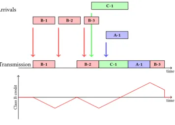
This behaviour is illustrated on an example with three active classes: A, B, and C, with A having the highest priority and C the lowest. Figure 2 shows the arrivals of frames (the frame X-n being
then-th frame entering queue X), the port transmission schedule
and the credit of class B (with null initial value). When a message
B-1is set in the queue, the credit is null, and from rule R1, it can
be selected for transmission. Then, rule R2 implies that the credit decreases. When message B-2 is received, it can not be selected since the credit is negative, and it must wait until the credit of class B reaches 0 to be selected. At the end of B-2 transmission, the output port is idle, and a lower priority message C-1 can start its transmission. Since we do not consider preemption, when the credit of class B reaches 0, the message can not be send, and the credit still increases, reaching positive values. However at the end of C-1 transmission, a higher priority frame A-1 is waiting, and B-3 has to wait. Thus its credit still increases. Finally message B-3 is selected for transmission, rule R2 implies that the credit decreases. At the end of B-3 transmission, the credit is positive and the queue is empty so, from rule R4, the credit is reset to null.
2.3
Credit evolution rules with GCL
The introduction of gates in [1, §8.6.8.4] comes with a modification of credit evolution rules. The main ideas are:
time time Class B cr edit Transmission Arrivals C-1 C-1 B-1 B-2 B-3 B-1 B-2 B-3 A-1 A-1
Figure 2: CBS credit evolution rules (without GCL)
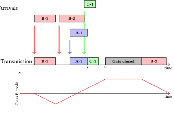
R5: The credit is frozen when the gate is closed (overriding rules R2 and R3).
R6: A frame can start its transmission if it can be sent up to com-pletion before the next gate-close event.
Moreover, the idle slope is scaled proportionally to the accumulated closing duration (more details will be given in Section 4).
This new behaviour is illustrated in Figure 3. Moreover the GCL list is in this example such that, when the gate of a queue is open, all other gates are open, and when the gate of a queue is closed, all other gates are closed. When message B-1 is set in the queue, the credit is null, and from rule R1, it can be selected for transmission. Then, rule R2 implies that the credit decreases. When message B-2 is received, it can not be selected since the credit is negative, and it must wait until the credit of class B reaches 0 to be selected. When message A-1 is received, the output port is idle, it can be selected for transmission. When the credit of class B reaches 0, the message can not be sent (the output port is used by frame A-1), the credit still increases, reaching positive values. The gate closing influence
starts at the end of A-1 transmission (time instants): rule R6 implies
that message B-2 has to wait. However a lower priority message
C-1can start its transmission. When the gate is closed, from rule
R5, the credit of class B is frozen. When the gate opens, message
B-2can start its transmission. At the end of B-2 transmission, the
credit is positive and the queue is empty so, from rule R4, the credit is reset to null.
One point deserves some attention: what happens just before gate closing? The rule R6 prevents a frame to encroach on a closed gate period: a frame can not start its transmission if it does not
have enough time to finish before the next gate-close event1. A
time interval when a frame can not start its transmission due to rule R6 will be called a “pre-closing” time interval. But what is the evolution rule of the credit during this time? In previous studies [10, 16], this period has been considered as an “extension” of the gate closing period, and it was assumed that the credit was also frozen. But in the current standard [1], the credit increases during
1The use of preemption may reduce this “forbidden” time, but it can not completely
Impact on credit freeze before gate closing in CBS and GCL integration into TSN RTNS 2019, November 6–8, 2019, Toulouse, France time time Class B cr edit Transmission Arrivals C-1 C-1 B-1 B-2 B-1 B-2 A-1 s A-1 u Gate closed
Figure 3: CBS credit evolution rules (with GCL)
this waiting time2. This paper focuses on the effect of these rules
on the port traffic scheduling.
2.4
Port with CBS and exclusive gating
This paper focuses on the interactions between the GCL and CBS mechanisms. It will then restrict the experiments on a specific class, where
• all queues except the highest and lowest priority (the ones with respective indexes 7 and 0) ones have a CBS shaper as the transmission selection algorithm,
• the highest and lowest priority queues have no transmission selection algorithm,
• the GCL list is such that, when the gate of the highest priority queue (the one with index 7) is open, all other gates are closed, and when the gate of the highest priority queue is closed, all other gates are open (aka. exclusive gating). To ease comparison with AVB, CBS queues will be named A,B,C,D,E,F, as illustrated on Figure 4.
3
STATE OF THE ART
Scheduling synchronous and asynchronous workload on a given resource is an old issue. For example, the “deferrable server” [15] considers a set of strictly periodic tasks, plus a deferrable server, designed to execute the asynchronous workload. Like CBS, this server receives periodically a capacity, a credit, of execution time. But a deferrable server can use all its credit to execute several pending asynchronous tasks, whereas the replenishment rules of CBS are designed to limit such bursts (as illustrated by the delaying of frame B-2 in Figure 2). Moreover, deferrable server assumes preemptive scheduling, whereas the core is this paper is the impact that non-preemption and encroaching avoidance have on credit.
More recently, another Ethernet-based solution mixing synchro-nous (Time-Triggered) and asynchrosynchro-nous (Rate Constrained) flows has been developed: TTEthernet [14]. Three integration policies
2A detailed analysis of this sub-part of the standard devoted to CBS credit evolution
rules and GCL interactions can be found in [5].
SP Gate Control List
y CBS y CBS y CBS y CBS y CBS y CBS y x Highest priority / 7 A / 6 B / 5 C / 4 D / 3 E / 2 F / 1 Best effort / 0
Figure 4: TSN output port with High Priority / CBS / Best Effort and exclusive gating between High Priority queue and other queues. {x,y} = {o, c}
have been defined in [14] to solve (or limit) the encroaching of asyn-chronous flow on synasyn-chronous time windows. But this technology has no credit-based shaping mechanism.
There are, to the best of our knowledge, few studies discussing this specific point of credit evolution rule before gate-close event in the TSN context.
The first proposal on adding some time scheduled traffic to AVB seems to be done in [3], calling the proposal “AVB ST”. It shows that to avoid encroaching on reserved time windows, called “ST slots”, some “guard bands” have to be considered. The credit evolution rule is the one of AVB: when a CBS queue waits, its credit increases, whether this waiting is due to any guard band or a ST slot. A worst case response time AVB ST is done in [4], making clear distinction between the standard behaviour of TSN and the AVB ST proposal. All other papers, analysing TSN configurations with CBS and GCL mechanisms, either by simulation or evaluating the worst case latency, assume that there is a “guard band” before the gate-close event, and that during this guard band, the credit is frozen [7, 10, 10, 16].
Last, in [6], when looking for a worst case latency bound, sev-eral integration policies are considered, and a generic model that generalises all these policies is defined. It might be generic enough to be used with the standard rules.
4
IMPACT OF CREDIT EVOLUTION RULES
This evolution of credit before a gate-close event can have unex-pected consequences. The reason is that, for a given class, there are two sources of bandwidth loss due to gate closing: some is lost while the gate is closed, and during these intervals, the credit is frozen, whereas some is lost while the gate is open, and during these intervals, the credit increases.In this section, we will first show that the pre-closing time (this time when a frame can not be sent since there is not enough time to send a frame before the next gate-close event) can not be “used” by CBS flows: if this time is statically allocated to CBS flows, it can lead to buffer overflow (Section 4.2.1), and if it is not, it will lead to CBS idling time, whereas there is backlog and idle port
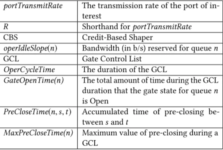
Table 1: Glossary
portTransmitRate The transmission rate of the port of
in-terest
R Shorthand for portTransmitRate
CBS Credit-Based Shaper
operIdleSlope(n) Bandwidth (in b/s) reserved for queuen
GCL Gate Control List
OperCycleTime The duration of the GCL
GateOpenTime(n) The total amount of time during the GCL
duration that the gate state for queuen
is Open
PreCloseTime(n, s, t) Accumulated time of pre-closing
be-tweens and t
MaxPreCloseTime(n) Maximum value of pre-closing during a
GCL
(Section 4.2.2). Second, we will show in Section 4.3 that these rules can be unfair: it allows the CBS queues with the highest priority to gain more credit, and send larger bursts than in a pure AVB system, creating larger jitter for low priority CBS queues. But before discussing the differences and interactions between these elements, some vocabulary has to be introduced.
4.1
Vocabulary
Let portTransmitRate be the transmission rate of the port of in-terest and let OperCycleTime be the duration of the GCL table
(the period of the behaviour). Letn ∈ [0, 7] be a queue number,
GateOpenTime(n) is the total amount of time during the GCL
du-ration that the gate state for queuen is open, GateCloseTime(n)def=
OperCycleTime−GateOpenTime(n), the total amount of time during
the GCL duration that the gate state for queuen is Closed. The
network designer has to set the operIdleSlope(n) of each queuen
using CBS, the bandwidth allocated to this queue [1, § 34.3]. All these values are statically defined. Now, given an interval [s, t], PreCloseTime(n, s, t) is the accumulated time where some frame has been delayed because of rule “there is insufficient time available to transmit the entirety of that frame before the next gate-close
event”3. This duration is by nature dynamic: it depends on the
pres-ence of frame in the queue before some gate-close event, on the credit value, and on the frame size. It can be upper bounded: each close-gate event may generate only one pre-close interval, and its length is at most the duration of one frame of maximal length. Let
MaxPreCloseTime be its maximal value on a GCL cycle4.
Then, the idleSlope parameter is computed as in [1, §8.6.8.2]
idleSlope(n) = operIdleSlope(n) × OperCycleTime
GateOpenTime(n) (1)
3We chose the term “pre-closing” time for these intervals, instead of “guard band”
which is more commonly used, because depending on the authors, the “guard band” is this dynamic pre-closing time, whereas for others, the “guard band” is a static interval before the gate-close event, whose length must be large enough to prevent any encroaching. In the standard itself, the term “guard band” is used only in an informative appendix [1, Appendix Q], and without any exact definition.
4The terms portTransmitRate, OperCycleTime, GateOpenTime operIdleSlope, are from
the standard, the terms GateCloseTime, PreCloseTime and MaxPreCloseTime have been introduced to ease the discussion.
0 500 1000 1500 2000 2500 3000 3500 4000 time (ms) 200 100 0 100 200 300 400 500 credit (b) A B Gate closed
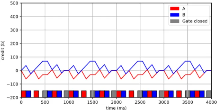
Figure 5: Credit overflow
whereOperCycleTimeGateOpenTime is the fraction of time the gate is open. Table 1
summarises all of this information.
4.2
The pre-closing time can not be used by
CBS flows
This section presents how the evolution rules of credit prevent the use of this pre-closing time by CBS flows: first, in Section 4.2.1, how the static configuration of parameters prevents from stati-cally reserving it for CBS flows, second, in Section 4.2.2, how the transmission rules prevents CBS flows from dynamically using it.
4.2.1 Pre-closing time can not be allocated to CBS flows. During
the configuration, the pre-closing time can not be allocated to CBS. Otherwise, the value of the credit is unbounded and its implemen-tation variable can overflow (in the remainder of this paper we will write “credit overflow” to speak about the credit implementation overflow).
Consider a TSN output port with CBS at queues 1 to 6 and
exclusive gating, as presented in Section 2.4. For any priorityn ∈
[1, 6], the condition Õ i ∈hp(n) operIdleSlope(i) R + GateCloseTime(n) OperCycleTime +MaxPreCloseTime(n) OperCycleTime ≤ 1 (2)
must hold, where hp(n) denotes the set of CBS queues with
prior-ity not smaller than thenth queue5. Otherwise, the credit of the
priority leveln can overflow. This condition just states that the
global load must be less than 1, consideringρi =operIdleSlope(i)R the
load associated to higher priority flowi, ρGCL = GateCloseTime(n)OperCycleTime
the load associated to GateCloseTime, and a “virtual” loadρPreC=
MaxPreCloseTime(n)
OperCycleTime associated to pre-closing.
An example of overflow is illustrated in Figure 5: in this example, there are two CBS flows, class A and class B. The evolution of their credits is represented at the top of the figures, as in subsequent figures. At the bottom of the figures, as in subsequent figures, is represented the transmission of the messages (A or B) as well as the gate state (grey when the gate is closed). The OperCycleTime is set
5Whereas it is common in real-time community to consider that the index 0 has the
highest priority, in the 802.1Q standard, the queue with index 0 has the lowest priority, and so, hp(n) = {n, n + 1, . . . , 6}.
Impact on credit freeze before gate closing in CBS and GCL integration into TSN RTNS 2019, November 6–8, 2019, Toulouse, France 0 500 1000 1500 2000 2500 3000 3500 4000 time (ms) 200 100 0 100 200 300 400 500 credit (b) A B Gate closed
Figure 6: Unused bandwidth
equal to 1000ms, the portTransmitRate is also 1b/ms, all messages are of constant sizes 100b and the GateCloseTime represents 20% of the OperCycleTime divided into two windows of duration 100ms (One may object that it is not possible to have Ethernet frames of size 100b, and that 1b/ms is unrealistic. But this example has been built to illustrate some behaviour with a small number of frames, human-friendly constants and can be scaled to realistic values). Both examples assume that the queues are never empty during the considered interval. In this example the sum of allocated bandwidth plus the GateCloseTime is equal to portTransmitRate (class A and class B operIdleSlope equal 400b/s). But since a part of the bandwidth allocated is in fact lost by pre-closing time, it leads to credit overflow.
4.2.2 Un-allocated time can not be used by CBS flows. The
previ-ous example has shown that the pre-closing time, which is by nature dynamic, can not be allocated to CBS flows. One may wonder if it can be dynamically used by these flows. Consider a second example (see Figure 6) with the same parameters as the previous one, except that the sum of allocated bandwidth plus the GateCloseTime plus the MaxPreCloseTime is equal to portTransmitRate (class A and class B operIdleSlope equal 300b/s). In this case, there is no more overflow; however there is some unused bandwidth. The reason is that the idle slope of a CBS queues acts both as a minimal reserved capacity, but also as a maximal bandwidth usage (it is both the slope of the minimal service curve and the shaping curve [12]). Then, since the MaxPreCloseTime has not been allocated to CBS flows (to avoid possible credit overflow), it can not be used by these CBS flow.
This behaviour is not surprising: whereas GPS-like policies (WFQ, WRR, DRR [9, 11, 13]) are designed to dynamically share the band-width in a fair way (with configurable weights between flows), credit based shaping reserves a constant capacity. In TSN, to avoid encroaching on static gate closing, some dynamic loss of bandwidth is created, and credit based shaping can not share it between flows (but it may be used by some Best-Effort queue, i.e. queue with low priority flows and without shaper).
4.3
The pre-closing time credit evolution rule
can be unfair
A more unexpected consequence of the credit evolution rule is that it can be unfair: it can allow high priority classes to accumulate more credit, and create larger bursts than what would happen
0 1000 2000 3000 4000 5000 6000 time (ms) 200 150 100 50 0 50 100 150 200 credit (b) A B C Gate closed
Figure 7: Three CBS flows
0 1000 2000 3000 4000 5000 6000 time 200 150 100 50 0 50 100 150 200 credit A B C Gate closed
Figure 8: Credits increase during the pre-closing time
0 1000 2000 3000 4000 5000 6000 time (ms) 200 150 100 50 0 50 100 150 200 credit (b) A B C Gate closed
Figure 9: Credits are frozen during the pre-closing time
without gate closing. It would then increase the worst waiting time of low priority frames.
In order to visualise this unfair behaviour we will use the orig-inal situation described in Figure 7. In these examples there are three CBS flows : class A, class B and class C. In this example the GateCloseTime is null and the portTransmitRate is 1b/ms. 30% of the OperCycleTime is allocated to class A (operIdleSlope equal 300b/s), 20% is allocated to class B (operIdleSlope equal 200b/s) and 20% is allocated to class C (operIdleSlope equal 200b/s). Messages of each class are of constant sizes : 150b for A and 100b for B and C. Figure 7 shows that there is an alternation in the transmission of messages between these three classes.
Now we will consider a different situation. The traffic of the class A is split: two thirds remains in the class A, and one third is
set to the highest priority queue. The highest priority queue gets an exclusive access to the medium through GCL mechanism, as described in Section 2.4. The operIdleSlope of the class A is decreased to 200b/s, its message size is decreased to 100b. The part sent to the higher priority queue is cut into smaller packets of size 50b, with a
schedule6given at the bottom of Figure 8. Then, the behaviour of
the system is represented in Figure 8: the first frame of the C queue is delayed by two frames from A and two frames from B. The long term service is the same (in both Figures 7 and 8, 12 frames of C are served), but the traffic is more bursty, due to gate closing, but also to the credit evolution rule.
Now we will consider that during the pre-closing time, the credit is frozen (like when the gate is closed). The Figure 9 represents the same system than in Figure 8, but with credit frozen during pre-closing time. In this situation there is a perfect alternation in the transmission of messages between the three classes. This situation is more fair. However the part of unused bandwidth increases: since the credits no longer increase during PreCloseTime, only 10 frames per class are served during this schedule. The reason is in the conversion between the operIdleSlope and the idleSlope: the eq. 1 does not consider the effect of pre-closing. This point will be discussed in Section 5.
5
DIFFERENT EVOLUTION RULES
In this section, we will formally define in an unified framework the standard evolution rule, the one assumed by most research papers, and a new one, a trade-off inspired by AVB. We will first take a look at some important CBS properties (Section 5.1) before discussing several possible credit evolution rules (Section 5.2).
5.1
Two framing remarks
Before discussing and comparing different rules for the credit evo-lution, let us make two framing remarks.
Keeping credit value bounded. First, one must avoid any credit overflow. We have shown in Section 4.2 that the pre-closing time can not be allocated to CBS flows. In other words, one can interpret the pre-closing time as the time where the link is used by a virtual higher priority flow. Since the operate idle slope operIdleSlope(i) of
a classi can be interpreted as a part of the bandwidth reserved for
this class, one must take into account the bandwidth used by the virtual flow, and the total bandwidth allocation must be less than the link capacity. That is to say, the equation 2 must hold. Note that, like for other CBS flows, the bandwidth that was reserved for this virtual “pre-closing” flow and that is not used is not lost since it may be used by best-effort flows.
AVB credit and bandwidth. Second, one should consider how the credit-based rule can ensure a throughput of idleSlope(X ) to a class X .
In AVB, when a classX starts at some time t to send a frame
of lengthL with null credit, it has to wait up to t + idL
X before
emitting a new frame, letting other flows send their frames. The credit goes up to positive values only when others AVB flows are
6Like in example of Figure 5, this example has been built to illustrate some behaviour
with human-friendly constants, leading to unrealistic Ethernet frames of size 50b, and a very non efficient schedule with very small intervals.
Link Class X cr edit time X-1 L1 L1 idX u v X-2 L2 L2 idX u′ v′
Figure 10: AVB credit evolution w.r.t. packet size;Li is the
size of packet X-i, idX the credit of class X.
Link Class X cr edit time X F sd X id X id X L I u v
Figure 11: Credit evolution rule and frozen time.
sending frames (or due to the non-preemption of one best-effort frame). That is to say, the credit can always increase and return back to zero when it has negative value, but it can increase to positive values only if another flow is using the link. Moreover, the amount of data sent in an interval [u,v] (where the credit ceases to be null at
u and comes back to 0 at v) is idX(v − u), as illustrated in Figure 10.
More generally, the credit mechanism offers a bandwidth idX to
class X (up to bounded credit variations). Let us now discuss several possible credit evolution rules.
5.2
Discussing new rules
Operator slope vs. idle slope. As presented in Section 5.1, the CBS mechanisms in AVB ensure that a class X with idle slope idX (expressed in bit per second), on any backlogged interval receives
at least idX, and can not use more than idX (up to the – bounded –
credit variation).
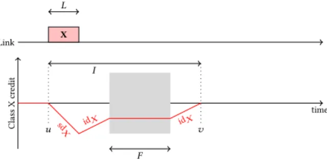
The integration of CBS and GCL has introduced some intervals
where the credit is frozen. Then, considering two instantsu, v
such that the credit ceases to be null atu and comes back to 0
atv, as illustrated in Figure 11. The quantity of data send is only
idX× (v −u − F (u,v)), where F (u,v) denote the credit freezing time
betweenu and v (in Figure 11, this is a single interval, but in the
general case, it may be the sum of several).
Considering the example of Figure 11, the relation between
L,u,v, F, idX isL = idX × (v − u − F ). Then, if the network
op-erator aims to offer to class X a bandwidth opX, one must set
idX = opX×v − u − Fv − u . (3)
In the current standard rule, this timeF (u,v) is statically known
Impact on credit freeze before gate closing in CBS and GCL integration into TSN RTNS 2019, November 6–8, 2019, Toulouse, France Arrivals Link Class X cr edit time gate closed X (S) (F) (R) Class X cr edit time gate closed X Y (S) (F) (R)
Figure 12: Possible credit evolution scenarios
offer a long-term bandwidth opX, on all a GCL schedule, starting
ats and ending at e, the idle slope is set as
idX = opX × e − s
e − s − F (s, e) =opX ×
OperCycleTime
GateOpenTime(X). (4)
But when considering a rule where this freezing time is dynamic,
one may only knowF, F such that F ≤ F (s, e) ≤ F , leading to two
possible definitions of the idle slope,
idX = opX × OperCycleTime
OperCycleTime −F (5)
or
idX = opX × OperCycleTime
OperCycleTime −F. (6)
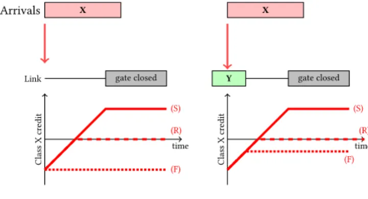
Credit evolution rule. Consider first the situation where a frame X is received while the credit of its class is negative (Figure 12, left part) and this frame is too large to be sent before the next gate-close event. The standard behaviour, labelled (S) considers that the credit increases up to gate-close event, and is frozen while the gate is closed. Previous studies assume that the credit is frozen is such case, leading to the dotted credit curve (F). But one may consider, by symmetry with AVB behaviour, that a negative credit can always increase and return to zero, but that a positive credit must be linked to a use of the link by another flow, leading to the dashed credit curve (R).
Considering several flows, more options appear, as presented in right part of Figure 12. While the frame X is blocked, it can exist another frame Y using the link. Moreover, it introduces another variation in the possible credit evolution rule: while Y is being sent, does the credit of X evolve or not? We chose in this study to let it increase, since it reduces the frozen time, which is a kind of “waste” of credit opportunity. Moreover, another class may have a head-of-queue frame Z small enough to be sent between Y and the gate-close event. In the current standard rules, this frame Z will be sent, and this appear to be a reasonable behaviour. But this highlights the fact that there is no “guard band” but a per-class behaviour, that we named “pre-closing”.
To formally define the rules (R) and (F), let us introduce two new boolean variables pre-closing, and closed. The boolean gate-closed is true when the gate is gate-closed, false otherwise. Definition of pre-closing depends on the policy and is postponed. In the cases of
AVB behaviour (R) and of frozen behaviour (F) the credit evolution rules are the following:
• the credit decreases during a frame transmission (which implies that the gate is open, i.e. gate-closed=False);
• the credit increases when gate-closed=False and pre-closing=False and
– either the credit is negative,
– or there is some frame waiting in the queue;
• the credit is frozen when gate-closed=True or pre-closing=True. It remains to define when pre-closing turns True and False. First pre-closing turns False when the gate closes. Second pre-closing turns True when the gate is open, the link is available (no message is being sent, and no high priority message can start its transmission) and
Return to zero (R): the credit is positive and the frame could not be sent up to completion before the next gate-close event. Frozen behaviour (F): the frame could not be sent up to
comple-tion before the next gate-close event.
Combining remarks on evolution rules and idle slope leads to 5 behaviours of interest: the standard one, denoted S, with the idle slope computed using eq. (4), the one freezing the credit when a frame can not be fully sent, denoted F, using either the idle slope id or id (resp. defined in eq. (5) and eq. (6)), and the negative values return to zero, denoted R, also with either id or id. But keep in mind
that using numerical values, id = id since the minimal freezing
time is the GateCloseTime.
6
EXPERIMENTS
This section evaluates the effects that credit evolution rules have on the traversal time of CBS messages. In order to evaluate these impacts, we first define an experimental configuration (Section 6.1). The results obtained are presented in Section 6.2 before being in-terpreted in the Section 6.3.
6.1
Simulation model and assumptions
In this paper, we decide to focus on a single node and a single transmit port. Then our configuration pattern is the following:
• The portTransmitRate is equal to 100 Mb/s.
• The architecture conforms to the hypotheses of Section 2.4: no transmission algorithm for higher and lower priority queues, CBS for all others, exclusive-gating between the higher priority queue and all others.
• Only 3 CBS queues are active (queue A, queue B and queue C):
– Their operIdleSlope are equal and set to 20 Mb/s. – The OperCycleTime is equal to 1s and the GateOpenTime
is equal to 0.8s.
– Each queue is shared by 20 stricly periodic flows with offsets and constant packet size.
– The period and size of each flow was uniformly chosen from the set {(1ms, 125bytes), (2ms, 250bytes), (4ms, 500bytes), (8ms, 100bytes)} so that the load of each flow is equal to 1 Mb/s.
• There is 1 BE flow in the lower priority queue, with messages of size randomly chosen between 125 bytes and 1250 bytes.
We consider two different configurations for the closing events of CBS and BE queues:
– Random: 1000 closed intervals, with duration of 0.2ms, are randomly set (without overlaping).
– Uniform: Every ms starts a closed interval (leading to 1000 closed interval), with a duration of 0.1ms, 0.2ms or 0.4ms randomly chosen, but such that there are 400 intervals of 0.1ms, 400 intervals of 0.2ms and 200 intervals of 0.4ms per OperCycleTime.
One simulation is done using this configuration pattern and by choosing randomly an offset for each flow. One simulation lasts 5 second and provides the delay for each message. In order to obtain representative results, statistics are done over 50 simulations,
leading to more than 5 × 10⁶messages. Now that we have our
configuration it is possible to compute the idle slopes defined in
equations (4) (5) and (6): id= 25Mb/s, id = 25 Mb/s and id = 27.78
Mb/s.
6.2
Results
As presented in Section 5, our aim is to evaluate 3 possible credit evolution rules, with different values of idle slope. In each case, 50 simulations have been run, each one with a different set of offsets between the (periodic) flows. The delays of each frame have been recorded during 5s of simulated time, and then grouped per class to get per class delay distribution. Since the delays depend strongly on the set of offsets, all the 50 delays distributions have been merged into a single one.
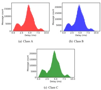
A first framing observation is that, for each experiment, the shapes of the three classes are similar: they may have different average or median values, but the shapes of the distributions curves look very similar, as shown on Figure 13. Then, next results plotting delay distribution will aggregate all classes into a single one, and the per class results will be given using box plots. The ends of the box are the lower and upper quartiles (Q1 and Q3) and the band inside the box is the median (Q2). The whiskers (the two lines outside the box) extend to the highest and lowest observations.
We then can compare the three policies, with the same value
of idle slope (id= id = 25Mb/s), first on the experiments with the
uniform gate closing (cf. Figure 14, and mind that the scales are different). Clearly, the frozen policy gives the worst results, and in fact, such a policy will lead to buffer overflow (but our simulator assumes infinite memory). The reason is that this policy, with this value of idle slope, does not offer enough throughput to the flows. In fact, it also is the case for the policy R considering the worst possible behaviours. But in this simulation, the credit has enough opportunities to get back to 0 before gate closing and avoid buffer overflow.
When considering a random allocation, (cf. Figure 15), the box plots are globally equivalent to the one of the uniform allocation, but the distributions of delay are different, as illustrated on Figure 16. This shows that the distribution of the gate closing instants has a significant impact on the delays, but this influence is out of the scope of this study.
The previous experiments have been done with the small value of the idle slope, id (25Mb/s in the experiment), which is insufficient for the policy R to serve all input flows, in theory, and insufficient
0.0 2.5 5.0 7.5 10.0 Delay (ms) 0 5000 10000 15000 Message count (a) Class A 0.0 2.5 5.0 7.5 10.0 Delay (ms) 0 5000 10000 15000 20000 Message count (b) Class B 0.0 2.5 5.0 7.5 10.0 Delay (ms) 0 5000 10000 15000 20000 Message count (c) Class C
Figure 13: Per class delay distribution for policy S, idle slope id, random gate closing.
in practice for the policy F. We may now have a look on the effect of a larger idle slope, id (27.78Mb/s in the experiment). In this set of experiments, we are going to set the idle slope of the S policy to 27.78Mb/s. This is not the value of the idle slope given by the standard, but comparing policy S with R and F, while giving S a smaller idle slope would have been an unfair comparison.
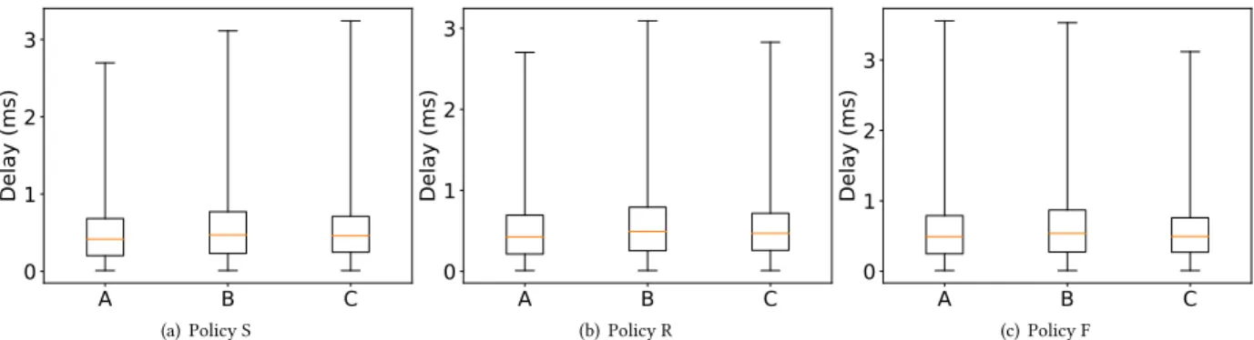
The delay distributions of all classes are plotted in Figure 17 and the per class box plots are given in Figure 18. When comparing the policies, it also appears that F is worse than the others, and that S and R have very similar results. But there is another important fact: while the idle slopes have been increased by only 11%, the average delays have been decreased by a factor of 8.
6.3
Discussing results
What can be learned from all these results? Mainly two things. First, freezing the credit of a class when it can not send any frame due to a gate closing (policy F) is not a very good solution with regard to the other solutions (policies S and R). Second, the delays do not increase linearly with the load with the standard mechanisms: when considering average delays, it is better to let the load be slightly smaller than the bandwidth allocated through the operator slope parameter. Last, the policy R, inspired by AVB, performs comparably to the standard mechanism.
7
CONCLUSION
This article pays attention to a small part of the TSN behaviour: the instants before a gate-close event, and their interactions with the CBS selection algorithm, and in particular the credit evolution rules before a gate-close event.
The starting point of this study is that several behaviours exist in the literature, without (up to our knowledge) any qualitative or quantitative comparison. In this paper, we have considered in a unified framework three policies: the one of the standard (denoted
Impact on credit freeze before gate closing in CBS and GCL integration into TSN RTNS 2019, November 6–8, 2019, Toulouse, France
A
B
C
0
2
4
6
8
Delay (ms)
(a) Policy SA
B
C
0
2
4
6
8
Delay (ms)
(b) Policy RA
B
C
0
50
100
150
Delay (ms)
(c) Policy FFigure 14: Box plot of delays (in ms), for policies S, R, and F, idle slope id= id, uniform gate closing.
A
B
C
0
2
4
6
8
10
Delay (ms)
(a) Policy SA
B
C
0
2
4
6
8
10
Delay (ms)
(b) Policy RA
B
C
0
50
100
150
Delay (ms)
(c) Policy FFigure 15: Box plot of delays (in ms), for policies S, R, and F, idle slope id= id, random gate closing.
0.0 2.5 5.0 7.5 Delay (ms) 0 10000 20000 30000 40000 Message count
(a) Uniform gate closing
0.0 2.5 5.0 7.5 10.0 Delay (ms) 0 20000 40000 60000 Message count
(b) Random gate closing
Figure 16: Delay distribution of all classes for policy S, idle slope id, uniform and random gate closing.
S), one that, as assumed in most of papers, freezes the credit before the gate closing (denoted F), and a third one, inspired by AVB, that allows the credit to return up to zero before a gate closing (denoted R). Whereas the differences can be considered as minor (just a few words to change in the standard), it has an impact. We have shown on some specific hand-made examples, presented in Section 4, that small modifications can lead to buffer overflow or unfairness be-tween classes. The impact on these variations have been evaluated by running 200 simulations for each of the three policies. It shows that it can have very significant impact on the performances. In particular, the policy F that is mainly considered in the literature, gives on simulation worse results than the standard behaviour S.
0 1 2 3 Delay (ms) 0 20000 40000 60000 80000 Message count (a) Policy S 0 1 2 3 Delay (ms) 0 20000 40000 60000 Message count (b) Policy R 0 1 2 3 Delay (ms) 0 20000 40000 60000 80000 Message count (c) Policy F
Figure 17: Delay distribution of all classes for policies S, R and F, idle slope id, uniform gate closing.
A
B
C
0
1
2
3
Delay (ms)
(a) Policy SA
B
C
0
1
2
3
Delay (ms)
(b) Policy RA
B
C
0
1
2
3
Delay (ms)
(c) Policy FFigure 18: Box plot of delays of all classes for policies S, R and F, idle slope id, uniform gate closing.
unfairness shown on examples has not been reproduced on these simulations.
This study must now be completed by some analysis on the worst case delays. The policy R has been designed to avoid too large values of the credit, which is a root of unfairness. The simulations have shown that it has mean performances equivalent to the standard, and one must investigate what are the differences on the worst case delays.
However, the preemption (presented in [2, 8]) will reduce the impact of gate closing on CBS flow, but it will not disappear. Without preemption, the maximum pre-closing is a full Ethernet frame (15KB), and with preemption, it will be reduced to a full fragment (1.6KB).
ACKNOWLEDGMENTS
We would like to thank Luxi Zhao from Technical University of Denmark for the valuables comments on a preliminary version of this paper.
REFERENCES
[1] 2018. IEEE Standard for Local and Metropolitan Area Networks – Bridges and Bridged Networks. IEEE Standard 802.1Q. IEEE.
[2] 802.1Qbu 2016. IEEE Standard for Local and metropolitan area networks – Bridges and Bridged Networks – Amendment 26: Frame Preemption. IEEE Standard 802.1Qbu. https://doi.org/10.1109/IEEESTD.2016.7553415
[3] Giuliana Alderisi, Gaetano Patti, and Lucia Lo Bello. 2013. Introducing support for scheduled traffic over IEEE audio video bridging networks. In Proc. of the 18th IEEE Conference on Emerging Technologies Factory Automation (ETFA 2013). 1–9. https://doi.org/10.1109/ETFA.2013.6647943
[4] Mohammad Ashjaei, Gaetano Patti, Moris Behnam, Thomas Nolte, Giuliana Alderisi, and Lucia Lo Bello. 2017. Schedulability analysis of Ethernet Audio Video Bridging networks with scheduled traffic support. Real-Time Systems 53, 4 (01 Jul 2017), 526–577. https://doi.org/10.1007/s11241-017-9268-5
[5] Hugo Daigmorte and Marc Boyer. 2018. Does the integration of CBS and GCL be-haves as you expect? And can it be enhanced? https://hal.archives-ouvertes.fr/hal-01961718. (Dec. 2018). working paper.
[6] Hugo Daigmorte, Marc Boyer, and Luxi Zhao. 2018. Modelling in network calculus a TSN architecture mixing Time-Triggered, Credit Based Shaper and Best-Effort queues. https://hal.archives-ouvertes.fr/hal-01814211. (June 2018).
[7] Feng He, Lin Zhao, and Ershuai Li. 2017. Impact Analysis of Flow Shaping in Ethernet-AVB/TSN and AFDX from Network Calculus and Simulation Perspec-tive. Sensors 17, 5 (2017). https://doi.org/10.3390/s17051181
[8] IEEE. 2016. IEEE Standard for Ethernet Amendment 5: Specification and Man-agement Parameters for Interspersing Express Traffic. IEEE Standard 802.3br. https://doi.org/10.1109/IEEESTD.2016.7900321
[9] Manolis Katevenis, Stefanos Sidiropoulos, and Costas Courcoubetis. 1991. Weighted round-robin cell multiplexing in a general-purpose ATM switch chip. Selected Areas in Communications, IEEE Journal on 9, 8 (1991), 1265–1279.
[10] Dorin Maxim and Ye-Qiong Song. 2017. Delay Analysis of AVB traffic in Time-Sensitive Networks (TSN). In RTNS 2017 - International Conference on Real-Time Networks and Systems. Grenoble, France, 10. https://doi.org/10.1145/3139258. 3139283
[11] Abhay K. Parekh and Robert G. Gallager. 1993. A generalized processor sharing approach to flow control in integrated services networks: the single-node case. IEEE/ACM Transactions on Networking (TON) 1, 3 (June 1993).
[12] Joan Adrià Ruiz de Azua and Marc Boyer. 2014. Complete modelling of AVB in Network Calculus Framework. In Proc. of the 22nd Int. Conf. on Real-Time Networks and Systems (RTNS 2014). Versailles, France.
[13] M. Shreedhar and George Varghese. 1995. Efficient fair queueing using deficit round robin. SIGCOMM Computer Communication 25 (October 1995), 231–242. Issue 4. https://doi.org/10.1145/217391.217453
[14] W. Steiner, G. Bauer, B. Hall, M. Paulitsch, and S. Varadarajan. 2009. TTEthernet Dataflow Concept. In Proc. of Eighth IEEE International Symposium on Network Computing and Applications (NCA 2009). 319 –322. https://doi.org/10.1109/NCA. 2009.28
[15] Jay K. Strosnider, John P. Lehoczky, and Lui Sha. 1995. The deferrable server algo-rithm for enhanced aperiodic responsiveness in Hard Real-Time Environnments. IEEE transactions on compoters 44, 1 (1995), 73–91.
[16] Luxi Zhao, Paul Pop, Zhong Zheng, and Qiao Li. 2017. Timing Analysis of AVB Traffic in TSN Networks using Network Calculus. In Proc. of the 23th IEEE Real-Time and Embedded Technology and App. Symp. (RTAS 2017). IEEE, Pittsburgh, USA, 25–36.