En vue de l'obtention du
DOCTORAT DE L'UNIVERSITÉ DE TOULOUSE
Délivré par :
Institut National Polytechnique de Toulouse (INP Toulouse)
Discipline ou spécialité :
Dynamique des fluides
Présentée et soutenue par :
Mme GAELLE MOURET
le jeudi 30 juin 2016
Titre :
Unité de recherche :
Ecole doctorale :
ADAPTATION OF PHASE-LAGGED BOUNDARY CONDITIONS TO
LARGE-EDDY SIMULATION IN TURBOMACHINERY CONFIGURATION
Mécanique, Energétique, Génie civil, Procédés (MEGeP)
Centre Européen de Recherche et Formation Avancées en Calcul Scientifique (CERFACS)
Directeur(s) de Thèse :
M. NICOLAS GOURDAIN M. LIONEL CASTILLON
Rapporteurs :
M. LI HE, UNIVERSITY OF OXFORD
M. PAUL TUCKER, UNIVERSITE DE CAMBRIDGE
Membre(s) du jury :
1 Mme ISABELLE TREBINJAC, ECOLE CENTRALE DE LYON, Président
2 M. ERIC LIPPINOIS, SNECMA, Membre
2 M. JEAN-FRANCOIS BOUSSUGE, CERFACS, Membre
2 M. LIONEL CASTILLON, ONERA TOULOUSE, Membre
Remerciements
Je tiens `a remercier en premier lieu les membres du jury et plus particuli`erement Paul Tucker et Li He pour avoir accept´e d’examiner mon travail et pour leurs remarques constructives qui ont contribu´e `a l’am´elioration du manuscrit.
Je remercie ´egalement Safran-Snecma pour avoir accept´e de financer ce sujet et tout parti-culi`erement Michel Dumas, Damien Gu´egan et Eric Lippinois pour leur int´erˆet et leurs conseils tout au long de ces trois ann´ees.
Je remercie Jean-Fran¸cois Boussuge et Thierry Poinsot pour m’avoir accueillie au CERFACS. Merci ´egalement `a tous les permanents, et en particulier `a Marc `a qui je dois (au moins) son poids en chocolat pour son aide et sa patience face aux caprices d’elsA. Merci aussi `a Marie, Chantal, Mich`ele et `a l’´equipe info qui sont tous d’une redoutable efficacit´e ! La liste des th´esards et post-doc crois´es dans les murs du CERFACS est bien trop longue pour ˆetre d´eroul´ee ici mais chaque ren-contre aura apport´e son lot de rires et de surprises. Je remercie quand mˆeme particuli`erement mes cobureaux successifs : Sophie et Grace, R´emi puis enfin (et pas des moindres) Romain. Egalement un grand merci `a Fran¸cois et Didi pour les conseils et les encouragements que vous m’avez souffl´es et `a Thomas et Majd pour nos ´echanges sur les turbomachines (et le reste). Enfin je remercie Xavier Vasseur pour son aide concernant la POD.
Je tiens `a remercier Philippe Baumier pour m’avoir accueillie `a DAAP. Passer du temps `a l’ONERA a ´et´e une exp´erience tr`es enrichissante `a tous points de vue. Merci tout particuli`erement `
a Bertrand pour m’avoir initi´ee `a elsA ! Merci Julien pour ton aide dans la d´ecouverte de la LES et ta compagnie sur le chemin de Montparnasse. Merci ´egalement `a Martin, Mathieu et C´edric : mˆeme si ce fut bref j’ai vraiment appr´eci´e votre compagnie, des conversations enflamm´ees sur l’actualit´e aux gifs de lapins mignons. Merci finalement `a toute l’´equipe pour votre bonne humeur.
Je remercie ´egalement toutes les personnes qui, `a l’occasion des r´eunions-avant-le-cirt et des points webex, ont pris le temps de suivre mes travaux et de me conseiller : Paola Cinnella, Gerard Bois, Antoine Dazin, Gilles Leroy, William, Bruno et Monica.
Je remercie vivement Nicolas et Lionel pour avoir propos´e le sujet, pour vos conseils, nos ´echanges et votre soutien dans les moments de doute. Au del`a des ´equations du chorochronique, vous m’avez appris `a avoir plus confiance en moi et c’est peut ˆetre l`a le meilleur r´esultat de cette th`ese !
Je remercie finalement mes amis pour leur soutien et leurs bons mots dans les moments de creux et ma famille qui s’est tenue derri`ere moi du premier au dernier jour. Enfin pour toutes les raisons d´ej`a cit´ees, et bien plus encore, merci Fred !
Contents
ii vii xi xv xvii 1 Contents List of figures Nomenclature Abstract Résumé Introduction1 Unsteady phenomena and losses in turbomachinery 3
1.1 Transition . . . 5
1.2 Blade-row interactions . . . 6
1.2.1 Wake interaction . . . 6
1.2.2 Wake-boundary layer interaction . . . 7
1.2.3 Potential effects . . . 7
1.2.4 Clocking . . . 8
1.3 Secondary flows . . . 8
1.3.1 Corner vortex . . . 8
1.3.2 Passage vortex . . . 8
1.3.3 Tip leakage flow . . . 8
1.4 Shock . . . 9
1.4.1 Shock-waves interaction . . . 9
1.4.2 Shock-boundary layer interaction . . . 9
1.5 Off-design operating conditions . . . 10
1.6 Conclusion . . . 10
2 Numerical simulation of turbulent flows in turbomachinery 11 2.1 Navier–Stokes equations . . . 12
2.2 Numerical simulation of turbulence in turbomachinery . . . 13
2.2.1 Direct numerical simulations . . . 13
2.2.2 (U)RANS simulations . . . 13
2.3 Large-eddy simulations . . . 15
2.3.1 Filtered equations . . . 15
2.3.2 Subgrid scales models . . . 16
2.3.3 Boundary conditions . . . 17
2.3.4 Mesh grid . . . 17
2.4 Methods to mitigate the mesh requirement for LES . . . 18
2.4.1 Wall modeling . . . 19
2.4.2 Reduction of the number of blade passages . . . 19
2.4.3 Phase-lagged boundary conditions . . . 21
2.4.4 Conclusion on the reduction of the mesh size for large eddy simulation . . . . 27
3 Compression method for turbulent signals 29 3.1 Extraction of turbulent signals from the LES of a cylinder . . . 30
3.1.1 Flow around a cylinder . . . 30
3.1.2 Large eddy simulation of the flow around a cylinder row . . . 32
3.1.3 Flow field . . . 34
3.1.4 Signals extraction . . . 34
3.2 Application of data compression method . . . 35
3.2.1 General information on data compression . . . 36
3.2.2 Criteria for the choice of the method . . . 36
3.2.3 Lossless data compression . . . 36
3.2.4 Lossy data compression . . . 37
3.3 Conclusion . . . 46
4 Assessment of POD-based conditions on URANS simulations 47 4.1 Quasi-3D URANS simulation of a compressor stage . . . 48
4.1.1 The CME2 compressor . . . 48
4.1.2 Numerical setup . . . 49
4.1.3 Post-processing of the flow field obtained with phase-lagged conditions . . . . 50
4.1.4 Operating line . . . 51
4.1.5 Nominal operating point . . . 52
4.1.6 Conclusion . . . 61
4.2 Quasi 3D URANS simulation of a transonic turbine . . . 61
4.2.1 Geometry . . . 61
4.2.2 Numerical setup . . . 61
4.2.3 Mass flow rate . . . 62
4.2.4 Flow field . . . 62
4.2.5 Time-averaged values . . . 63
4.2.6 Instantaneous value . . . 65
4.2.7 Influence of the mode number . . . 67
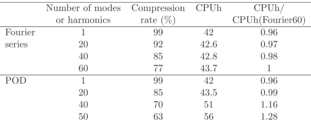
4.2.8 Computational cost . . . 70
4.3 3D URANS simulation of a compressor stage . . . 71
4.3.1 Numerical setup . . . 71 4.3.2 Operating line . . . 72 4.3.3 Flow field . . . 73 4.3.4 Time-averaged values . . . 73 4.3.5 Instantaneous values . . . 75 4.3.6 Computational cost . . . 76
5 URANS simulations at off-design conditions 79 5.1 Use of several blade passages . . . 80
5.1.1 Numerical setup . . . 80
5.1.2 Operating lines . . . 80
5.1.3 Time dependent quantities . . . 80
CONTENTS v
5.1.5 Conclusion . . . 82
5.2 3D simulation of the CME2 stage . . . 82
5.2.1 Numerical setup . . . 82
5.2.2 Mass flow rate . . . 84
5.2.3 Flow field . . . 85
5.2.4 Time-averaged values . . . 88
5.3 Conclusion . . . 89
6 Large-eddy simulation of the flow around a cylinder row 91 6.1 Test case description and numerical setup . . . 91
6.2 Post-processing . . . 92
6.3 Massflow rate . . . 93
6.4 Flow field . . . 93
6.5 Mean flow . . . 93
6.6 Spectrum and vortex shedding . . . 95
6.7 Correlations . . . 98
6.8 Turbulent kinetic energy and Reynolds tensor . . . 99
6.9 Computational cost . . . 99
6.10 Conclusions . . . 105
7 Large-eddy simulation of a compressor stage 107 7.1 Numerical setup . . . 107
7.1.1 Mesh . . . 107
7.1.2 Time and space discretization . . . 108
7.1.3 Boundary conditions . . . 108
7.1.4 Initial conditions . . . 108
7.2 Operating point . . . 108
7.2.1 Massflow rate . . . 108
7.2.2 Performances . . . 108
7.3 Post-processing of the phase-lagged computations . . . 109
7.4 Flow field . . . 110 7.5 Time-averaged values . . . 110 7.6 Computational cost . . . 117 7.7 Conclusion . . . 118 Conclusion 119 Appendix 122 A Treatment of pitch and stage interfaces in elsA 125 A.1 No-match configuration . . . 125
A.2 Stage interfaces . . . 126
A.2.1 Sliding mesh conditions . . . 126
A.2.2 Phase-lagged conditions . . . 126
A.2.3 Profile transformation conditions . . . 126
A.3 Azimuthal interfaces . . . 126
C 1.5 stage simulations 131
C.1 Convection of a hot point . . . 131
C.2 Numerical setup . . . 131
C.2.1 Mesh . . . 131
C.2.2 Time and space discretization . . . 131
C.2.3 Boundary conditions . . . 132 C.3 Single-stage . . . 132 C.4 Multi-stage . . . 132 C.5 Conclusion . . . 134 135 D Article Bibliography 147 156 Résumé Introduction 159
Chapitre 1 : Phénomènes instationnaires et pertes en turbomachine 161 Chapitre 2 : Simulation numérique des écoulements turbulents en turbomachine 163 Chapitre 3 : Choix d’une méthode de compression de donnée pour les signaux
turbulents 167
Chapitre 4 : Validation des conditions aux limites chorochroniques POD pour des 171 simulations URANS d’étages de turbomachines
Chapitre 5 : Simulation URANS d’un étage de turbomachine hors design 177 Chapitre 6 : Simulation aux grandes échelles de l’écoulement autour d’un cylindre179 183 Chapitre 7 : Simulation aux grandes échelles d’un étage de turbomachine
List of Figures
1 Cutaway view of a CFM - LEAP engine. . . 1
1.1 Example of compressor and turbine maps . . . 4
1.2 Absolute and relative velocities across a compressor stage . . . 5
1.3 Losses in a turbomachinery stage . . . 5
1.4 Illustration of natural and bypass transition . . . 6
1.5 Wake in a compressor stage . . . 7
1.6 Illustration of the creation of the tip vortex . . . 9
1.7 Illustration of shock - boundary layer interaction with transition . . . 10
2.1 Simulated and modeled part of the Kolmogorov spectrum for RANS, LES and DNS methods . . . 13
2.2 Illustration of the eddies separation by the mesh grid in large-eddy simulations . . . 15
2.3 Grid requirement for wall-resolved LES in the inner and outer boundary layer . . . . 18
2.4 Illustration of the need of wall modeling when coarse cells are used at wall . . . 19
2.5 Ratio between the number of grid points needed for resolved LES and for wall-modeled LES. . . 20
2.6 Illustration of geometry change method . . . 21
2.7 Illustration of the use of profile transformation . . . 21
2.8 Ratio between the grid requirement for a full annulus simulation and a phase-lagged simulation . . . 22
2.9 Illustration of the consequences of using one blade passage per row . . . 22
2.10 Illustration of spatial and temporal lag in a turbomachinery stage . . . 23
2.11 Relative position of rows A and B at time t = 0 . . . 23
2.12 Memory cost for direct storage . . . 25
2.13 Illustration of the time inclined method . . . 26
3.1 Caption of the flow around a cylinder at different Reynolds number . . . 31
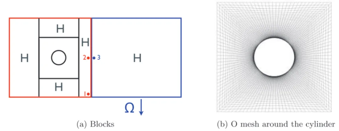
3.2 Illustration of the cylinder row. . . 32
3.3 Mesh configuration of the cylinder case . . . 33
3.4 Entropy field and Fast Fourier Transform of vy in the wake on the stator . . . 34
3.5 Spanwise correlation of vx downstream the cylinder. . . 35
3.6 Three examples of signals extracted from the LES of the flow around a cylinder and their PSD. . . 35
3.7 Relative error on the mean and on the standard deviation obtained with the Fourier series decomposition. . . 38
3.8 Relative error on the mean and on the standard deviation obtained with the discrete Fourier transform. . . 39
3.9 Coefficients and relative error on the mean and on the standard deviation obtained
with the discrete cosine transform. . . 39
3.10 Illustration of the wavelet decomposition process. . . 40
3.11 Relative error on the standard deviation of the signal with discrete wavelet decom-position. . . 40
3.12 Illustration of the creation of the matrix that will be compressed with POD . . . 41
3.13 Compression with Proper Orthogonal Decomposition of a square wave. . . 43
3.14 Error on the standard deviation of the signal with proper orthogonal decomposition. 44 3.15 Influence of the compression algorithms on an axial momentum signal . . . 45
4.1 3D view of the CME2 compressor . . . 48
4.2 Meridional view of the CME2 compressor . . . 49
4.3 Illustration of the throttle law . . . 50
4.4 Illustration of the recomposition of a 2π10 sector after a phase-lagged computation . . 51
4.5 Iso-rotation speed line of the CME2 2.5D test case . . . 51
4.6 Mass flow rate in the CME2 2.5D test case at nominal operating conditions . . . 52
4.7 Normalized entropy and static pressure flow fields at nominal operating conditions . 53 4.8 Position of the interfaces, sections and probes . . . 54
4.9 Instantaneous normalized axial velocity at S1 and S2 . . . 54
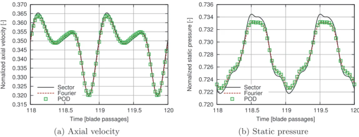
4.10 Time evolution of the axial velocity and the static pressure in the stator passage . . 55
4.11 Fourier transform of the axial velocity and static pressure in the stator passage . . . 55
4.12 Evolution of the pressure ratio and the efficiency with the compression rate . . . 56
4.13 Entropy flow field for different numbers of modes . . . 56
4.14 Normalized axial velocity at S2 with different numbers of modes . . . 57
4.15 Axial velocity and static pressure in the stator passage with different numbers of modes. . . 57
4.16 Ratio σmax σmin between the maximum and the minimum singular values contained in the POD at each phase-lagged interface . . . 58
4.17 Relative error % on ρvx with 2 and 5 modes . . . 59
4.18 Percentage of cells under 1% and 5% of relative error for ρ in the stator . . . 60
4.19 Mass flow rates for the TATEF configuration . . . 63
4.20 Fields of entropy and grad(ρ)ρ . . . 64
4.21 Isentropic Mach for the phase-lagged computations of a transonic turbine stage . . . 64
4.22 Heat fluxes at stator and rotor blade wall . . . 65
4.23 Position of the interfaces, the sections and the probes . . . 66
4.24 Axial velocity over a 3 ×2π64 reconstructed sector . . . 66
4.25 Axial velocity at the probe locations . . . 67
4.26 Fast Fourier transform of the axial velocity at the probe locations . . . 68
4.27 Ratio σmax σmin between the maximum and the minimum singular values contained in the POD . . . 69
4.28 Relative error on ρvx with 2 and 5 modes . . . 70
4.29 Total pressure ratio and efficiency iso-rotation speed line . . . 72
4.30 Mass flow rate at nominal operating point . . . 73
4.31 Reconstructed 2π10 sector shaded with entropy at different blade span . . . 74
4.32 Axial momentum at section S1 and entropy at section S2 . . . 75
4.33 Isentropic Mach number at the stator blade at different blade span . . . 75
LIST OF FIGURES ix
4.35 Position of the probes. . . 76
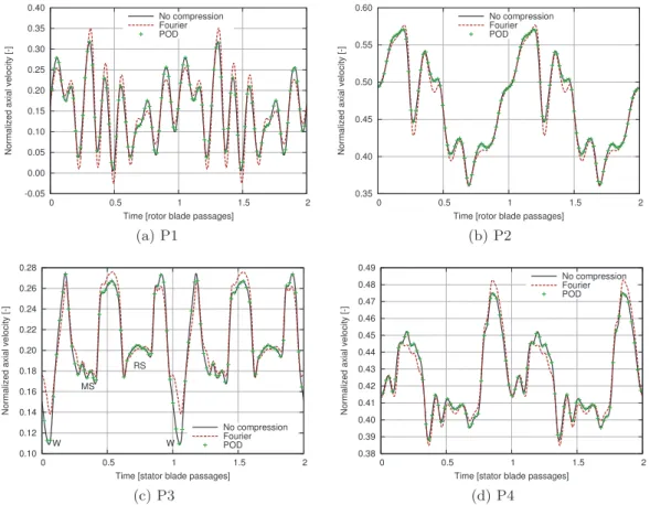
4.36 Axial velocity, static pressure and its spectrum . . . 77
5.1 Total pressure ratio and efficiency obtained with the different configurations at off-design condition. . . 81
5.2 Normalized axial velocity and normalized static pressure in the stator passage at off-design conditions . . . 81
5.3 Normalized entropy and static pressure flow fields . . . 83
5.4 Inlet and outlet mass flow rates . . . 84
5.5 Fast Fourier transform of the inlet and the outlet mass flow rate for the three com-putations . . . 85
5.6 Normalized entropy field over one blade passage obtained with the three computa-tions over 8 stator passages. . . 86
5.7 Normalized entropy extracted at the stator suction side over 8 stator passages. . . . 86
5.8 Normalized entropy flow field obtained at mid-span . . . 87
5.9 Normalized entropy flow field obtained at end-walls . . . 87
5.10 Normalized axial momentum at rotor-stator interface and normalized entropy at stator exit . . . 88
5.11 Isentropic Mach number at stator blade wall at different blade span for the three computations. . . 88
5.12 Absolute flow angle at the rotor-stator interface and downstream the stator blade . . 89
6.1 Position of the rotor probes used for the reconstruction of the signal in the stator frame. . . 92
6.2 Illustration of the reconstruction of a probe in the stator frame. . . 93
6.3 Outlet massflow rates and their average . . . 94
6.4 Normalized entropy flow field . . . 94
6.5 Evolution of the time-averaged normalized axial velocity across a 2π10 sector at the stage interface. . . 95
6.6 Mean value of normalized velocity fluctuations across a 2π30 sector upstream and downstream the stage interface . . . 96
6.7 Power spectral density of tangential velocity fluctuations in the absolute frame of reference out of and into the wake . . . 97
6.8 Power spectral density of the normalized tangential velocity fluctuations into the wake in the stator frame upstream and downstream the stage interface for phase-lagged computations at a rotation speed of Ω 2 . . . 98
6.9 Correlations of the velocity fluctuations out of and into the wake . . . 100
6.10 Turbulent kinetic energy upstream and downstream the stage interface for various configurations . . . 101
6.11 Axial velocity component of the Reynolds tensor upstream and downstream the stage interface for various configurations . . . 102
6.12 Tangential velocity component of the Reynolds tensor upstream and downstream the stage interface for various configurations . . . 103
6.13 Radial velocity component of the Reynolds tensor upstream and downstream the stage interface for various configurations . . . 104
7.1 Inlet and outlet massflow rates and moving average . . . 109
7.2 Computed operating points . . . 109
7.3 Normalized entropy at 50% of blade span . . . 111
7.4 Normalized axial momentum at the rotor-stator interface . . . 112
7.6 Time-averaged absolute flow angle at rotor-stator interface . . . 113
7.7 Turbulent kinetic energy at mid-span upstream and downstream the stage interface . 113 7.8 Reynolds tensor component upstream and downstream the stage interface . . . 114
7.9 Correlation of normalized velocity fluctuations at mid-span across a 2π10 sector . . . . 115
7.10 PSD of vθ at the rotor-stator interface in the rotor and the stator reference frame . . 115
7.11 Power spectral density of tangential velocity fluctuations at different positions in the rotor reference frame upstream and downstream the interface . . . 116
7.12 Power spectral density of tangential velocity fluctuations at different positions for an interpolation with cubic splines or 80th order Legendre polynomial . . . 117
A.1 Illustration of a no-match configuration . . . 125
A.2 Illustration of characteristics relationship. . . 126
C.1 Normalized total temperature profile at the inlet boundary. . . 132
C.2 Inlet and outlet massflow rate and density flow field for the SR configuration . . . . 133
C.3 Inlet and outlet massflow rate for the SRS and RSR configurations . . . 133
C.4 Normalized density flow field for the SRS and the RSR configuration . . . 134
8 Normalized entropy at 50% of blade span . . . 184
Nomenclature
Abbreviation
BPF Blade passing frequency
CME2 Single-stage compressor 2 (compresseur mono-´etage 2) DCT Discrete cosine transform
DFT Discrete Fourier transform DWT Discrete wavelet transform
FSD Fourier series decomposition LES Large eddy simulation
POD Proper orthogonal decomposition
URANS Unsteady Reynolds-averaged Navier–Stokes Dimensionless numbers
Re Reynolds number [−] St Strouhal number [−] Greek Symbols
α Absolute flow angle [rad] β Relative flow angle [rad] ǫ Error [−]
η Efficiency [−]
γ Heat capacity ratio [−] κ Wave number [rad.m−1]
λ Throttle parameter [−] ν Viscosity [m2.s−1] Ω Rotation speed [rpm]
π Total to total pressure ratio [−] ρ Density [kg.m−3]
σ Standard deviation [−] τ Data compression rate [−]
θi Azimuthal position of point i [rad]
θP Blade passage pitch [rad]
Latin letters T Temperature [K] a0,an,bn Fourier coefficients [−] C Correlation [−] c Chord [m] D Diameter [m] E Total energy [J.kg−1]
ft Vortex shedding frequency [Hz]
H Blade height [m] M Mach number [−]
m Mean
Nc Number of cells at the interface [−]
Nh Number of harmonics stored [−]
Nm Number of singular values stored [−]
Ns Number of samples stored [−]
Nper Number of time-steps in one passage period [−]
r Radius [m]
s+, n+, r+ Streamwise, normal and radial wall distances [−] T Blade passage period [s]
t Time [s] U0 Upstream velocity [m.s−1] vi Velocity component [m.s−1] P Pressure [P a] Subscripts θ Tangential quantity
NOMENCLATURE xiii c Compressed data o Original data R Rotor quantity r Radial quantity S Stator quantity s Static quantities t Total quantity x Axial quantity
Abstract
The more and more restrictive standards in terms of fuel consumption and pollution for aircraft engines lead to a constant improvement of their design. Numerical simulations appear as an inter-esting tool for a better understanding and modeling of the turbulent phenomena which occur in turbomachinery. The large-eddy simulation (LES) of a turbomachinery stage at realistic conditions (Mach number, Reynolds number...) remains out of reach for industrial congurations. The phase-lagged method, widely used for unsteady Reynolds-averaged Navier–Stokes (URANS) calculations, is a good candidate to reduce the computational cost. However, it needs to store the signal at all the boundaries over a full passage of the opposite blade. A direct storage of the information being excluded given the size of the mesh grid and timesteps involved, the most used solution currently is to decompose the signal into Fourier series. This solution retains the fundamental frequency of the signal (the opposite blade passage frequency) and a limited number of harmonics. In the frame of a LES, as the spectra are broadband, it implies a loss of energy. Replacing the Fourier series decomposition by a proper orthogonal decomposition (POD) allows the storage of the signal at the interfaces without making any assumptions on the frequency content of the signal, and helps to reduce the loss of energy caused by the phase lagged method. The compression is done by removing the smallest singular values and the associated vectors. This new method is first validated on the URANS simulations of turbomachinery stages and compared with Fourier series-based conditions and references calculations with multiple blades per row. It is then applied to the large eddy simulation of the flow around a cylinder. The error caused by the phase-lagged assumption and compression are separated and it is showed that the use of the POD allows to halve the filtering of the velocity fluctuations with respect to the Fourier series, for a given compression rate. Finally, the large eddy simulation of a compressor stage with POD phase-lagged conditions is carried out to validate the method for realistic turbomachinery configurations.
R´esum´e
Dans un contexte d’am´elioration des moteurs a´eronautiques en termes de consommation et de pol-lution, les simulations num´eriques apparaissent comme un outil int´eressant pour mieux comprendre et mod´eliser les ph´enom`enes turbulents qui se produisent dans les turbomachines. La simulation aux grandes ´echelles (SGE) d’un ´etage de turbomachine `a des conditions r´ealistes (nombre de Mach, nombre de Reynolds. . . ) reste toutefois hors de port´ee dans le cadre industriel. La m´ethode chorochronique, aujourd’hui largement utilis´ee pour les calculs URANS, permet de r´eduire le coˆut des simulations num´eriques, mais elle implique de stocker le signal aux fronti`eres du domaine pen-dant une p´eriode compl`ete de l’´ecoulement. Le stockage direct de l’information ´etant exclu ´etant donn´e la taille des maillages et les pas de temps mis en jeu, la solution la plus courante actuelle-ment est de d´ecomposer le signal sous la forme de s´eries de Fourier. Cette solution ne retient du signal qu’une fr´equence fondamentale (la fr´equence de passage de la roue oppos´ee) et un nombre limit´e d’harmoniques. Dans le cadre d’une SGE, elle implique donc une grande perte d’´energie, et le filtrage des ph´enom`enes d´ecorr´el´es de la vitesse de rotation comme par exemple un lˆacher tourbillonnaire. Le remplacement de la d´ecomposition en s´eries de Fourier par une d´ecomposition aux valeurs propres (POD pour Proper Orthogonal Decomposition) permet de stocker le signal aux interfaces sans faire d’hypoth`ese sur les fr´equences contenues dans le signal et donc de r´eduire la perte d’´energie li´ee `a l’utilisation d’un mod`ele r´eduit. La compression s’effectue en supprimant les plus petites valeurs singuli`eres et les vecteurs associ´es. Cette nouvelle m´ethode est valid´ee sur la simulation URANS d’´etages de turbomachines et compar´ee aux conditions classiques utilisant les s´eries de Fourier et `a des calculs de r´ef´erences contenant plusieurs aubes par roue. Elle est ensuite appliqu´ee `a la simulation aux grandes ´echelles de l’´ecoulement d’un cylindre. Les erreurs caus´ees par l’hypoth`ese chorochronique et par la compression sont s´epar´ees et on montre que l’utilisation de la POD permet de r´eduire de moiti´e le filtrage des fluctuations de vitesses par rapport aux s´eries de Fourier pour un mˆeme taux de compression. Enfin, la simulation aux grandes ´echelles d’un ´etage de turbomachine avec des conditions chorochroniques POD est r´ealis´ee afin de valider la m´ethode dans le cadre d’une configuration industrielle.
Introduction
Context and motivation of the study
In the last decades, air transportation has known an important development. This growth still continues in the XXIth century: the number of people transported has increased by 60% since 2003
and may double in the next 20 years. Meanwhile, pollution, noise, cost and safety issues are becom-ing increasbecom-ingly critical, with ever more restrictive standards. To reach some of these standards, the efficiency of the engine (i.e. its fuel consumption) has to be improved. Indeed, for an A320 airplane, a reduction by 15% of the fuel consumption would represent a saving of 1.4 millions liters of fuel (∼ 1000 cars emissions) and of 3600 tons of CO2 (∼ 240,000 trees absorption) by plane and by year [1]. With almost 20,000 existing airplanes in the world, it thus represents an important economic and environmental issue. After many years of optimization, engine designers need to improve their knowledge of the turbulent flow that sets up in the machine to take the next step.
Figure 1: Cutaway view of a CFM - LEAP engine.
Among the component of a gas turbine, this study focuses on turbines and compressors, which are mobile devices transferring energy between the rotating shaft and the fluid. With the increase of the computational power, computational fluid dynamics (CFD) has appeared to be an interesting way to study flows that can be hard to access with experimental means. Although turbomachinery flows are unsteady and turbulent, steady Reynolds averaged Navier–Stokes (RANS) computations are mainly used in the industry. A first step has been done towards unsteady computations with unsteady-RANS (URANS) simulations. These simulations account for periodic unsteadiness aris-ing, for instance, from the relative motion of the blades and for low frequency instabilities but they still entirely model the turbulence. To overcome this limitation, a solution is the use of large-eddy
simulations (LES), which solves the large eddies of turbulence and models only the smallest ones. However, the LES of a full stage of turbomachinery is about 100 to 10000 times more expensive than a URANS simulation depending on the Reynolds number (Re1.8 [2]) which ranges between
105 and 107 in turbomachinery for aeronautical applications. Such simulations are therefore out of reach in an industrial framework and should not be available before 20 years at current computer power increase rate.
Objectives
The purpose of this work is to explore a way to reduce the cost of large-eddy simulations of turbo-machinery stages by modeling only one blade passage per row. Specific boundary conditions, called the phase-lagged boundary conditions, are applied. These conditions are today widely employed in the industry to achieve URANS simulations. However, they need the use of a data compression method, usually based on the Fourier series decomposition, which only retains a specific frequency and its multiples in the signal. They therefore do not seem adapted for large-eddy simulations where the spectra of the signals are broadband and not composed of discrete frequencies. The objectives of this study are thus:
- to set up phase-lagged boundary conditions using a compression method more adapted to the compression of turbulent signals,
- to study the behavior of phase-lagged boundary conditions with a large-eddy simulations and their advantages and drawbacks,
- to achieve the phase-lagged large-eddy simulation of a compressor stage at nominal operating conditions.
Outline
This thesis is organized in four parts. In a first one, the context of the study is exposed. Some of the flow phenomena that set up in a turbomachinery stage are presented with a particular interest for turbulence. The theoretical background considered to simulate turbulent flows in turbomachinery is then presented, with emphasize on the methods that can be used to reduce the computational cost (like phase lagged approach).
In a second part, several compression methods are evaluated on their ability to preserve the mean, the standard deviation and the spectrum of turbulent signals. Their advantages and draw-backs are compared.
In a third part, the new compression method is verified and validated with 2.5D and 3D URANS computations of a compressor stage and of a transonic turbine stage. The behavior of phase-lagged conditions at off-design conditions is briefly investigated.
Finally, in a fourth part, phase-lagged large-eddy simulations of the flow around a cylinder and of a compressor stage are carried out. The improvement brought by the use of the POD on the filtering of the velocity fluctuations is quantified, different sources of error are identified in such simulations and their limitations are underlined.
Chapter
1
Unsteady phenomena and losses in
turbomachinery
Contents
1.1 Transition . . . 5
1.2 Blade-row interactions . . . 6
1.2.1 Wake interaction . . . 6
1.2.2 Wake-boundary layer interaction . . . 7
1.2.3 Potential effects . . . 7
1.2.4 Clocking . . . 8
1.3 Secondary flows . . . 8
1.3.1 Corner vortex . . . 8
1.3.2 Passage vortex . . . 8
1.3.3 Tip leakage flow . . . 8
1.4 Shock . . . 9
1.4.1 Shock-waves interaction . . . 9
1.4.2 Shock-boundary layer interaction . . . 9
1.5 Off-design operating conditions . . . 10
1.6 Conclusion . . . 10
A turbomachinery is a device where mechanical energy, in the form of shaft work, is transferred either to or from a continuously flowing fluid by the dynamic action of rotating blade rows. A tur-bomachinery stage is composed of a stationary blade row (stator) and a rotating blade row (rotor) in which the transfer is achieved. Work-absorbing turbomachines, where the energy is transferred from the shaft to the fluid, are called compressors (or fans). Work-producing ones are called tur-bines.
A turbomachinery is designed to operate at a nominal operating point which is defined by a rotation speed and a mass flow rate. In these conditions, the performances of the machine are defined by its pressure ratio (compression or dilatation rate):
π= Ptout
Ptin
for compressors and π = Ptin
Ptout
for turbines (1.1)
and its isentropic efficiency:
η= Isentropic compressor work Actual compressor work =
!P tout Ptin "γ−1 γ − 1 !T tout Ttin " − 1
for compressors and (1.2)
η= Actual turbine work Isentropic turbine work =
1 −!Ttout Ttin " 1 −!Ptout Ptin "γ−1γ for turbines. (1.3) However, turbomachines can operate over a range of rotations speed and mass flow rate. The set of all the operating points of a machine define a map. In the compressor case, as illustrated in Fig. 1.1(a), the operating range is limited for a fixed rotation speed (Nn):
- by a maximal mass flow rate, called the chocked mass flow rate. When the flow reaches a certain velocity, a sonic line occurs at the throat of one row (transonic case) or in the inter-blade passage (supersonic case). Then, the maximum mass flow rate that can pass through the machine is reached: it corresponds to the vertical part of the line.
- by a minimal mass flow rate, below which the flow in the machine becomes unstable and phenomena such as rotating stall and surge appear. The line defined by the minimal mass flow rate at each rotation speed is called the surge line.
The turbine map is presented in Fig. 1.1(b). In this case, the operating range is only limited by a chocked mass flow rate.
Operating line Nn Surge line Pressure ratio Massflow (a) Compressor Mass flow Expansion ratio (b) Turbine
Figure 1.1: Example of (a) a compressor map and (b) a turbine map, respectively from Carbon-neau [3] and Ottavy [4]
The flow field in a turbomachinery can be expressed either in a frame linked to the row (relative frame) or to a fixed observer (absolute frame). In the stator case, these two frames are identical. The relative speed W , the absolute speed V and the drive speed U , presented in Fig. 1.2 are linked by:
V = W + U. (1.4)
Absolute and relative angles of the flow are also defined: α = arctan!Vθ VX " β = arctan!Wθ VX " (1.5)
1.1. TRANSITION 5
Mobile row Static row
W V U 2 2 2 2 α β U W1 V 1 α1 β1 3 α Θ X
Figure 1.2: Velocities across a compressor stage, from Ottavy [3]
The operating point of a turbomachinery is characterized by its mass flow rate and its pressure ratio at a given rotation speed. Both are determined by the designer to fit with the whole engine and are constrained by its thermal cycle. To reduce the fuel consumption of the engine, the efficiency has to be improved. For this end, the phenomena responsible for losses in turbomachinery have to be identified and eventually controlled. The purpose of this chapter is to present these phenomena. They are grouped here into four categories: wall effect (laminar-to-turbulent transition), blade row interactions, secondary flows and shocks. The locations of some of these phenomena are presented in Fig. 1.3. In a last section, the reasons why turbomachinery cannot always be operated at their nominal conditions are discussed.
Tip leakage flow Turbulent boundary layer Wake Corner vortex Endwall boundary layer
Figure 1.3: Losses in a turbomachinery stage
1.1
Transition
Laminar-to-turbulent transition is the change of the boundary layer from a laminar state to a turbulent one. It changes the properties of the flow: when the boundary layer is turbulent, the wall friction and the heat transfer are higher and the stall is delayed. Several mechanisms can cause the transition, depending on the Reynolds number, the Mach number, the turbulence rate of the main flow Tu, the pressure gradient, and the roughness and the curvature of the blade:
- natural transition occurs when Tu <1%. Roughness, acoustic waves or the turbulence of the
a critical Reynolds number, these waves are amplified and lead to the formation of turbulent spots and of the turbulent boundary layer. This mechanism is illustrated on Fig. 1.4. - by-pass transition occurs for Tu >1%. In this case the turbulent spots are directly formed
without the apparition of Tollmien-Schlichting waves.
- cross flow transition is caused by transverse instabilities in three dimensional flows.
- in the bubble transition the laminar boundary layer is stalled. Instabilities appear that lead to its transition and its re-attachment. The length of the bubble depends on the Reynolds number.
Laminar Transition Turbulent U Stable laminar flow Not in bypass transition Turbulent spots Fully turbulent flow TS waves Spanwise vorticity 3D breakdown
Figure 1.4: Illustration of natural and bypass transition, from White [5]
The prediction of transition is thus important for the estimation of the losses and is strongly linked to the prediction of the turbulence in the main flow and in the boundary layer.
1.2
Blade-row interactions
Blade-row interactions are unsteady phenomena caused by the relative motion of the rows. The part of each phenomenon in the total amount of loss in a turbomachinery depends on the configuration, however, Yoon et al. [6] estimate that blade-row interactions are responsible for 10% of the loss in a turbine stage.
1.2.1 Wake interaction
A wake is a viscous effect caused by the merging of the boundary layer of pressure and suction sides. It propagates downstream with the flow velocity and is characterized by a velocity deficit area as illustrated of Fig. 1.5.
The experimental work by Soranna et al. [7] showed that the wake modifies the velocity field around the downstream blade even if it does not impinge it. When it reaches the leading edge of the downstream blade, the wake is chopped and convected in the inter-blade channel. This slicing and its consequences on the aerodynamic quantities of the flow have been studied by Mailach et al [8, 9]. Three effects determine the structure of the wake:
- the viscous mixing with the main flow, that tends to widen the wake and to reduce the velocity deficit,
1.2. BLADE-ROW INTERACTIONS 7
- a stretching caused by the enlargement of the inter-blade passage (in a compressor), or a reducing if the section decreases,
- and a mass transport in the blade-to-blade plan, from the pressure side of a blade to the suction side of the adjacent blade. This phenomena, caused by the slip velocity between the main flow and the wake, is called negative jet.
A wake can be defined by its velocity deficit, expressed in % of the free-stream velocity, and its width, measured at mid-deficit. Vortex shedding also appears at the trailing edge of the blade. This phenomena is more described in chapter 3 (in the case of a cylinder). Its frequency depends on the diameter of the trailing edge, the viscosity and the velocity of the flow. It is thus not correlated from the blade passing frequency.
stator
rotor
SS PS
flow
Figure 1.5: Wake in a compressor stage, from Mailach et al. [8]
Turbulence affects the interaction of the wake with the main flow. Indeed, the turbulence rate influences the mixing of the wake and the main flow and thus the creation of loss. The wake itself is turbulent and its state depends on the transition of the boundary layer at the blade wall. In addition, the shear stress between the wake and the main flow create turbulence.
1.2.2 Wake-boundary layer interaction
The passing wakes coming from the upstream blade can interact with the boundary layer on the downstream blade and trigger the laminar-to-turbulent transition. As this phenomenon is periodic, the boundary layer is composed of a turbulent area, followed by a medium zone called ‘calmed’ before turning back to a laminar state. If the wakes are passing quickly enough, the boundary layer never gets the time to become laminar again and it stays turbulent. This delays its separation and has a stabilizing effect for the machine [10]. Ottavy et al. [11] and Wheeler et al. [12] studied this phenomena in axial compressor and showed that it can be beneficial in terms of performances but it is highly sensitive to the incoming flow and to the shape of the leading edge.
1.2.3 Potential effects
The potential effects are created by the presence of an obstacle in the flow (here, the blades), and they are assimilated to pressure forces. They propagate upstream and downstream at the speed of sound. The rotor-stator interaction therefore reorganizes quasi-instantaneously the pressure field. It is difficult to separate a priori the potential effect coming from the upstream and downstream rows, but Mailach et al. [13] showed that the one coming from the downstream row is dominating.
The intensity of the potential effect decays with the distance and Leboeuf [14] proposed the following expression: ∂P ρU2 # # # # max = $ 1 − M2 1 − M2x exp % −2π $ 1 − M2 1 − M2x x θP & . (1.6)
Where M is the Mach number, p the pressure, U the velocity magnitude and θP the blade passage
pitch. When the distance from the blade θx
P is important, it is strongly attenuated. In current
turbomachinery, the trend is to decrease the distance between the rows to address size constraints and to increase the blade loading. This leads to an increase of the potential effects. However, they remain one order of magnitude lower than the wake interaction effects [15].
1.2.4 Clocking
Clocking is the interaction between rows rotating at the same rotation speed and their consequences on the performances of multi-stages configurations. For a 1.5 stage turbine where the two stator rows have the same number of blades, the efficiency is maximum when the wake of stator 1 impinges stator 2 at its leading edge because it decreases the velocity around the blade [16]. Conversely, the efficiency is minimized when the wake impinges the blades in the inter-blades passage.
1.3
Secondary flows
In secondary flows, the flow field is different in speed and direction from the majority of the domain and to what is predicted for an inviscid fluid. These phenomena are responsible for one third of the total losses [17].
1.3.1 Corner vortex
The strong adverse pressure gradients at the foot of the blade caused by the interaction of the boundary layers of the hub and of the suction side of the blade can cause a stall and create a vortex. This vortex creates a flow opposed to the main flow of the stage and is responsible for aerodynamic losses and a deviation of the flow [18][19].
1.3.2 Passage vortex
The passage vortex is caused by the flow deviation induced by the blades. In the boundary layers at the hub and at the casing, the velocity is less important. These areas are therefore more sensitive to the pressure gradient between the pressure and the suction sides of the blade. A radial flow is induced toward the endwalls at the pressure side and from the endwalls at the suction side and thus a recirculation from the suction side toward the pressure side at mid-span. This leads to the creation of the passage vortex.
1.3.3 Tip leakage flow
Between the tip of a mobile blade and the casing, there exist a tiny space called the tip gap. Flow is therefore moving in this gap from the pressure side towards the suction side as illustrated on Fig. 1.6. The tip leakage flow is normal to the main-flow direction and their mixing results in the creation of entropy and losses. A vortex sheet is also created in the upstream part of the blade and convected, resulting in the creation of tip vortices. The turbulent mixing of the tip leakage flow with the main flow is responsible for losses and has an important impact on the machine stability [20, 21, 22]. In addition, in this area the turbulence is not isotropic.
1.4. SHOCK 9
Main flow Tip vortex
Vortices sheet
Tip leakage flow
Tip vortex path
Figure 1.6: Illustration of the creation of the tip vortex, from Leboeuf [14]
1.4
Shock
A shock is a discontinuity that appears in transonic or supersonic flows and its thickness is of the order of size of the mean free path of molecules. Across a shock, the Mach number and the total pressure decrease, while the static pressure and the static temperature increase. For example, assuming a normal shock in a flow at M=1.4, which is representative of turbomachinery conditions, the loss of total pressure is of 4%.
1.4.1 Shock-waves interaction
In a transonic turbomachinery, shock waves appear. They can reflect on upstream and downstream rows and can interfere with the other unsteadiness caused by the rotor-stator interactions. Ottavy et al. [23] studied the impact of a shock wave on the wake of the inlet guide vane. Before the shock passage, the velocity deficit and the flow deviation are increased. The reversed phenomenon happens after the passage of the shock. Gorell et al. [24][25] showed that in a similar configuration, the shock at the leading edge of the rotor is chopped by the upstream stator row. This causes a pressure wave (normal to the stator blade), which leads to a decrease of the performances. Shock waves can also interact with the wakes of the upstream or the neighbor blades, resulting in their bending and their oscillation [26].
1.4.2 Shock-boundary layer interaction
The shock at the trailing edge of the upstream row impinges the downstream blade and operates a retrograde sweeping. It can cause the development of a separation bubble at the foot of the shock and eventually the transition of the boundary layer for compressor configurations [27, 28], as illustrated on Fig. 1.7. The boundary layer can eventually relaminarizes downstream the shock [29]. When it is already turbulent, the shock-boundary layer interaction can trigger the stall. The behavior of the shock is related to the state of the boundary layer and thus to the good prediction of the laminar-to-turbulent transition.
Sonic line
Main shock
Compression waves
Secondary shock
Laminar b. l.
Laminar separation Transition to turbulence
Figure 1.7: Illustration of shock - boundary layer interaction with transition, from Carbonneau et al. [30].
1.5
Off-design operating conditions
The engine can operate at conditions in which its efficiency is not maximal for several reasons. On the one hand, instabilities appear in compressor at low mass flow rates, which can result in important damages for the machine. Indeed, at low mass-flow rate, the flow angle upstream the blades increases. This causes the boundary layer to become wider and eventually block the flow in the inter-blade passage, creating stalled cell. The flow is deviated toward the adjacent blades, increasing the incidence on the blade located at the pressure side. This neighbor blade is blocked in its turn and thus the stalled cell moves from one blade to another. It rotates at 30 to 80% of the rotating speed. There can be one or several cells in the machine and they can cover all or a part of the blade span. This phenomena is called rotating stall and is acknowledged to be a precursor of surge.
The surge of a compressor is an axial oscillation of the flow at low frequency (1 to 100 Hz) that can lead to the set up of a reverse flow and to a failure of the machine [31, 32]. To prevent the compressor from entering these operating conditions, the designer thus uses a safety margin, called the surge margin.
On the other hand, there are uncertainties in the operating conditions, especially the inlet flow field, which can experience variations or non-homogeneities. It leads to an overestimation of the surge margin and sometimes the maximum efficiency operating point cannot be used.
1.6
Conclusion
Some phenomena responsible for losses in turbomachinery have been presented in this chapter. Many of them involve turbulence, like the mixing of the wakes, wake-boundary layer interaction, shock-boundary layer interaction and tip leakage flows. An accurate prediction of these phenomena will lead to a progress of their knowledge and understanding and thus to a potential improvement of engines efficiency.
Chapter
2
Numerical simulation of the turbulent flow in
turbomachinery
Contents
2.1 Navier–Stokes equations . . . 12
2.2 Numerical simulation of turbulence in turbomachinery . . . 13
2.2.1 Direct numerical simulations . . . 13
2.2.2 (U)RANS simulations . . . 13
2.3 Large-eddy simulations . . . 15
2.3.1 Filtered equations . . . 15
2.3.2 Subgrid scales models . . . 16
2.3.3 Boundary conditions . . . 17
2.3.4 Mesh grid . . . 17
2.4 Methods to mitigate the mesh requirement for LES . . . 18
2.4.1 Wall modeling . . . 19
2.4.2 Reduction of the number of blade passages . . . 19
2.4.3 Phase-lagged boundary conditions . . . 21
2.4.4 Conclusion on the reduction of the mesh size for large eddy simulation . . . 27
Turbomachinery experience unsteady and turbulent flows. The future of aeronautics engines, based on their improvement or a technological breakthrough, requires a better understanding of these structures. In the past decades, with the emergence of supercomputers, numerical simulations have arisen as an interesting solution to study the turbulent phenomena in turbomachinery. The aim of this chapter is thus to present some of the existing methods for the numerical simulation of the turbulent flow in turbomachinery and to look among them for a trade-off between the computational cost and the range of turbulent eddies solved for complex configurations at high Reynolds numbers.
The governing equations for turbulent flows are presented in a first section. Different methods to numerically model them are reviewed in a second one. These methods differ from each other by the range of turbulent eddies they model or resolve. The relative cost of each one is discussed. Then, in a third part, methods that allow the reduction of the mesh size are presented.
2.1
Navier–Stokes equations
The Navier–Stokes equations describes the three-dimensional flow of a non-reactive, single-phase, Newtonian, compressible fluid. These equations result from the mass (Eq. 2.1), momentum (Eq. 2.2) and total energy (Eq. 2.3) conservation. As they are applied here to the airflow in turbomachinery, the volume forces are neglected.
Conservation of mass: ∂ρ ∂t + ∂ ∂xj (ρuj) = 0 (2.1) Conservation of momentums: ∂ρui ∂t + ∂ ∂xj [ρuiuj + pδij − τij] = 0 i = 1,2,3 (2.2)
Conservation of total energy:
∂ρE ∂t +
∂ ∂xj
[ρEuj+ ujp+ qj− uiτij] = 0 (2.3)
Where ρ is the density, ui the components of the velocity and E the total energy. To close these
equations, it is necessary to determine the pressure p, the stress tensor τ , the dynamic viscosity µ and the heat flux q. In this purpose, the following state laws and behavior laws are used.
The ideal gas law connects the thermodynamic properties of the fluid. It expresses p as:
p= ρrT , (2.4)
where T is the temperature and r is the specific gas constant (r = 287.058 J.kg−1.K−1). For a Newtonian fluid, the stress tensor yields:
τij = µ ' ∂ui ∂xj +∂uj ∂xi − 2 3 ∂uk ∂xk δij ( . (2.5)
The Sutherland law gives the viscosity of the fluid:
µ(T ) = µ0' T
T0
(32
T0+ 110.4
T + 110.4, (2.6)
with, for air, µ0 = 1.711 × 10⁻⁵ kg.m.s−1 and T0 = 273.15 K.
At last, the Fourier law gives the heat flux q:
qj = −λ
∂T ∂xj
, (2.7)
with λ the thermal conductivity of the fluid which is given by: P r = µCp
λ = 0.72 for air where Cp
is the heat capacity of the fluid.
These equations have no known analytical solution and are thus discretized to be numerically solved. The discretized equations can then be directly solved or filtered in order to model all or only a part of the turbulence. Different solutions to numerically simulate the turbulent flows in turbomachinery are presented in the next section.
2.2. NUMERICAL SIMULATION OF TURBULENCE IN TURBOMACHINERY 13
2.2
Numerical simulation of turbulence in turbomachinery
Different methods exist to capture the turbulent scales of the flow. Three of them are presented in the next paragraphs. These methods differ from each other by the range of turbulent eddies they model and resolve. They are ranging from total simulation (DNS) to total modeling (RANS). Intermediate solutions exist, such as large-eddy simulations (LES). Figure 2.1 presents these meth-ods.
Figure 2.1: Simulated and modeled part of the Kolmogorov spectrum for RANS, LES and DNS methods. From Gravemeier [33].
2.2.1 Direct numerical simulations
Direct numerical simulation (DNS) solves all the turbulent scales. To achieve this, the size of the mesh cells has to be of the order of the smallest scale of turbulence η. The domain modeled also has to be at least of the size of the largest scale L, which is of the magnitude of the size of the obstacle. It can be shown [34] that Lη ∽Re34 where Re = ρU L
µ is the Reynolds number based on the
size of the largest scales. As the domain is three dimensional, this means that the number of cells needed is of magnitude Re94. Given that the Reynolds numbers existing in industrial compressors
are about 106, simulations of 3D full turbomachinery stages are today unreachable. However, there are some examples in the last years of DNS of single blades operating at low Reynolds Number. For example, Wissink and Rodi [35], Wissink et al. [36] and Wheeler et al. [37] performed DNS at Reynolds number ranging from 72,000 to 570,000. But in all these cases the modeled blade span does not exceed 0.25 chord (0.1 chord for the DNS of Wheeler). There are very few example of DNS of a full stage, like the turbine stage computed by Rai [38] at Re = 100,000. The existing DNS thus concern simplified configurations operating at low Reynolds numbers.
2.2.2 (U)RANS simulations
2.2.2.1 Averaged equations
In Reynolds-averaged Navier–Stokes (RANS) simulations, a Reynolds averaged flow, corresponding to a statistic average of several realization of the flow, is computed. This averaging filters the random fluctuations of the flow and the effects of turbulence are entirely modeled. When the flow is not steady, a phase-average is achieved in order to take into account the unsteadiness linked to
the motion of the blades (URANS approach). These simulations capture the unsteady periodic phenomena that occur in turbomachinery. The assumption of ergodicity is done, which states that a temporal averaging and a statistic averaging are equivalent. For RANS simulations, the averaging is performed over the whole time of the flow. For URANS simulations it is done on a sufficiently short time that the periodic interactions are kept while the turbulent eddies are filtered. The unsteady Reynolds averaged Navier-Stokes (URANS) equations yields:
∂ρ ∂t + ∂ ∂xj (ρuj) = 0 (2.8) ∂ρui ∂t + ∂ ∂xj ) ρuiuj+ pδij− τij+ 2 3µt ∂uj xj − 2µt S * = 0 i = 1,2,3 (2.9) ∂ρE ∂t + ∂ ∂xj ) + ρE+ p,uj − ' τ −2 3µt ∂uj ∂xj + 2µtS ( uj+ q + qt * = 0 (2.10)
where ¯. is the Reynolds averaging operator and ¯S is the mean rate of strain tensor.
2.2.2.2 Closure of the equations
To close these equations, two kinds of possibilities exist. With first order models, that rely on the Boussinesq approximation, an expression is given for µt. It can be done with an algebraic model,
which directly links µt to the mean flow without adding any transport equation. An example of
such model is the Baldwin and Lomax model [39]. Another solution consists in adding one or two equations in the system to transport the turbulent kinetic energy k and eventually an other quantity. This is the case in the Spalart–Almaras model [40] (1 equation), or in the k − ω Wilcox model [41] and the k − l Smith model [42] (2 equations). With second order models, the transport equations for the Reynolds stress tensor are solved. This solution adds 6 equations for the double correlations and a seventh for a length scale, usually the turbulent dissipation rate. The Reynolds Stress Model of Launder et al. [43] is an example of second order model. First order models rely on the assumptions of isotropy and equilibrium of the turbulence, which are not always true in turbomachinery. However, the transport of the 6 double correlations of the Reynolds stress tensor induces an important increase of the computational cost. To reduce this cost and still overcome the isotropy assumption, some models propose an algebraic solution, like the EARSM model by Wallin and Johansson [44]. The solution is sensitive to the choice of the turbulence model [45][46]. Indeed, each model is calibrated to handle a specific kind of flow and can barely be used for another one.
2.2.2.3 Transition modeling
As turbulence is modeled, the transition of the boundary layer cannot be simulated. The user can thus either assume that the flow is fully turbulent (which is usually not true as seen in section 1.1) either use a transition model. Numerous methods have been proposed to set up a transition crite-rion, and many of them have known several improvement through the time. Four kinds of methods can be distinguished. The eN method relies on a criterion of amplification of the perturbations
in the boundary layer which is linked to the turbulence rate by Mack [47]. Local criteria, as the Abu-Ghannam and Shaw [48] criteria and the C1 transverse one, have a lower computational cost because they use only local information but they do not take into account the history of the boundary layer. On the other hand, a non-local criterion as the Arnal–Habiballah–Delcourt one, implies that the topology of the case is known. At last there are models with one or more transport equations like the Menter and Langtry γ − Reθ [49]. They propose a transport equation for the
intermittency criterion γ, which models the progressive transition from laminar to turbulent. The advantage of these models is that they both are local and account for the boundary layer history.
2.3. LARGE-EDDY SIMULATIONS 15
2.2.2.4 Conclusion on URANS simulations
(U)RANS simulations are currently widely used in the industry and have shown satisfactory results. However their main drawback is that they rely on models (turbulence, transitions) that need to be calibrated and that are often designed for a specific kind of flow. The use of direct numerical simulation, which is free of these models, has been found to be highly expensive. A third solution is presented in the next paragraph, which solves a part of the turbulence and thus reduces the weight of the turbulence model.
2.3
Large-eddy simulations
2.3.1 Filtered equations
The large-eddy simulation solves the large, energetic structures of the turbulence and models the small ones. The separation of the eddies is done with a high-pass filter. This filter can be either explicitly expressed or implicitly done by the mesh grid as illustrated in Fig. 2.2. The structures that are larger than a grid cell are solved and the other ones are modeled. If ∆ is the characteristic length of the mesh in the directions (i,j,k) then the cutting wave number of the filter is:
κc = 2π λc = π ∆, (2.11) with ∆ = (∆i∆j∆k) 1 3. (2.12)
Grid
points
Sub-grid structures
Resolved structures
Figure 2.2: Illustration of the eddies separation by the mesh grid in large-eddy simulations. From Raverdy [50]
All the structures with a wave number above κc are modeled. The other ones are solved. This
filter is applied on the instantaneous flow. A quantity f is decomposed into a resolved part ˜f and a modeled part f′:
f = ˜f+ f′. (2.13)
The ˜. operator is mass pondered:
˜ f = ρf
The filtered equations yield: ∂ρ ∂t + ∂ ∂xj (ρ˜uj) = 0 (2.15) ∂ρ˜ui ∂t + ∂ ∂xj [ρ˜uiu˜j+ pδij − τij − tij] = 0 i=1,2,3 (2.16) ∂ρ ˜E ∂t + ∂ ∂xj [ρ ˜Eu˜j+ ˜ujp+ ˜qj+ θj − ˜uiτ˜ij− ˜uitij] = 0 (2.17)
where tij is the subgrid scale (SGS) stress tensor and θj the subgrid scale heat flux. Because of
these two terms, the filtered equations are not closed. Subgrid scale models are used to model the effect of the smallest eddies.
Various parameters, that will influence the quality of a large-eddy simulation, have to be chosen by the user, like the SGS model or the size of cells that will determine the filter. They are presented in the next paragraphs.
2.3.2 Subgrid scales models
When an explicit filtering of the equations is used, there is no need for subgrid scale modeling. For implicit filtering, two approaches exist:
- implicit methods, in which the dissipation linked to the smallest scales of turbulence is done by the numerical schemes,
- explicit methods, in which these terms are modeled. This kind of method is the most widely used.
Among the explicit methods, there are structural models where the subgrid flow is computed and which are not discussed here, and the functional methods. In the last ones the effect of the subgrid is estimated by expressing tij and θj. The most common models introduce a turbulent
viscosity νSGS. tij = ρνSGS ' ∂˜ui ∂xj +∂u˜j ∂xi − 2 3 ∂u˜k ∂xk δij ( (2.18) θj = ρνSGSCp PrSGS ∂ ˜T ∂xj (2.19) 2.3.2.1 Smagorinsky model
The Smagorinsky sub-grid scale model [51] expresses the sub-grid viscosity as:
µSGS = ˜ρ(Cs∆)2|| ˜S|| (2.20)
where Cs is the Smagorinsky constant and
|| ˜S|| =
-2 ˜SijS˜ij. (2.21)
Assuming that the turbulence is homogeneous and isotropic and that there is an equilibrium between the production and the dissipation of turbulence, this constant can be set to Cs = 0.18.
But Fujiwara et al. [52] showed that near the walls, this model is too dissipative and the transition of turbulence is badly predicted. Some authors thus use lower values for the Smagorinsky constant like Leonard et al. [53] (Cs = 0.09) or McMullan and Page [54] (Cs = 0.1). Dynamic versions of
the Smagorinsky model have been proposed, like that of Germano et al. [55] in which the value of the constant is adapted to each point of the grid mesh depending on the flow physics.
2.3. LARGE-EDDY SIMULATIONS 17
2.3.2.2 WALE model
In the WALE model [56], the sub-grid viscosity yields:
µSGS = (Cw∆)2 SijdSijd ( ˜SijS˜ij) 5 2 + (Sd ijSijd) 5 4 (2.22) with Sijd = 1 2(˜g 2 ij− gji2) − 1 3δijg˜kk 2 and g˜2 ij = ∂˜ui ∂xk ∂˜uk ∂xj . (2.23)
The recommended value for the WALE constant Cw is 0.5. This model respects the cubic decrease
of the sub-grid scale viscosity µSGS with the wall distance.
2.3.2.3 Implicit LES
Implicit LES does not use a sub-grid scale model and assumes that the numerical dissipation is sufficient. It is sometimes called numerical LES (NLES) [57]. If the schemes used are dissipative, the use of a SGS model can lead to an overestimation of the dissipation. But if they are not, it can be required for the stability of the code. Eastwood et al. [58] studied the effect of a change of SGS model on the velocity and shear stress in a jet flow. They concluded that if the code used is dissipative, the choice of the SGS model has little importance and that it can be omitted. Indeed, as 90% of the turbulent kinetic energy is resolved, the modeling of the other 10% has a limited influence[59]. This kind of method has been successfully applied to turbomachinery configurations [58][60]. However, these results are highly dependent on the numerical scheme used.
2.3.3 Boundary conditions
Most applications use non-reflective conditions to avoid parasite pressure waves, especially for acoustic applications. In this case, sponge layers are often used at the exit boundary. No-slip and adiabatic conditions are usually used at blade walls for compressor and isothermal wall conditions for turbines when heat transfer is considered. An important point is the choice of the inlet turbulent rate. According to McMullan and Page [54], an accurate description of the transient flow at the inlet boundary is essential for the fidelity of the simulation. Gourdain et al. [61] and Matsuura and Kato [60] studied the influence of the inlet turbulence rate. They both concluded that inlet conditions are of primary importance for the prediction of the boundary layer state, its transition and its separation. These authors proposed several methods for turbulence injection: turbulence recycling [54], synthetic-eddy method [62] or injection of the previous turbulent simulation of an empty box [60]. However, they all require an a priori knowledge of the turbulence characteristics or a previous simulation, while the turbulent state of the inlet flow is usually badly known.
2.3.4 Mesh grid
Geometry definition and mesh refinement are the most important elements of a LES, according to Tucker [63]. Several studies show that LES is much more sensitive to the grid mesh definition than (U)RANS [27][53]. Indeed, an under-resolved LES badly predicts the gradients near walls and, in this case, Eastwood et al. [58] show that it is better to use a hybrid-LES method than pure LES.
Fig. 2.3 is adapted by Tucker et al. [2] from Piomelli and Balaras [64]. It plots the number of boundary layer grid points (N) needed for one blade passage against the Reynolds number based on the chord Rec. The long and short dashed line stand respectively for the number of grid points
needed in the inner boundary layer (y+ <100) and in the outer boundary layer (δ+ > y+ >100,
At Rec ≈ 105 and below, the inner boundary layer mesh requirement is not dominant and the
order of magnitude of grid points needed is given by N = 3000 ×wc × Re0.4c where w is the span and
cis the chord. This concerns low-pressure turbines. Above Rec≈ 5 × 10⁵, the inner boundary layer
requirement is dominant. This is the case for fans and compressors. Then, an order of magnitude of the total points number needed is N = 5 × 10⁻⁴×wc × Re1.8c .
The points plotted in Fig. 2.3 correspond to simulations of other authors gathered by Tucker [2]. It can be seen that most of them are below the requirements. Indeed a fully resolved LES is highly expensive. This is why today most of the applications are not done with a full 3D geometry but with a simplified one. Indeed, the end walls (and thus the tip gap) are usually not modeled and / or only one isolated blade is computed. In addition, the meshes often do not match the recommended criteria for LES, and under-resolved grids are mostly used.
104 105 106 107 108 109 1010 1011 1012 1013 1014 104 105 106 107 108 109 N c/w Re Total y+<100 y+>100
Figure 2.3: Grid requirement for wall-resolved LES in the inner and outer boundary layer depending on the Reynolds number. Adapted by Tucker et al. [2] from Piomelli and Balaras [64]
Conclusion on LES
Large eddy simulation could be a good trade-off to avoid the use of restrictive assumptions on the turbulence and obtain a better description of the physical phenomena occurring in turbomachinery than with URANS simulations. LES has already been successfully applied to a wide range of turbomachinery problems, such as off-design operating conditions [65][54], secondary flows [66], heat transfer [67][61], and aero-acoustics [68]. However, these simulations still remain expensive and large eddy simulations of a full turbomachinery stage are far from being the norm. If low-pressure turbine computations are emerging, simulations of full 3D compressor stages at realistic Reynolds are quite rare. If the Moore law keeps being followed, such simulations could be available by 2035 [69]. However, experience shows that the size of the meshes is not increasing at the same rate as computing power [69]. One way to reduce this waiting time is to try to reduce the size of the mesh grids.
2.4
Methods to mitigate the mesh requirement for LES
The next paragraphs present several existing methods to reduce the size of mesh grids in large-eddy simulations. Two categories are stressed. On the one hand, there are wall-modeling methods which propose to increase the size of the cells near walls. On the other hand, there are methods that propose to reduce the number of blades passages computed.


![Figure 3.1: Caption of the flow around a cylinder at different Reynolds number by Taneda [107].](https://thumb-eu.123doks.com/thumbv2/123doknet/3106632.88159/51.892.131.804.279.447/figure-caption-flow-cylinder-different-reynolds-number-taneda.webp)