https://doi.org/10.5194/essd-11-129-2019 © Author(s) 2019. This work is distributed under the Creative Commons Attribution 4.0 License.
The AlborEX dataset: sampling of sub-mesoscale
features in the Alboran Sea
Charles Troupin1, Ananda Pascual2, Simon Ruiz2, Antonio Olita3, Benjamin Casas2, Félix Margirier4, Pierre-Marie Poulain5, Giulio Notarstefano5, Marc Torner6, Juan Gabriel Fernández6, Miquel Àngel Rújula6, Cristian Muñoz6, Eva Alou6, Inmaculada Ruiz6, Antonio Tovar-Sánchez7, John T. Allen6,
Amala Mahadevan8, and Joaquín Tintoré6,2
1GeoHydrodynamics and Environment Research (GHER), Freshwater and OCeanic science Unit of reSearch (FOCUS), University of Liège, Liège, Belgium
2Instituto Mediterráneo de Estudios Avanzados (IMEDEA, CSIC-UIB), Esporles, Spain
3Institute for Coastal Marine Environment-National Research Council (IAMC-CNR) Oristano, Oristano, Italy 4Sorbonne Universités (UPMC, Univ Paris06)-CNRS-IRD-MNHN, Laboratoire LOCEAN, Paris, France
5Istituto Nazionale di Oceanografia e di Geofisica Sperimentale (OGS), Trieste, Italy 6Balearic Islands Coastal Observing and Forecasting System (SOCIB), Palma de Mallorca, Spain
7Instituto de Ciencias Marinas de Andalucía, (ICMAN – CSIC), Puerto Real, Spain 8Woods Hole Oceanographic Institution, Woods Hole, MA, USA
Correspondence:Charles Troupin ([email protected]) Received: 31 August 2018 – Discussion started: 3 September 2018
Revised: 25 December 2018 – Accepted: 4 January 2019 – Published: 25 January 2019
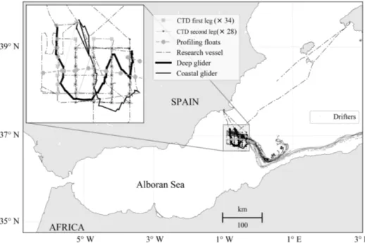
Abstract. The AlborEX (Alboran Sea Experiment) consisted of a multi-platform, multi-disciplinary experiment carried out in the Alboran Sea (western Mediterranean Sea) between 25 and 31 May 2014. The observational component of AlborEx aimed to sample the physical and biogeochemical properties of oceanographic features present along an intense frontal zone, with a particular interest in the vertical motions in its vicinity. To this end, the mission included 1 research vessel (66 profiles), 2 underwater gliders (adding up 552 profiles), 3 profiling floats, and 25 surface drifters.
Near real-time ADCP velocities were collected nightly and during the CTD sections. All of the profiling floats acquired temperature and conductivity profiles, while the Provor-bio float also measured oxygen and chlorophyll a concentrations, coloured dissolved organic matter, backscattering at 700 nm, downwelling irradiance at 380, 410, and 490 nm, as well as photo-synthetically active radiation (PAR).
In the context of mesoscale and sub-mesoscale interactions, the AlborEX dataset constitutes a particularly valuable source of information to infer mechanisms, evaluate vertical transport, and establish relationships be-tween the thermal and haline structures and the biogeochemical variable evolution, in a region characterised by strong horizontal gradients provoked by the confluence of Atlantic and Mediterranean waters, thanks to its multi-platform, multi-disciplinary nature.
The dataset presented in this paper can be used for the validation of high-resolution numerical models or for data assimilation experiment, thanks to the various scales of processes sampled during the cruise. All the data files that make up the dataset are available in the SOCIB data catalog at https://doi.org/10.25704/z5y2-qpye (Pascual et al., 2018). The nutrient concentrations are available at https://repository.socib.es:8643/repository/ entry/show?entryid=07ebf505-bd27-4ae5-aa43-c4d1c85dd500 (last access: 24 December 2018).
1 Introduction
The variety of physical and biological processes occurring in the ocean at different spatial and temporal scales requires a combination of observing and modelling tools in order to properly understand its underlying mechanisms. Hydrody-namical models make it possible to design specific numer-ical experiments or simulate an idealised situation that can reproduce some of these processes and assess the impacts of climate change. Despite the continuous progress made in modelling (spatial resolution, parameterization, atmospheric coupling, etc.), in situ observations remain an essential yet challenging ingredient when addressing the complexity of the ocean.
To properly capture and understand these small-scale fea-tures, one cannot settle for only observations of temperature and salinity profiles acquired at different times and positions, but rather one has to combine the information from diverse sensors and platforms acquiring data at different scales and at the same time, similarly to the approach described in Delaney and Barga (2009). This also follows the recommendation for the Marine Observatory in Crise et al. (2018), especially the co-localisation and synopticity of observations and the multi-platform, adaptive sampling strategy. We will refer to these as multi-platform systems, as opposed to experiments artic-ulated only around the observations made using a research vessel. Further details can be found in Tintoré et al. (2013).
The western Mediterranean Sea is a particularly relevant region for multi-platform experiments, thanks to the wide range of processes taking place, which have been intensively studied since the work of Wüst (1961) on vertical circula-tion: for example, influence on climate (e.g. Giorgi, 2006; Giorgi and Lionello, 2008; Adloff et al., 2015; Guiot and Cramer, 2016; Rahmstorf, 1998) and sea-level change (e.g. Tsimplis and Rixen, 2002; Bonaduce et al., 2016; Wolff et al., 2018), thermohaline circulation (e.g. Bergamasco and Malanotte-Rizzoli, 2010; Millot, 1987, 1991, 1999; Skliris, 2014; Robinson et al., 2001), water mass formation and con-vection process (e.g. MEDOC-Group, 1970; Stommel, 1972; Send et al., 1999; Macias et al., 2018), and mesoscale (e.g. Alvarez et al., 1996; Pinot et al., 1995; Pujol and Larnicol, 2005; Sánchez-Román et al., 2017) and sub-mesoscale pro-cesses (e.g. Bosse et al., 2015; Damien et al., 2017; Mar-girier et al., 2017; Testor and Gascard, 2003; Testor et al., 2018). Other recent instances of multi-platform experiments in the Mediterranean Sea were focused on the Northern Cur-rent (December 2011, Berta et al., 2018), deep convection in the northwestern Mediterranean sea (July 2012–October 2013, Testor et al., 2018), the Balearic Current system (July and November 2007, April and June 2008, Bouffard et al., 2010) and the coastal current off the west of Ibiza (August 2013, Troupin et al., 2015). Similar studies comparing almost synchronous glider and SARAL/AltiKa altimetric data on se-lected tracks have also been carried between the Balearic
Is-lands and the Algerian coast (Aulicino et al., 2018; Cotroneo et al., 2016).
Recently, the efforts carried out by data providers and oceanographic data centres through European initiatives such as SeaDataNet (http://seadatanet.org/, last access: 24 Decem-ber 2018) makes the creation and publication of aggregated datasets covering different European regional seas possible, including for the Mediterranean Sea (Simoncelli et al., 2014), upon which hydrographical atlases are being built (e.g. Si-moncelli et al., 2016; Iona et al., 2018b). These atlases are particularly useful for the description of the general circula-tion, the large-scale oceanographic features, or for the assess-ment of the long-term variability (Iona et al., 2018a). How-ever, their limitation to temperature and salinity variables (as of July 2018) and their characteristic spatial scale prevent them to be employed for the study of sub-mesoscale features. The AlborEx multi-platform experiment was performed in the Alboran Sea from 25 to 31 May 2014, with the objective of capturing meso- and sub-mesoscale processes and evaluat-ing the interactions between both scales, with a specific focus on the vertical velocities. The observing system, described in the next section, is made up of the SOCIB coastal R/V, 2 un-derwater gliders, 3 profiling floats, and 25 surface drifters, complemented by remote-sensing data (sea surface temper-ature and chlorophyll concentration). The resulting dataset is particularly rich thanks to the variety of sensors and mea-sured variables concentrated on a relatively small area.
Section 2 strives to summarise the motivations behind the sampling and deployments. The presentation of the available data is the subject of the Sect. 4.
2 The AlborEx mission
The mission took place from 25 May to 31 May 2014 in the Alboran Sea frontal system (Cheney, 1978; Tintoré et al., 1991, see Fig. 1), the scene of the confluence of Atlantic and Mediterranean waters. The mission itself is extensively pre-sented in Ruiz et al. (2015) and the features and processes captured by the observations are discussed in Pascual et al. (2017). Olita et al. (2017) examined the deep chlorophyll maximum variation, combining the bio-physical data from the gliders and the profiling floats. The present paper focuses solely on the description of the original dataset, graphically summarised in Fig. 1.
2.1 General oceanographic context
The definitive sampling area was not firmly decided until a few days before the start of the mission. Prior to the experi-ment, satellite images of sea surface temperature (SST) and chlorophyll a concentration were acquired from the Ocean Color Data server (https://oceandata.sci.gsfc.nasa.gov/, last access: 3 August 2018) in order to provide an overview of the surface oceanic features apparent in the Alboran Sea. A well-defined front separating Atlantic and Mediterranean
wa-Figure 1.Area of study, positions and trajectories of the main platforms. The close-up view on displays the glider and the CTD measure-ments.
ters and exhibiting filament-like structures was selected as the study area (see rectangular boxes in Figs. 1 and 2).
The pair of images indicates that the front position slightly changed between 25 and 30 May. An anticyclonic eddy cen-tred around 36◦300N, 0◦300W, according to altimetry data (not shown), slowly followed an eastward trajectory in the following days. Other SST images during the period of inter-est (not shown here) displayed different temperature values near the front, yet the front position remains stable.
2.2 Design of the experiment
The deployment of in situ systems was based on the remote-sensing observations described in the previous section. Two high-resolution grids were sampled with the research vessel, covering an approximate region of 40 km × 40 km. At each station, one CTD cast and water samples for chlorophyll con-centrations and nutrient analysis were collected. The ther-mosalinograph observations were also used in order to assess the front position.
One deep glider and one coastal glider were deployed in the same area with the idea to have a butterfly-like track across the front. These idealised trajectories turned out to be impossible considering the strong currents occurring in the region of interest at the time of the mission.
The 25 drifters were released close to the frontal area with the objective of detecting convergence and divergence zones. Their release locations were separated by a few kilometres.
2.3 Data reuse
Three main types of data reuse are foreseen: (i) model valida-tion, (ii) data assimilation (DA), and (iii) planning of similar in situ experiments.
With the increase of spatial resolution in operational mod-els, validation at smaller scales requires high-resolution ob-servations. Remote-sensing measurements such as SST or chlorophyll a concentration provide a valuable source of in-formation but are limited to the surface layer. In the case of the present experiment, the position, intensity (gradients), and vertical structure of the front represent challenging fea-tures for numerical models, even when data assimilation is applied (Hernandez-Lasheras and Mourre, 2018).
The AlborEx dataset can be used for DA experiments, for example, assimilating the CTD measurements in the model and using the glider measurements as an independent obser-vation dataset. The assimilation of glider obserobser-vations has already been performed in different regions (e.g. Melet et al., 2012; Mourre and Chiggiato, 2014; Pan et al., 2014) and has been shown to improve forecast skills. However, the assimi-lation of high-resolution data is not trivial: the background error covariances tend to smooth the small-scale features present in the observations and the high density of measure-ments may require the use of super-observations (averaging the observations in the model cells). Another complication arises from the fact that the observational errors are corre-lated, while data assimilation schemes often assume those errors are not correlated.
Finally, other observing and modelling programs in the Mediterranean Sea can also benefit from the present dataset, for instance the Coherent Lagrangian Pathways from the
Figure 2. Sea surface temperature in the western Mediterranean Sea from MODIS sensor onboard Aqua satellite corresponding to 25 and 30 May 2014. The dashed black line indicates the approximate position of the front based on the temperature gradient for the period 25–30 May. Level-2, 11 µm, night-time images were selected. Only pixels with a quality flag equal to 1 (good data) were conserved and represented on the map. The same front position is used in the subsequent figures.
Surface Ocean to Interior (CALYPSO) in the southwestern Mediterranean Sea (Johnston et al., 2018). Similar to AlborEx, CALYPSO strives to study a strong ocean front and the vertical exchanges taking place in the area of interest. For details on the mission objectives; see https: //www.onr.navy.mil/Science-Technology/Departments/ Code-32/All-Programs/Atmosphere-Research-322/
Physical-Oceanography/CALYPSO-DRI (last access: 17 December 2018).
2.4 Processing levels
For each of the platforms described in Sect. 2, different pro-cessing is performed, with the objective of turning raw data into quality-controlled, standardised data that are directly us-able by scientists and experts. Specific conventions for data managed by SOCIB are explained below.
All the data provided by SOCIB are available in differ-ent, so-called processing levels, ranging from 0 (raw data) to 2 (gridded data). The files are organised by deployments, a deployment being defined as an event initiated when an in-strument is put to sea and finished once the inin-strument is re-covered from sea. Table 1 summarises the deployments per-formed during the experiment and the available processing levels.
Level 0 (L0). This is the level closest to the original mea-surements, as it is designed to contain exactly the same data as the raw files provided by the instruments. The goal is to deliver a single, standardised netCDF file, in-stead of one or several files in a platform-dependent for-mat.
Level 1 (L1). In this level, additional variables are derived from the existing ones (e.g. salinity, potential
tempera-Table 1.Characteristics of the instrument deployments in AlborEx.
Instruments Number of deployments Initial time Final time Processing levels
L0 L1 L2
Weather station on board R/V 1 25 May 2014 2 May 2014 X X
ADCP on board R/V 1 25 May 2014 2 May 2014 X X
CTD 1 (66 stations) 25 May 2014 2 May 2014 X X
Gliders 2 25 May 2014 30 May 2014 X X X
Surface drifters 25 25 May 2014 beyond the experiment X X Profiling floats 3 25 May 2014 beyond the experiment X X
ture). The attributes corresponding to each variable are stored in the netCDF file, with details of any modifica-tions. Unit conversion is also applied if necessary. Level 1 corrected (L1_corr). This level is only available
for the CTD. A corrective factor is obtained by a linear regression between the salinity measured by the CTD and that measured by the salinometer. The files corre-sponding to the processing levels contain new variables of conductivity and salinity, to which the correction was applied. Additional metadata regarding the correction are also provided in the file.
Level 2 (L2). This level is only available for the gliders. It consists of regular, homogeneous, and instantaneous profiles obtained by gridding the L1 data. In other words, 3-dimensional trajectories are transformed into a set of instantaneous, homogeneous, regular profiles. For the spatial and temporal coordinates, the new coor-dinates of the profiles are computed as the mean values of the cast readings. For the variables, a binning is per-formed, taking the mean values of readings of depth in-tervals centred at selected depth levels. By default, the vertical resolution (or bin size) is set to 1 m. This level was created mostly for visualisation purposes.
The glider data require specific processing to ingest and convert the raw data files produced by the coastal and deep units. This is done within a toolbox designed for this purpose and extensively described in Troupin et al. (2016), the capa-bilities of which include metadata aggregation, data down-load, advanced data processing, and the generation of data products and figures. Of particular interest is the application of a thermal-lag correction for unpumped Sea-Bird CTD sen-sors (Garau et al., 2011), which improves the quality of the glider data.
2.5 Quality control
Automated data QC is part of the processing routine of the SOCIB Data Center: most of the datasets provided with this paper come with a set of flags that reflect the quality of the measurements, based on different tests regarding the range
Table 2.Quality control flags.
Code Meaning
0 No QC was performed 1 Good data
2 Probably good data 3 Probably bad data 4 Bad data 6 Spike
8 Interpolated data 9 Missing data
of measurements, the presence of spike, the displacement of the platform, and the correctness of the metadata.
The QC is based on existing standards for most of the plat-forms. They are extensively described in the Quality Infor-mation Document (SOCIB Data Center, 2018). The descrip-tion platform by platform is provided in the next Secdescrip-tion. 2.5.1 Quality flags
The flags used for the data are described in Table 2. 2.5.2 QC tests
The main tests performed on the data are as follows. Range. Depending on the variable considered, low and high
thresholds are assigned. First there is a global range: if the measured values fall outside, then the flag is set to 4 (bad data). Then a regional range test is applied: the measurements outside this range are assigned the flag 2 (probably good).
Spike. This test consists of checking the difference between sequential measurements (i.e. not measured at the same time). For the j -th measurement
spike = Vj− Vj +1+Vj −1 2 − Vj +1−Vj −1 2 . When the spike value is above the threshold (depending on the variable), the flag is set to 6.
Gradient. This is computed for the variables along different coordinates (horizontal, depth, time).
Stationarity. This aims to checks if measurements exhibit some variability over a period of time, by computing the difference between the extremal values over that period. It is worth mentioning the tests described above are not yet applied on the glider data, since their processing is done outside of the general SOCIB processing chain, but the tests have been implemented in the glider toolbox (Troupin et al., 2016, and available at: https://github.com/socib/glider_ toolbox; last access: 24 December 2018) and will be made operational once they have been properly tested and vali-dated.
As the new files will not be available before a full repro-cessing of all the historical missions, the decision was taken to provide the data files in their current state. A new ver-sion will be uploaded as soon as the processing has been per-formed.
3 In situ observations
Whereas the remote sensing measurements helped in the mis-sion design and front detection, in situ observations were es-sential to fulfill the mission objectives. The different plat-forms deployed for the data collection are presented below. 3.1 Research vessel
The SOCIB coastal research vessel (R/V) was used to sample the area with vertical profiles acquired though the CTD. Two distinct CTD legs were performed on a 10 km × 5 km resolu-tion grid, as depicted in Fig. 3. The first survey was run from 26 to 27 May and consisted of 34 casts along five meridional legs. The second survey took place from 29 to 30 May and was made up of 28 casts. The casts from both surveys were performed at similar locations in order to allow for detect-ing changes between the two periods. On average the profiles reached a maximal depth of approximately 600 m.
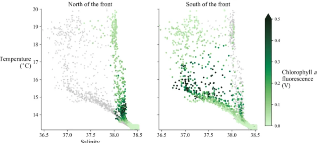
The distinct water properties on both sides of the front are evidenced by the T–S diagrams in Fig. 4, where the colours represent the fluorescence. The salinity range north of the front is roughly between 38 and 38.5, with the exception of a few measurements, and confirms the nature of the Mediter-ranean water mass. The fluorescence maximum appears be-tween 14 and 15◦C. South of the front, the salinity range is wider while the temperature values are similar to the north.
In addition to the CTDs, the R/V thermosalinograph continuously acquired temperature and conductivity along the ship track, from which near-surface salinity is derived (Fig. 5). The R/V weather station acquired air temperature, pressure, and wind speed and direction during the whole du-ration of the mission. Direct measurements of currents were performed with an acoustic Doppler current profiler and are presented in Sect. 3.5.
Figure 3.The CTD casts were organised into five legs that crossed the front and were repeated over two periods, at the beginning and the end of the mission.
3.1.1 Configuration
The CTD rosette was equipped with the following instru-ments:
– a Sea-Bird SBE 911Plus, two conductivity and temper-ature sensors, and one pressure sensor units;
– a SBE 43 oxygen sensor; and
– a Seapoint [FTU] fluorescence and turbidity sensor. The GEONICA METEODATA 2000 weather station mea-sured the following variables: air pressure, temperature, hu-midity, and wind speed and direction, with a resolution of 10 min. The continuous, near-surface measurements of tem-perature and salinity are provided by a SeaBird SBE21 ther-mosalinograph.
3.1.2 Quality control
The general checks described in Sect. 2.5.2 (i.e. ranges, spike, gradient and stationarity) are applied on the temper-ature, salinity, conductivity, and turbidity. The threshold val-ues are detailed in the corresponding tables in the QC pro-cedure document (SOCIB Data Center, 2018). As mentioned in Sect. 2.4, netCDF files with a correction applied on the salinity and conductivity are also provided (L1_corr). 3.2 Gliders
To collect measurements addressing the sub-mesoscale, two gliders were deployed on 25 May inside the study area. The
Figure 4.The T–S diagrams are shown separately for the casts located north and south of the front (broad, dashed line).
Figure 5.The near-surface salinity (coloured dots) measured by the thermosalinograph is evidence of strong horizontal gradients, in agree-ment with the front position, as obtained using the SST (broad, dashed line). The five subplots depict the temperature and salinity along selected meridional tracks.
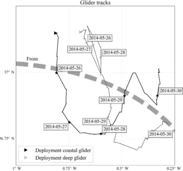
coastal glider carried out measurements up to a 200 m depth and the deep glider up to 500 m. The horizontal resolution was about 0.5 km for the shallow glider and 1 km for the deep glider. The initial sampling strategy consisted of two 50 km long, meridional tracks, 10 km away from each other, and to repeat these tracks up to 4 times during the experiment. However, due to the strong zonal currents in the frontal zone, different tracks (Fig. 6) crossing the front several times were made instead.
On 25 May at 19:24 (UTC), the deep glider payload suf-fered an issue with the data-logging software, resulting in no
data acquisition during a few hours, during which the prob-lem was being fixed. After this event, the data acquisition could be resumed on 26 May at 08:50 (UTC).
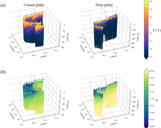
The mean vertical separation between two consecutive measurements is around 16 cm. Figure 7 displays the tem-perature and salinity sections obtained with the two vehicles. The high density of measurements makes it possible to dis-tinguish small-scale features on both sides of the front, such as strong lateral gradients, subduction, or filament structures. The gliders follow a 3-dimensional trajectory in the water column, but for some specific usages it is sometimes more
Figure 6.Deployment positions and trajectories of the gliders. Dif-ferent time instances separated by 1 day are indicated on the tracks to provide a temporal dimension.
convenient to have the glider data as if they were a series of vertical profiles. To do so, a binning is applied to the original data, leading to the L2 data, as described in Sect. 2.4. 3.2.1 Configuration
The information concerning the two gliders is summarised in Table 3. Due to safety concerns, both the deep and coastal gliders had their surfacing limited: the deep glider came to the surface one in every three profiles, while the coastal glid-ers came out one in every 10 profiles. While this strategy does not appear optimal from a scientific point of view (loss of measurements near the surface, meaning of the depth-averaged currents), the priority was set on the glider integrity. 3.2.2 Quality control
Before deployment, the glider compass was calibrated fol-lowing Merckelbach et al. (2008). The thermal-lag happen-ing on the unpumped Sea-Bird CTD sensors installed on the deep and coastal gliders was corrected using the procedure described in Garau et al. (2011).
The checks not yet applied but planned for the next release of the Glider toolbox include the removal of N aN values; the detection of impossible dates or locations; valid ranges (de-pending on depth) for the variables, spikes, and gradients; and constant values over a large range of depths in the pro-files. The tests performed that showed a constant value check proved useful for conductivity (and hence density and salin-ity). A new version of the present dataset will be released once these new checks are made operational.
Finally, oxygen concentration measurements (not shown here) seem to exhibit a lag. According to Bittig et al. (2014), this issue is also related to the time response of oxygen op-todes. As far as we know, there is not yet an agreement from the community on how to correct this lag, this is why the data are kept as they are in the present version, though we do not discard the possibility that an improvement in the glider toolbox could address this specific issue.
3.3 Surface drifters
On 25 May, 25 Surface Velocity Program (SVP, Lumpkin and Pazos, 2007) drifters were deployed in the frontal area in a tight square pattern, with a mean distance between neigh-bour drifters of around 3 km. In the Mediterranean Sea, they have been shown to provide information on surface dynam-ics, ranging from basin scale to mesoscale features or coastal currents (Poulain et al., 2013). Almost all the drifters were equipped with a thermistor on the lower part of the buoy to measure sea water temperature.
A total of 11 out the 25 drifters, especially those deployed more to the south, were captured by the intense Algerian Cur-rent and followed a trajectory along the coast to a longitude about 5◦300E. The other drifters were deflected northward when they reached about 0◦300E, then veered northwestward or eastward and described cyclonic and anticyclonic trajecto-ries, respectively. All the drifters moved along the front po-sition (deduced from the SST images), until they encounter the Algerian Current (Fig. 8).
On average, the temporal sampling resolution is close to 1 h, except for two drifters for which the intervals are 4 and 5 h. The velocities are directly computed from the successive positions and highlight the strength of the Algerian Current with velocities in the order of 1 m s−1(Fig. 9).
3.3.1 Configuration
The drifters deployed during the experiment are the World Ocean Circulation Experiment SVP mini-drifters. These drifters are made up of a surface buoy that includes a trans-mitter to relay data and a thermistor to measure the water temperature near the surface; the buoy is tethered to a holey-sock drogue centred at 15 m depth. The possible loss of the drogue is controlled with a tension sensor located below the surface buoy.
A total of 15 drifters were manufactured by Pacific Gyre and 10 by Data Buoy instrumentation (DBi). All the drifters contributed to the Mediterranean Surface Velocity Programme (MedSVP).
3.3.2 Quality control
Tests are applied on the position (i.e. on land), velocity and temperature records (valid ranges and spikes). Checking the platform speed is particularly relevant, as abnormally high
Figure 7.Temperature (a) and salinity (b) measured by the two gliders. The approximate front position at the surface is shown as a dashed grey line.
Table 3.Characteristics of the gliders.
Coastal glider Deep glider
Manufacturer Teledyne Webb Research Corp. Teledyne Webb Research Corp. Model Slocum, G1, shallow version (200 m) Slocum G1 Deep
Battery technology Alkaline C-cell Alkaline C-cell
Software version 7.13 (navigation), 3.17 (science) 7.13 (navigation), 3.17 (science)
On-board sensors CTD (S.B.E.) CTD (S.B.E.)
Oxygen: OPTODE 3835 (Aandera) Oxygen: OPTODE 3830 (Aandera)
Fluorescence–turbidity: FLNTUSLO (WetLabs) Fluorescence–turbidity: FLNTUSLK (WetLabs)
Number of casts 160 392
Total distance (km) 127 118
Max. depth (m) 200 500
values are intermittently encountered. See the SOCIB Data Center (2018) for the threshold values used in the checks. In addition, the method developed by Rio (2012) is used to improve the accuracy of the drogue presence from wind slip-page (Menna et al., 2018).
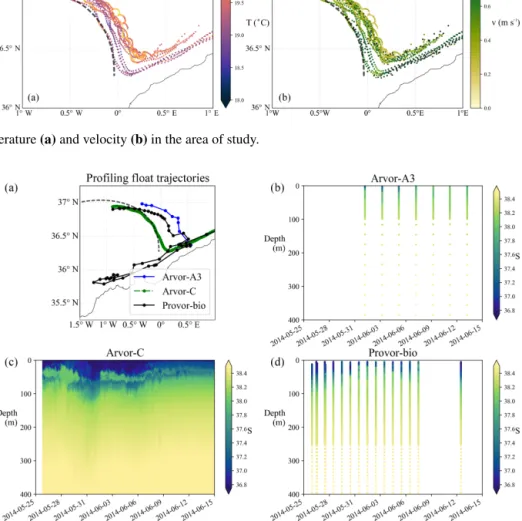
3.4 Profiling floats
Three profiling floats were deployed in the same zone as the drifters on 2 May (see Table 4). Their configuration depends on the float type: the Arvor-C has higher temporal resolution (hours) and does not go much deeper than 400 m. The A3 and Provor-bio platforms are usually set to have a cycle length
between 1 and 5 days, with the Provor-bio platform reaching maximal depth in the order of 1000 m. The floats constitute an essential tool in order to monitor the mesoscale (Sánchez-Román et al., 2017). The trajectories (Fig. 10) clearly show that profiles were acquired in the frontal area, before the floats were eventually captured by the Algerian Current.
The Arvor-C trajectory closely follows the front position until a latitude of 36◦300N, accounting for 455 profiles in the vicinity of the front. This is probably due to its configuration: its high frequency temporal sampling makes it possible to spend more time in the near-surface layer and hence the float follows the front better than the two other float types. Its last
Figure 8.Surface drifter trajectories. For the sake of simplicity and clarity, the temperature, when available, is only shown for the dura-tion of the AlborEx mission (25–31 May 2014).
profile was taken on 14 June 2014, at an approximate location of 36◦150N, 4◦E, then it drifted at the surface.
3.4.1 Configuration
The three floats provided temperature and salinity profiles thanks to the Sea-Bird CTD. In addition to these variables, the PROVBIO (PROVOR CTS4) platform measured bio-chemical and optical properties: coloured dissolved organic matter (CDOM), chlorophyll a concentration, backscatter-ing (650 nm), dissolved oxygen concentration and down-welling irradiance (380, 410, 490 nm), and photosyntheti-cally active radiation (PAR). Table 4 reports the main deploy-ment characteristics. All the floats are manufactured by NKE (Hennebont, France). The profiles were performed around noon, local time, and were used in combination with the glider measurements to study the deep chlorophyll maximum (DCM) across the front (Olita et al., 2017).
3.5 Current profiler
The Vessel Mounted-Acoustic Doppler Current Meter Pro-filer (VM-ADCP) acquired velocity profiles approximately every 2 min during night-time (22:00–06:00 UTC) at a speed of 10 knots and during the CTD surveys (see Fig. 3). The measurement accuracy is in the order of 0.01 m s−1. The measurements were vertically averaged over 8 m depth bins. The velocities exhibit a dominant eastward current with speed locally larger than 1 m s−1and a signal that is clearly visible in the first 100 m of the water column. The velocity field is illustrated in Fig. 11, where each velocity vector is shown as a bar with a colour depending on the intensity. The vertical structure is also displayed along with the front posi-tion.
3.5.1 Configuration
The current profiler is an Ocean Surveyor ADCP, manufac-tured by Teledyne RD Instruments and operating at a fre-quency of 150 kHz. This instrument was configured with 8 m depth bins and a total of 50 bins. Final velocity profiles were averaged in 10 min intervals. The transducer depth is approx-imately 2 m.
The position and behaviour (heading, pitch, and roll) of the research vessel is obtained with an Ashtec 3-D GPS 800 ADU positioning system that provides provide geographical positions with a 10–20 cm accuracy and heading, pitch, and roll with an accuracy on the order of 1◦. The instrument was calibrated to correct the misalignment angle and scaling fac-tor. The technical report referring to this platform is available in Annex II of Ruiz et al. (2015).
3.5.2 Quality checks
The vessel’s velocity is 1 or 2 orders of magnitudes greater than the currents that have to be measured, hence this type of current measurements requires a careful processing in or-der to get meaningful velocities from the raw signal. The QC procedure for the VM-ADCP is complex as it involves tests on more than 40 technical and geophysical variables (SO-CIB Data Center, 2018). The different tests are based on the technical reports of Cowley et al. (2009) and Bender and Di-Marco (2009), which are aimed primarily at ADCP mounted on moorings. The procedure can be summarised as follows.
1. Technical variables. Valid ranges are checked for each of these variables: if the measurement is outside the range, the QF is set to 4 (bad data). Examples of tech-nical variables are bottom track depth, sea water noise amplitude, and correlation magnitude.
2. Vessel behaviour. Vessel pitch, roll, and orientation an-gles are checked and QF are assigned based on specific ranges. In addition, the vessel velocity is checked and anomalously high values are also flagged as bad. 3. Velocities. Valid ranges are provided for the computed
current velocities: up to 2 m s−1, velocities are consid-ered as good; between 2 and 3 m s−1, probably good, and above 3 m s−1, bad.
The application of all of these tests led to Fig 12, which illustrates the QF during the whole mission. The three main periods during which the ADCP was turned off are shown as grey areas. In addition, no measurements are available in the first metres of the water column, due to the position of the ADCP on the ship, at a depth of approximately 2 m.
Overall, the quality of the data tends to deteriorate when the depth increases, as reflected by the bad and missing val-ues. In the first 200 m, about 95 % of the measurements are considered as good. Below 200 m, the ratio drops to 57 % with more than 21 % of missing values. Note that the flags 5, 7 and 8 were not used in this case but kept in the plot.
Figure 9.Drifter temperature (a) and velocity (b) in the area of study.
Figure 10.Profiling float trajectories and salinity from 25 May to 15 June 2014.
3.6 Nutrients
Samples for nutrient analysis were collected in triplicate from CTD Niskin bottles and immediately frozen for sub-sequent analysis at the laboratory. Concentrations of dis-solved nutrients (Nitrite: NO−2, Nitrate: NO−3, and Phos-phate: PO3−4 ) were determined with an autoanalyser (Al-liance Futura) using colourimetric techniques (Grasshoff et al., 1983). The accuracy of the analysis was established using the Coastal Seawater Reference Material for Nutri-ents (MOOS-1, NRCCNRC), resulting in recoveries of 97 %, 95 %, and 100 % for NO−2, NO−3, and PO3−4 , respectively. Detection limits were NO−2: 0.005 µM, NO−3: 0.1 µM, and PO3−4 : 0.1 µM.
4 Description of the database
The AlborEx mission generated a large amount of data in a region sparsely sampled in the past. The synergy between low-resolution (CTD, drifters, floats) and high-resolution data (ADCP, gliders) makes this dataset unique for the study of sub-mesoscale processes in the Mediterranean Sea. More-over its multidisciplinary nature makes it suitable to study the interactions between the physical conditions and the bio-geochemical variables.
4.1 File format and organisation
The original data files (i.e. obtained directly from the sensors and with a format depending on the manufac-turer) are converted to the Network Common Data Form (netCDF, https://doi.org/http://doi.org/10.5065/D6H70CW6, last access: 3 August 2018), an Open Geospatial Consortium
Table 4.Characteristics of the profiling floats.
Platform Final date Maximal depth Cycle length No. of profiles
(m) Mission Total
ARVOR-A3 17 Jun 2014 2000 1 day 3 12
ARVOR-C 17 Jun 2014 400 1.5 h 144 2507
PROVOR CTS4 24 Apr 2015 1000 1 day until 7 Jun, 9 71 then 5 days
Figure 11.Velocity field obtained with the ADCP at a 40 m depth (a) and sections of zonal velocity on 26 May (S1, b) and 27 May (S2, c). The locations of the sections are indicated by dashed rectangles on the map. Only data with a quality flag equal to 1 (good data) are represented.
(OGC) standard widely adopted in atmospheric and oceanic sciences. Each file contains the measurements acquired by the sensors as well the metadata (mission name, principal in-vestigator, etc.). The structure of the files follows the Climate and Forecast (CF) conventions (Domenico and Nativi, 2013) and are based on the model of OceanSITES (Send et al., 2010).
4.2 File naming
In order to keep the file names consistent with the original database, it was decided to keep the same file names as those assigned by the SOCIB Data Cen-ter. As an example, we deconstruct one file name – dep0007_socib-rv_scb-sbe9002_L1_2014-05 -25– into its different parts below.
dep0007 indicates the number of the deployment, where deployment is the equivalent to the start of a mission or survey with a given platform. The deployment ends
when the mission is over or if the platform stops acquir-ing data.
socib-rv is the code for the platform, in this case the SOCIBcoastal research vessel.
scb-sbe9002 is the instrument identifier, here the CTD SeaBird 9Plus. Note that the instrument is described in the metadata of the netCDF file.
L1 is the processing level (see Sect. 2.4).
2014-05-25 is the deployment date (year-month-day). Now the general naming is defined, Table 5 lists the differ-ent files made available in the dataset.
4.3 Data reading and visualisation
The standard format (netCDF) in which the data files are written makes the reading and visualisation straightforward. A variety of software tools such as ncview, ncBrowse,
Figure 12.Quality flags for the velocity measurements. The areas marked with a × are those during which the VM-ADCP was not acquiring measurements.
Table 5.Platform corresponding to the different files.
File name Platform
dep0023_socib-rv_scb-rdi001_L1_2014-05.nc ADCP
dep0007_socib-rv_scb-sbe9002_L1_2014-05-25.nc CTD
dep0001_drifter-svp***_scb-svp***_L1_2014-05-25.nc SVP drifters (×25)
dep0005_icoast00_ime-slcost000_L1_2014-05-25_data_dt.nc Coastal glider
dep0012_ideep00_ime-sldeep000_L1_2014-05-25_data_dt.nc Deep glider
dep0001_profiler-drifter-arvora3001_ogs-arvora3001_L1_2014-05-25.nc Arvor-A3 float
dep0001_profiler-drifter-arvorc_socib_arvorc_L1_2014-05-25.nc Arvor-C float
dep0001_profiler-drifter-provbioll001_ogs-provbioll001_L1_2014-05-25.nc Provor-Bio float
dep0015_socib-rv_scb-met009_L1_2014-05-25.nc Weather onboard R/V
dep0015_socib-rv_scb-pos001_L1_2014-05-25.nc Navigation data from R/V
dep0015_socib-rv_scb-tsl001_L1_2014-05-25.nc Thermosalinograph
dep0015_socib-rv_scb-tsl001_L1_2014-05-25_HR.nc Thermosalinograph (high-res.)
*** in the file names stands for 3 digits.
or Panoply are designed to visualise gridded fields. Here the data provided consist of trajectories (surface or 3-dimensional), profiles, and trajectory-profiles, which can be easily read using the netCDF library in different languages (Table 6).
Examples of reading and plotting functions, written in Python, are also provided (Troupin, 2018). They allow users or readers to get the data from the files and reproduce the same figures as in the paper, constituting a good starting point to carry out further specific analysis.
When accessing the data catalog, users are provided a list of in-house visualisation tools designed to offer quick visu-alisation of the file content. The visuvisu-alisation tools depend on the type of data: JWebChart is used for time series; Dapp displays the trajectory of a moving platform on a map; the profile-viewer allows the user to select locations on the map and view the corresponding profiles.
5 Code and data availability
Following SOCIB general policy, the data are made avail-able as netCDF files through the SOCIB Thematic Real-time Environmental Distributed Data Services (THREDDS) data server, a standard way to distribute metadata and data us-ing a variety of remote data access protocols such as OPeN-DAP, Web Map Service (WMS), or direct HTTP access. In addition, the whole AlborEx dataset has been assigned a digital object identifier (DOI) to make it uniquely citable. The most recent version of the dataset is accessible from http://doi.org/10.25704/z5y2-qpye (last access: 24 Decem-ber 2018; Pascual et al., 2018), and the nutrient data, in the process of being included in the catalog, are available at https://doi.org/10.5281/zenodo.2384855 (last access: 24 De-cember 2018; Troupin, 2018).
Upgrades will be performed periodically with the imple-mentation of fresh or better QCs on sensors such as the ADCP, CTD, or gliders. The new releases will be available using the same Zenodo identifier, but will be assigned a
dif-Table 6.NetCDF libraries for various languages.
Programming language Library
Python https://github.com/Unidata/netcdf4-python (last access: 24 December 2018) Fortran https://github.com/Unidata/netcdf-fortran(last access: 24 December 2018) C https://github.com/Unidata/netcdf-c(last access: 24 December 2018) Javascript https://www.npmjs.com/package/netcdf4(last access: 24 December 2018) Octave https://github.com/Alexander-Barth/octave-netcdf(last access: 24 December 2018) Julia https://github.com/Alexander-Barth/NCDatasets.jl(last access: 24 December 2018) MATLAB Native support since version R2010b
ferent version number, each version having its own DOI. Files not available at the time of the writing will also be ap-pended to the original database.
Concerning the improvement of the quality control, it is worth mentioning the new tests that will be implemented in the SOCIB Glider Toolbox (Troupin et al., 2016).
The checks performed on the ADCP velocities involve a set of parameters that can also be fine-tuned to improve the relevance of the quality flags. Nevertheless, noticeable changes are not expected with respect to the quality flags dis-played in Fig. 12.
Finally, the quality of the CTD and the glider profiles can be improved by using the salinity measurements of water samples collected during the mission. This type of correction might not be essential for the study of mesoscale processes but is crucial when one is focused on long-term studies and when a drift can be observed in the salinity measurements.
A set of programs in Python to read the files and represent their content, as in the figures presented through the paper, are available at https://github.com/ctroupin/AlborEX-Data (last access: 24 December 2018). The programs are writ-ten in the form of documented Jupyter notebooks, a web ap-plication that combines code fragments, equations, graphics, and explanatory text (http://jupyter.org/, last access: 14 Au-gust 2018), so that they can be run step by step. The fig-ure’s colourmaps were produced using the cmocean mod-ule (Thyng et al., 2016).
6 Conclusions and perspectives
The AlborEx observations acquired in May 2014 consti-tute a unique observational dataset that captured mesoscale and sub-mesoscale features in a particularly energetic frontal zone in the western Mediterranean Sea. The potential uses of the dataset can be separated into the following different topics.
– Hydrodynamic model validation. With their increasing resolution, models are becoming able to properly repro-duce small-scale structures, but the correct timing and location of these features remain a challenging topic.
– resolution remote-sensing data validation. High-quality in situ measurements of the sea surface are es-sential for the validation of operational products such SST or Ocean Color.
– Study of mechanisms. The Mediterranean Sea is often referred to as a laboratory for oceanography and the Alboran Sea in particular is a stage for intense processes of mixing, subduction, and instability.
– Assessment of mechanisms responsible for intense ver-tical motions.
The version of the dataset described in the present paper contains files that have been processed and standardised so that they are directly usable by scientists without having to perform unit or format conversions from the manufacturer’s raw data files.
Updates will be performed when new files or new versions of the existing files are made available.
Author contributions. CT prepared the figures and the first ver-sion of the manuscript. AP and SR edited the manuscript. JGF and MAR lead the data management and the creation of a DOI in Datacite. CM implemented the processing of the ADCP data. GN helped with the processing of the drifters and profiling floats. EA and AT processed and provided the biochemical data. IR finalised the QC documentation.
Competing interests. The authors declare that the research was conducted in the absence of any commercial or financial relation-ships that could be construed as a potential conflict of interest.
Disclaimer. The authors do not accept any liability for the correct-ness and appropriate interpretation of the data or their suitability for any use.
Acknowledgements. We wish to thank the three anonymous reviewers for their constructive comments and the extensive check of the data files. AlborEx was conducted in the framework of PERSEUS EU-funded project (grant agreement no. 287600).
Glider operations were partially funded by the JERICO FP7 project. Ananda Pascual acknowledges support from the Spanish National Research Program (E-MOTION/CTM2012-31014 and PRE-SWOT/CTM2016-78607-P). Simon Ruiz and Ananda Pas-cual are also supported by the Copernicus Marine Environment Monitoring Service (CMEMS) MedSUB project. Antonio Olita was supported by the JERICO-TNA program, through the FRIPP (FRontal Dynamics Influencing Primary Production) project. The profiling floats and some drifters were contributed by the Argo-Italy program. The proceedings of such an ambitious mission would not have been possible without the involvement of numerous staff both at sea and on land: Ana Massanet, Margarita Palmer, Irene Lizaran, Carlos Castilla, Pau Balaguer, Milena Menna, Kristian Sebastián, Sebastián Lora, and Antonio Bussani.
Edited by: Giuseppe M. R. Manzella Reviewed by: three anonymous referees
References
Adloff, F., Somot, S., Sevault, F., Jordà, G., Aznar, R., Déqué, M., Herrmann, M., Marcos, M., Dubois, C., Padorno, E., Alvarez-Fanjul, E., and Gomis, D.: Mediterranean Sea response to cli-mate change in an ensemble of twenty first century scenarios, Clim. Dynam., 45, 2775–2802, https://doi.org/10.1007/s00382-015-2507-3, 2015.
Alvarez, A., Tintoré, J., and Sabatés, A.: Flow modification and shelf-slope exchange induced by a submarine canyon off the northeast Spanish coast, J. Geophys. Res.-Oceans, 101, 12043– 12055, https://doi.org/10.1029/95jc03554, 1996.
Aulicino, G., Cotroneo, Y., Ruiz, S., Sánchez Román, A., Pascual, A., Fusco, G., Tintoré, J., and Budillon, G.: Monitoring the Alge-rian Basin through glider observations, satellite altimetry and nu-merical simulations along a SARAL/AltiKa track, J. Mar. Syst., 179, 55–71, https://doi.org/10.1016/j.jmarsys.2017.11.006, 2018.
Bender, L. and DiMarco, S.: Quality Control and Analysis of Acoustic Doppler Current Profiler Data Collected on Offshore Platforms of the Gulf of Mexico, Tech. rep., U.S. Dept. of the Interior, Minerals Mgmt. Service, Gulf of Mexico OCS Region, New Orleans, LA, 66 pp., 2009.
Bergamasco, A. and Malanotte-Rizzoli, P.: The circulation of the Mediterranean Sea: a historical review of experi-mental investigations, Adv. Oceanogr. Limnol., 1, 11–28, https://doi.org/10.1080/19475721.2010.491656, 2010.
Berta, M., Bellomo, L., Griffa, A., Magaldi, M. G., Molcard, A., Mantovani, C., Gasparini, G. P., Marmain, J., Vetrano, A., Béguery, L., Borghini, M., Barbin, Y., Gaggelli, J., and Quentin, C.: Wind-induced variability in the Northern Current (northwest-ern Mediterranean Sea) as depicted by a multi-platform observ-ing system, Ocean Sci., 14, 689–710, https://doi.org/10.5194/os-14-689-2018, 2018.
Bittig, H. C., Fiedler, B., Scholz, R., Krahmann, G., and Körtzinger, A.: Time response of oxygen optodes on pro-filing platforms and its dependence on flow speed and temperature, Limnol. Oceanogr. Methods, 12, 617–636, https://doi.org/10.4319/lom.2014.12.617, 2014.
Bonaduce, A., Pinardi, N., Oddo, P., Spada, G., and Larni-col, G.: Sea-level variability in the Mediterranean Sea from
altimetry and tide gauges, Clim. Dynam., 47, 2851–2866, https://doi.org/10.1007/s00382-016-3001-2, 2016.
Bosse, A., Testor, P., Mortier, L., Prieur, L., Taillandier, V., d’Ortenzio, F., and Coppola, L.: Spreading of Lev-antine Intermediate Waters by submesoscale coherent vor-tices in the northwestern Mediterranean Sea as observed with gliders, J. Geophys. Res.-Oceans, 120, 1599–1622, https://doi.org/10.1002/2014jc010263, 2015.
Bouffard, J., Pascual, A., Ruiz, S., Faugère, Y., and Tintoré, J.: Coastal and mesoscale dynamics characterization using altime-try and gliders: A case study in the Balearic Sea, J. Geophys. Res., 115, C10029, https://doi.org/10.1029/2009jc006087, 2010. Cheney, R. E.: Recent observations of the Alboran Sea frontal system, J. Geophys. Res., 83, 4593, https://doi.org/10.1029/jc083ic09p04593, 1978.
Cotroneo, Y., Aulicino, G., Ruiz, S., Pascual, A., Budillon, G., Fusco, G., and Tintoré, J.: Glider and satellite high resolution monitoring of a mesoscale eddy in the algerian basin: Effects on the mixed layer depth and biochemistry, J. Mar. Syst., 162, 73– 88, https://doi.org/10.1016/j.jmarsys.2015.12.004, 2016. Cowley, R., Heaney, B., Wijffels, S., Pender, L., Sprintall, J.,
Kawamoto, S., and Molcard, R.: INSTANT Sunda Data Report Description and Quality Control, Tech. rep., CSIRO, 2009. Crise, A., Ribera d’Alcalà, M., Mariani, P., Petihakis, G., Robidart,
J., Iudicone, D., Bachmayer, R., and Malfatti, F.: A Conceptual Framework for Developing the Next Generation of Marine OB-servatories (MOBs) for Science and Society, Front. Mar. Sci., 5, 1–8, https://doi.org/10.3389/fmars.2018.00318, 2018.
Damien, P., Bosse, A., Testor, P., Marsaleix, P., and Estournel, C.: Modeling Postconvective Submesoscale Coherent Vortices in the Northwestern Mediterranean Sea, J. Geophys. Res.-Oceans, 122, 9937–9961, https://doi.org/10.1002/2016jc012114, 2017. Delaney, J. R. and Barga, R. S.: Observing the Oceans – A 2020
Vision for Ocean Science, 27–38, Microsoft Research, avail-able at: https://www.microsoft.com/en-us/research/publication/ observing-the-oceans-a-2020-vision-for-ocean-science/ (last access: 31 August 2018), 2009.
Domenico, B. and Nativi, S.: CF-netCDF3 Data Model Exten-sion standard, Tech. Rep. OGC 11-165r2, Open Geospatial Consortium, available at: https://portal.opengeospatial.org/files/ ?artifact_id=51908 (last access: 31 August 2018), 2013. Garau, B., Ruiz, S., Zhang, W. G., Pascual, A., Heslop, E.,
Ker-foot, J., and Tintoré, J.: Thermal Lag Correction on Slocum CTD Glider Data, J. Atmos. Ocean. Technol., 28, 1065–1071, https://doi.org/10.1175/jtech-d-10-05030.1, 2011.
Giorgi, F.: Climate change hot-spots, Geophys. Res. Lett., 33, L08707, https://doi.org/10.1029/2006gl025734, 2006.
Giorgi, F. and Lionello, P.: Climate change projections for the Mediterranean region, Global Planet. Change, 63, 90–104, https://doi.org/10.1016/j.gloplacha.2007.09.005, 2008.
Grasshoff, K., Kremling, K., and Ehrhardt, M. (Eds.): Methods of Seawater Analysis, Verlag Chemie GmbH, 2nd rev. and extended edn., https://doi.org/10.1002/9783527613984, 419 p., 1983. Guiot, J. and Cramer, W.: Climate change: The 2015 Paris
Agree-ment thresholds and Mediterranean basin ecosystems, Science, 354, 465–468, https://doi.org/10.1126/science.aah5015, 2016. Hernandez-Lasheras, J. and Mourre, B.: Dense CTD survey versus
in a regional ocean model west of Sardinia, Ocean Sci., 14, 1069– 1084, https://doi.org/10.5194/os-14-1069-2018, 2018.
Iona, A., Theodorou, A., Sofianos, S., Watelet, S., Troupin, C., and Beckers, J.-M.: Mediterranean Sea climatic indices: mon-itoring long-term variability and climate changes, Earth Syst. Sci. Data, 10, 1829–1842, https://doi.org/10.5194/essd-10-1829-2018, 2018a.
Iona, A., Theodorou, A., Watelet, S., Troupin, C., Beckers, J.-M., and Simoncelli, S.: Mediterranean Sea Hydrographic At-las: towards optimal data analysis by including time-dependent statistical parameters, Earth Syst. Sci. Data, 10, 1281–1300, https://doi.org/10.5194/essd-10-1281-2018, 2018b.
Johnston, T. M. S., Rudnick, D. L., Tintoré, J., and Wirth, N.: Co-herent Lagrangian Pathways from the Surface Ocean to Interior (CALYPSO): Pilot Cruise report, Tech. rep., Scripps Institution of Oceanography (SIO), available at: http://scrippsscholars.ucsd. edu/tmsjohnston/files/calypssocibcruisereport2018.pdf, last ac-cess: 17 December 2018.
Lumpkin, R. and Pazos, M.: Measuring surface currents with Surface Velocity Program drifters: the instrument, its data, and some recent results, in: Lagrangian Analysis and Pre-diction of Coastal and Ocean Dynamics, edited by: Griffa, A., Kirwan Jr., A. D., Mariano, A. J., Özgökmen, T., and Rossby, H. T., 39–67, Cambridge University Press, https://doi.org/10.1017/CBO9780511535901.003, 2007. Macias, D., Garcia-Gorriz, E., and Stips, A.: Deep winter
con-vection and phytoplankton dynamics in the NW Mediterranean Sea under present climate and future (horizon 2030) scenarios, Sci. Rep., 8, 1–15, https://doi.org/10.1038/s41598-018-24965-0, 2018.
Margirier, F., Bosse, A., Testor, P., L’Hévéder, B., Mortier, L., and Smeed, D.: Characterization of Convective Plumes As-sociated With Oceanic Deep Convection in the Northwest-ern Mediterranean From High-Resolution In Situ Data Col-lected by Gliders, J. Geophys. Res.-Oceans, 122, 9814–826, https://doi.org/10.1002/2016JC012633, 2017.
MEDOC-Group, T.: Observation of Formation of Deep Water in the Mediterranean Sea, 1969, Nature, 225, 1037–1040, https://doi.org/10.1038/2271037a0, 1970.
Melet, A., Verron, J., and Brankart, J.-M.: Potential outcomes of glider data assimilation in the Solomon Sea: Control of the water mass properties and parameter estimation, J. Mar. Syst., 94, 232– 246, https://doi.org/10.1016/j.jmarsys.2011.12.003, 2012. Menna, M., Poulain, P.-M., Bussani, A., and Gerin, R.:
De-tecting the drogue presence of SVP drifters from wind slip-page in the Mediterranean Sea, Measurement, 125, 447–453, https://doi.org/10.1016/j.measurement.2018.05.022, 2018. Merckelbach, L., Briggs, R., Smeed, D., and Griffiths, G.: Current
measurements from autonomous underwater gliders, in: 2008 IEEE/OES 9th Working Conference on Current Measurement Technology, IEEE, https://doi.org/10.1109/ccm.2008.4480845, 2008.
Millot, C.: Circulation in the Western Mediterranean Sea, Oceanol. Acta, 10, 143–148, 1987.
Millot, C.: Mesoscale and seasonal variabilities of the circulation in the western Mediterranean, Dynam. Atmos. Oceans, 15, 179– 214, https://doi.org/10.1016/0377-0265(91)90020-G, 1991.
Millot, C.: Circulation in the Western Mediterranean Sea, J. Mar. Syst., 20, 423–442, https://doi.org/10.1016/S0924-7963(98)00078-5, 1999.
Mourre, B. and Chiggiato, J.: A comparison of the performance of the 3-D super-ensemble and an ensemble Kalman filter for short-range regional ocean prediction, Tellus A, 66, 21640, https://doi.org/10.3402/tellusa.v66.21640, 2014.
Olita, A., Capet, A., Claret, M., Mahadevan, A., Poulain, P. M., Ribotti, A., Ruiz, S., Tintoré, J., Tovar-Sánchez, A., and Pas-cual, A.: Frontal dynamics boost primary production in the sum-mer stratified Mediterranean Sea, Ocean Dynam., 67, 767–782, https://doi.org/10.1007/s10236-017-1058-z, 2017.
Pan, C., Zheng, L., Weisberg, R. H., Liu, Y., and Lembke, C. E.: Comparisons of different ensemble schemes for glider data as-similation on West Florida Shelf, Ocean Modell., 81, 13–24, https://doi.org/10.1016/j.ocemod.2014.06.005, 2014.
Pascual, A., Ruiz, S., Olita, A., Troupin, C., Claret, M., Casas, B., Mourre, B., Poulain, P.-M., Tovar-Sanchez, A., Capet, A., Mason, E., Allen, J., Mahadevan, A., and Tintoré, J.: A mul-tiplatform experiment to unravel meso- and submesoscale pro-cesses in an intense front (AlborEx), Front. Mar. Sci., 4, 3, https://doi.org/10.3389/fmars.2017.00039, 2017.
Pascual, A., Ruiz, S., Troupin, C., Olita, A., Casas, B., Margirier, F., Poulain, P.-M., Torner, M., Fernández, J. G., Rújula, M. À., Muñoz, C., Notario, X., Ruíz, I., Roque, D., Tovar, A., Allen, J. T., and Tintoré, J.: ALBOREX 2014 – PERSEUS (Version 1.0) [Data set], Balearic Islands Coastal Observing and Forecasting System, SOCIB, https://doi.org/10.25704/Z5Y2-QPYE, 2018. Pinot, J.-M., Tintoré, J., and Gomis, D.: Multivariate analysis of
the surface circulation in the Balearic Sea, Prog. Oceanogr., 36, 343–376, https://doi.org/10.1016/0079-6611(96)00003-1, 1995. Poulain, P.-M., Bussani, A., Gerin, R., Jungwirth, R.,
Mauri, E., Menna, M., and Notarstefano, G.: Mediter-ranean Surface Currents Measured with Drifters: From Basin to Subinertial Scales, Oceanography, 26, 38–47, https://doi.org/10.5670/oceanog.2013.03, 2013.
Pujol, M.-I. and Larnicol, G.: Mediterranean sea eddy kinetic en-ergy variability from 11 years of altimetric data, J. Mar. Syst., 58, 121–142, https://doi.org/10.1016/j.jmarsys.2005.07.005, 2005. Rahmstorf, S.: Influence of mediterranean outflow on climate,
Eos, Transactions American Geophysical Union, 79, 281–281, https://doi.org/10.1029/98eo00208, 1998.
Rio, M.-H.: Use of Altimeter and Wind Data to Detect the Anoma-lous Loss of SVP-Type Drifter’s Drogue, J. Atmos. Ocean. Tech-nol., 29, 1663–1674, https://doi.org/10.1175/jtech-d-12-00008.1, 2012.
Robinson, A., Leslie, W., Theocharis, A., and Las-caratos, A.: Mediterranean Sea Circulation, in: En-cyclopedia of Ocean Sciences, 1689–1705, Elsevier, https://doi.org/10.1006/rwos.2001.0376, 2001.
Ruiz, S., Pascual, A., Casas, B., Poulain, P., Olita, A., Troupin, C., Torner, M., Allen, J., Tovar, A., Mourre, B., Massanet, A., Palmer, M., Margirier, F., Balaguer, P., Castilla, C., Claret, M., Mahadevan, A., and Tintoré, J.: Report on operation and data analysis from multiplatform synoptic intensive experiment (Al-borEx), Tech. rep., D3.8 Policy-oriented marine Environmental Research in the Southern European Seas, 120 pp., 2015. Sánchez-Román, A., Ruiz, S., Pascual, A., Mourre, B., and
floats in the Mediterranean Sea, Ocean Sci., 13, 223–234, https://doi.org/10.5194/os-13-223-2017, 2017.
Send, U., Font, J., Krahmann, G., Millot, C., Rhein, M., and Tin-toré, J.: Recent advances in observing the physical oceanography of the western Mediterranean Sea, Prog. Oceanogr., 44, 37–64, https://doi.org/10.1016/s0079-6611(99)00020-8, 1999.
Send, U., Weller, R. A., Wallace, D., Chavez, F., Lampitt, R. L., Dickey, T., Honda, M., Nittis, K., Lukas, R., McPhaden, M., and Feely, R.: OceanSITES, Proceedings of OceanObs’09: Sustained Ocean Observations and Information for Society, https://doi.org/10.5270/oceanobs09.cwp.79, 2010.
Simoncelli, S., Tonani, M., Grandi, A., Coatanoan, C., Myroshny-chenko, V., Sagen, H., Bäck, O., Scory, S., Schlitzer, R., and Fichaut, M.: First Release of the SeaDataNet Aggregated Data Sets Products. WP10 Second Year Report – DELIVERABLE D10.2., Tech. rep., SeaDataNet, https://doi.org/10.13155/49827, 2014.
Simoncelli, S., Grandi, A., , and Iona, S.: New Mediterranean Sea climatologies, in: IMDIS 2016 International Confer-ence on Marine Data and Information Systems, Vol. 57, 1–152, IOPAN and IMGW, Gdansk, Poland, available at: https://imdis.seadatanet.org/content/download/104127/1498227/ file/IMDIS2016_proceedings.pdf?version=1 (last access: 31 August 2018), 2016.
Skliris, N.: Past, Present and Future Patterns of the Thermo-haline Circulation and Characteristic Water Masses of the Mediterranean Sea, 29–48, Springer Netherlands, Dordrecht, https://doi.org/10.1007/978-94-007-6704-1_3, 2014.
SOCIB Data Center: SOCIB Quality Control Procedures, Tech. rep., Balearic Islands Coastal Observing and Forecasting Sys-tem, Palma de Mallorca, Spain, https://doi.org/10.25704/q4zs-tspv, 2018.
Stommel, H.: Deep winter convection in the western Mediterranean Sea, in: Studies in physical oceanography: A tribute to Georg Wüst on his 80th birthday, edited by: Gordon, A. L., Vol. 2, p. 232, Gordon and Breach Science, 1972.
Testor, P. and Gascard, J.-C.: Large-Scale Spread-ing of Deep Waters in the Western Mediterranean Sea by Submesoscale Coherent Eddies, J. Phys. Oceanogr., 33, 75–87, https://doi.org/10.1175/1520-0485(2003)033<0075:LSSODW>2.0.CO;2, 2003.
Testor, P., Bosse, A., Houpert, L. et al.: Multiscale Observations of Deep Convection in the Northwestern Mediterranean Sea During Winter 2012-2013 Using Multiple Platforms, J. Geophys. Res.-Oceans, 123, 1745–1776, https://doi.org/10.1002/2016jc012671, 2018.
Thyng, K., Greene, C., Hetland, R., Zimmerle, H., and DiMarco, S.: True Colors of Oceanography: Guidelines for Effective and Accurate Colormap Selection, Oceanography, 29, 9–13, https://doi.org/10.5670/oceanog.2016.66, 2016.
Tintoré, J., Gomis, D., Alonso, S., and Parrilla, G.: Mesoscale Dynamics and Vertical Motion in the Alborán Sea, J. Phys. Oceanogr., 21, 811–823, https://doi.org/10.1175/1520-0485(1991)021<0811:mdavmi>2.0.co;2, 1991.
Tintoré, J., Vizoso, G., Casas, B., Heslop, E., Pascual, A., Or-fila, A., Ruiz, S., Martínez-Ledesma, M., Torner, M., Cusí, S., and et al.: SOCIB: The Balearic Islands Coastal Ocean Observ-ing and ForecastObserv-ing System RespondObserv-ing to Science, Technol-ogy and Society Needs, Mar. Technol. Soc. J., 47, 101–117, https://doi.org/10.4031/mtsj.47.1.10, 2013.
Troupin, C.: AlborEx-Data-Python tools v1.0.0, Tech. rep., Univer-sity of Liège, https://doi.org/10.5281/zenodo.2384855, 2018. Troupin, C., Pascual, A., Valladeau, G., Pujol, I., Lana, A., Heslop,
E., Ruiz, S., Torner, M., Picot, N., and Tintoré, J.: Illustration of the emerging capabilities of SARAL/AltiKa in the coastal zone using a multi-platform approach, Adv. Space Res., 55, 51–59, https://doi.org/10.1016/j.asr.2014.09.011, 2015.
Troupin, C., Beltran, J., Heslop, E., Torner, M., Garau, B., Allen, J., Ruiz, S., and Tintoré, J.: A toolbox for glider data pro-cessing and management, Methods Oceanogr., 13-14, 13–23, https://doi.org/10.1016/j.mio.2016.01.001, 2016.
Tsimplis, M. N. and Rixen, M.: Sea level in the Mediterranean Sea: The contribution of temperature and salinity changes, Geophys. Res. Lett., 29, 51-1–51-4, https://doi.org/10.1029/2002gl015870, 2002.
Wolff, C., Vafeidis, A. T., Muis, S., Lincke, D., Satta, A., Lionello, P., Jimenez, J. A., Conte, D., and Hinkel, J.: A Mediterranean coastal database for assessing the impacts of sea-level rise and associated hazards, Sci. Data, 5, 180044, https://doi.org/10.1038/sdata.2018.44, 2018.
Wüst, G.: On the vertical circulation of the Mediter-ranean Sea, J. Geophys. Res., 66, 3261–3271, https://doi.org/10.1029/jz066i010p03261, 1961.