Welcome to migrants in a
borderless Europe
Bryophytes show the way to go
Alice Ledent, PhD student @ULiege
Introduction
sequently a substantial ice-dammed lake again formed in the basin during this advance (Busschers, 2008).
The Samarovo glacial maximum of West Siberia is considered to be of Saalian age. However, considering the scarcity of geological information from this region, a pre-Holsteinian glaciation may well have been the most extensive in eastern Central Siberia. During the glacial maximum all northward flowing rivers were blocked, and drainage of Siberia from as far east as Lake Baikal was redirected via the Aral Sea and Caspian Sea into the Black Sea and Mediterranean, multiplying its freshwater supply. Immediately west of the Urals, the position of the ice limits is still controversial. The Saalian limit was probably positioned in the Volga-Pechora interfluve area (Ehlers et al., 2004a).
At the end of the Saalian glacial maximum the ice in Denmark and North Germany possibly melted back beyond the southern Baltic Sea coast. Later readvances in Denmark and North Germany are probably the equivalents of the Warthe (Warta) Substage. Also, the Moscow Till of Russia is the equivalent of the Polish Warta Glaciation. Towards the east, its outer limit converges with that of the Older Saalian (Dnieper) glaciation, and it may even have advanced beyond the Dnieper glacial limit.
In the Alps, the classical Günz comprises several glaciations. Part of what has been originally refererd as Günz is Early Pleisto-cene, part is Middle Pleistocene. Between the Günzian and the Min-delian a separate Haslach Glaciation has been postulated, based on the occurrence of distinct gravel units south of Ulm (Schreiner, 1997). However, the scarcity of early Middle Pleistocene deposits and the lack of age control make it difficult to revise this part of the classical Alpine stratigraphy. Even the stratigraphy of the Alpine Rissian cold Stage is still far from solved—at least in major parts of the glaciated area. Neither the precise extent of the glaciers, nor the number of ice advances or their age, can yet be determined with cer-tainty (Fiebig and Preusser, 2003).
The Middle Pleistocene saw glaciations on many other high mountains, such as, for instance, in Greece (Hughes et al., 2007).
Late Pleistocene and Holocene
(0.13 Ma to present, MIS 1–MIS
5)
In Australia and New Zealand the Last Glacial Maxi-mum occurred towards the end of the Last Glaciation, shortly after 20,000 BP (MIS 2; Suggate, 2004; Col-houn, 2004). The same seems to be true for South America and the High Mountains of Africa (see vari-ous contributions in Ehlers and Gibbard, 2004c). In some regions, however, indications of earlier ice advances during the Last Glaciation have also been found, that might have occurred at MIS 5d or 4.
In North America the extent of Early and Middle Wisconsinan ice is not known. The best information is available for the Last Glacial Maximum, the Late Wisconsinan glaciation. It is now clear, that no ice-free corridor existed between the Cordilleran and the Laurentide Ice Sheet. Based on numerous radiocarbon dates, the North American deglaciation history has been mapped to great detail. The Laurentide Ice Sheet reached its maximum position at about 22 ka B.P., well in advance of the Cordilleran Ice Sheet. It took until 18 ka B.P. before the Wisconsinan ice sheets all over North America had reached their maximum (Dyke, 2004; Andrews and Dyke, 2007).
The extent of Pleistocene glaciation in Highland Asia is still a matter of debate. Kuhle’s (1989) idea that the Tibetan Plateau was covered by a thick ice sheet has been refuted by other workers (Lehmkuhl and Owen, 2005). All authors agree that the Equilibrium-Line Altitudes in parts of Highland Asia were lowered by over 1000 m (Kuhle, 2004; Owen, 2007), and that glaciers were more extensive in the past, but how far this former glaciation reached is still a matter of debate. The inter-pretations rely heavily on the reliability of cosmogenic exposure dat-ing.
In the 1970s through the widespread use of remote sensing data many push moraines were detected in the West Siberian and Pechora
June 2008 214
Table 3 Occurrence of glaciation in the rest of the world through the Cenozoic based on observations presented in contributions to the INQUA project ‚Extent and Chronology of Quaternary Glaciations’ (Ehlers and Gibbard, 2004). Purple squares = glacial deposits; ? = possible glacial deposits; ~ = glaciomarine sediment; MIS = Marine Isotope Stage.
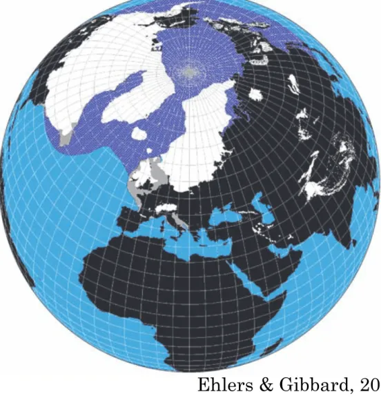
Figure 2 The maximum extent of the Northern Hemisphere LGM ice sheets (from Ehlers and Gibbard, 2004) and the approximate extent of over 0.5 months annual sea-ice cover at the LGM.
Ehlers & Gibbard, 2008
•
Quaternary glacial/interglacial
cycles
•
Largely responsible for current
species distribution
•
Last Glacial Maximum
•
26,000 – 19,000 years BP
•
Ice sheets = maximum extent
Introduction
sequently a substantial ice-dammed lake again formed in the basin during this advance (Busschers, 2008).
The Samarovo glacial maximum of West Siberia is considered to be of Saalian age. However, considering the scarcity of geological information from this region, a pre-Holsteinian glaciation may well have been the most extensive in eastern Central Siberia. During the glacial maximum all northward flowing rivers were blocked, and drainage of Siberia from as far east as Lake Baikal was redirected via the Aral Sea and Caspian Sea into the Black Sea and Mediterranean, multiplying its freshwater supply. Immediately west of the Urals, the position of the ice limits is still controversial. The Saalian limit was probably positioned in the Volga-Pechora interfluve area (Ehlers et al., 2004a).
At the end of the Saalian glacial maximum the ice in Denmark and North Germany possibly melted back beyond the southern Baltic Sea coast. Later readvances in Denmark and North Germany are probably the equivalents of the Warthe (Warta) Substage. Also, the Moscow Till of Russia is the equivalent of the Polish Warta Glaciation. Towards the east, its outer limit converges with that of the Older Saalian (Dnieper) glaciation, and it may even have advanced beyond the Dnieper glacial limit.
In the Alps, the classical Günz comprises several glaciations. Part of what has been originally refererd as Günz is Early Pleisto-cene, part is Middle Pleistocene. Between the Günzian and the Min-delian a separate Haslach Glaciation has been postulated, based on the occurrence of distinct gravel units south of Ulm (Schreiner, 1997). However, the scarcity of early Middle Pleistocene deposits and the lack of age control make it difficult to revise this part of the classical Alpine stratigraphy. Even the stratigraphy of the Alpine Rissian cold Stage is still far from solved—at least in major parts of the glaciated area. Neither the precise extent of the glaciers, nor the number of ice advances or their age, can yet be determined with cer-tainty (Fiebig and Preusser, 2003).
The Middle Pleistocene saw glaciations on many other high mountains, such as, for instance, in Greece (Hughes et al., 2007).
Late Pleistocene and Holocene
(0.13 Ma to present, MIS 1–MIS
5)
In Australia and New Zealand the Last Glacial Maxi-mum occurred towards the end of the Last Glaciation, shortly after 20,000 BP (MIS 2; Suggate, 2004; Col-houn, 2004). The same seems to be true for South America and the High Mountains of Africa (see vari-ous contributions in Ehlers and Gibbard, 2004c). In some regions, however, indications of earlier ice advances during the Last Glaciation have also been found, that might have occurred at MIS 5d or 4.
In North America the extent of Early and Middle Wisconsinan ice is not known. The best information is available for the Last Glacial Maximum, the Late Wisconsinan glaciation. It is now clear, that no ice-free corridor existed between the Cordilleran and the Laurentide Ice Sheet. Based on numerous radiocarbon dates, the North American deglaciation history has been mapped to great detail. The Laurentide Ice Sheet reached its maximum position at about 22 ka B.P., well in advance of the Cordilleran Ice Sheet. It took until 18 ka B.P. before the Wisconsinan ice sheets all over North America had reached their maximum (Dyke, 2004; Andrews and Dyke, 2007).
The extent of Pleistocene glaciation in Highland Asia is still a matter of debate. Kuhle’s (1989) idea that the Tibetan Plateau was covered by a thick ice sheet has been refuted by other workers (Lehmkuhl and Owen, 2005). All authors agree that the Equilibrium-Line Altitudes in parts of Highland Asia were lowered by over 1000 m (Kuhle, 2004; Owen, 2007), and that glaciers were more extensive in the past, but how far this former glaciation reached is still a matter of debate. The inter-pretations rely heavily on the reliability of cosmogenic exposure dat-ing.
In the 1970s through the widespread use of remote sensing data many push moraines were detected in the West Siberian and Pechora
June 2008 214
Table 3 Occurrence of glaciation in the rest of the world through the Cenozoic based on observations presented in contributions to the INQUA project ‚Extent and Chronology of Quaternary Glaciations’ (Ehlers and Gibbard, 2004). Purple squares = glacial deposits; ? = possible glacial deposits; ~ = glaciomarine sediment; MIS = Marine Isotope Stage.
Figure 2 The maximum extent of the Northern Hemisphere LGM ice sheets (from Ehlers and Gibbard, 2004) and the approximate extent of over 0.5 months annual sea-ice cover at the LGM.
•
Quaternary glacial/interglacial
cycles
•
Largely responsible for current
species distribution
•
Last Glacial Maximum
•
26,000 – 19,000 years BP
•
Ice sheets = maximum extent
Ehlers & Gibbard, 2008
Introduction
Cold-adapted taxa demographic hypotheses
•
Cold-adapted taxa
•
Tabula rasa hypothesis
•
Species expand in lowland
areas
•
Nunatak hypothesis
•
Southern mountains nunatak
hypothesis
Hughes et al., 2015
Northern Europe
LGM ice sheet
Introduction
Cold-adapted taxa demographic hypotheses
•
Cold-adapted taxa
•
Tabula rasa hypothesis
•
Nunatak hypothesis
•
Lowland areas too dry
•
Micro-refugia within the
ice-sheets
•
Southern mountains nunatak
hypothesis
Eidesen et al., 2013
Introduction
Cold-adapted taxa demographic hypotheses
•
Cold-adapted taxa
•
Tabula rasa hypothesis
•
Nunatak hypothesis
•
Southern mountains nunatak
hypothesis
•
Micro-refugia only in the
southern mountains
•
Northern area back-colonized
from them
Eidesen et al., 2013
Introduction
Quaternary Refugia
Glacials
Glacials (temperate taxa)
Interglacials
(cold-adapted taxa)
Temperate taxa demographic hypotheses
•
Temperate taxa : refugia
•
Southern refugia hypothesis
•
Northern micro-refugia hypothesis
Stewart & Dalén,
2007
Introduction
Quaternary Refugia
Glacials
Interglacials
(cold-adapted taxa)
Glacials
(temperate taxa)
Temperate taxa demographic hypotheses
•
Temperate taxa : refugia
•
Southern refugia hypothesis
•
Northern micro-refugia hypothesis
•
Predicted from life traits
(Bhagwat & Willis 2008)
•
Short generation time
•
Small seed sizes
•
Reproduce under harsh
conditions
Stewart & Dalén, 2007
Quaternary Refugia
Glacials
Glacials (temperate taxa)
Interglacials
(cold-adapted taxa)
Stewart & Dalén,
2007
Introduction
•
Bryophytes
High cold tolerance
Survive in ice and regenerate after 100’s
to 1000’s of years
→ Good candidates for the nunatak
and the northern micro-refugia hypotheses
High dispersal capacities
Scarcity of the fossil records
La Farge et al., 2013
10cm
Stenoien et al., 2011
Introduction
•
Bryophytes
High cold tolerance
High dispersal capacities
Ability to cross oceans
→ Good candidates for an
extra-European post-glacial recolonization
hypothesis
→ Current dispersal patterns do not
reflect demographic histories
Scarcity of the fossil records
North America
Sphagnum angermanicum:
Introduction
•
Bryophytes
High cold tolerance
High dispersal capacities
Ability to cross oceans
→ Good candidates for an
extra-European post-glacial recolonization
hypothesis
→ Current dispersal patterns do not
reflect demographic histories
Scarcity of the fossil records
10cm
Stenoien et al., 2011
North America
Sphagnum angermanicum:
Introduction
•
Bryophytes
High cold tolerance
High dispersal capacities
→ Current dispersal patterns do not
reflect demographic histories
Scarcity of the fossil records
→ Need for molecular
phylogeography analyses
→ Compare demographic
scenarios
→ Approximate Bayesian
Computation (ABCtoolbox2.0,
including fastsimcoal2)
ABC in a nutshell
1.
Simulation of alleles genealogies
Coalescence technique
Through definition of prior range of values of demographic parameters
Effective population size (Ne)
Migration rate (m)
Scenario 1
Scenario 2
Ne
m
Ne
m
X 10
6X 10
6Scenario 3
Ne
m
X 10
6ABC in a nutshell
2.
Matrices of sequences simulation
Simulation of nucleotide matrices along each of the demographic genealogies
using substitution models
I
1= CAGATCCCAA ... TATGAGCCAT
I
2= ACGACGAAAG ... CATGAGACAG
. . .I
n= CCAAACGATC ... ATGTGCGTGC
locus 1 … locus z
Matrices of simulated sequences
X n scenarios
Model of
sequence
evolution
X 10
6X 10
6ABC in a nutshell
3.
Selection of the best-fit scenario
Describe observed and simulated matrices with summary statistics
Determine the posterior probability of each scenario through an ABC-GLM
approcah
Identify the best-fit scenario
Compute posterior distribution of values
for each parameter
Sc.1
Sc.2
…
Sc.4/6
PP
0.001
0.95
…
0.02
Best-Fit scenario
Sc.1
Sc.2
Sc.3
Sc.4
Material & methods
Cold-adapted taxa
Temperate taxa
= extra-European range
= northern range iced at LGM
= southern mountain range iced at LGM
= southern mountain range ice-free at LGM
= lowland range
= extra-European range
= northern range
= southern range
•
3 species
•
12 species
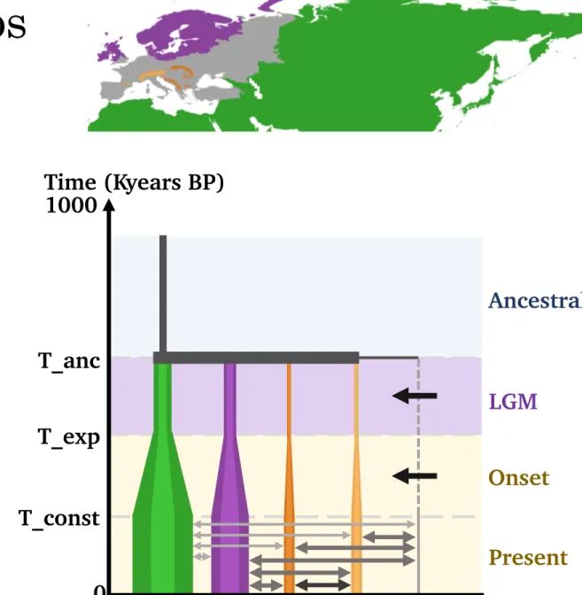
Demographic scenarios
Cold-adapted taxa
•
Nunatak / micro-refugia
•
Present
Population sizes stable
Migrations with
extra-Europe
Migrations between European
populations
•
Onset
Progressive bottleneck in all
populations
•
LGM
Population sizes stable
Figure 6a
Onset
T_const
T_exp
T_anc
1000
Time (Kyears BP)
A1
LGM
Ancestral
0
1
2a
2b
3
0
Present
Onset
T_const
T_exp
T_anc
1000
Time (Kyears BP)
A2
LGM
Ancestral
0
1
2a
2b
3
0
Present
Onset
T_const
T_exp
T_anc
1000
Time (Kyears BP)
A3
LGM
Ancestral
0
1
2a
2b
3
0
Present
Onset
T_const
T_exp
T_anc
1000
Time (Kyears BP)
A4
LGM
Ancestral
0
1
2a
2b
3
0
Present
Onset
T_const
T_exp
T_anc
1000
Time (Kyears BP)
A5
LGM
Ancestral
0
1
2a
2b
3
0
Present
Onset
T_const
T_exp
T_anc
1000
Time (Kyears BP)
A6
LGM
Ancestral
0
1
2a
2b
3
0
Present
Demographic scenarios
Cold-adapted taxa
•
Southern mountains nunatak
hypothesis
•
LGM
Colonization of
N
from ice-free/iced
southern mountains
Figure 6a
Onset
T_const
T_exp
T_anc
1000
Time (Kyears BP)
A1
LGM
Ancestral
0
1
2a
2b
3
0
Present
Onset
T_const
T_exp
T_anc
1000
Time (Kyears BP)
A2
LGM
Ancestral
0
1
2a
2b
3
0
Present
Onset
T_const
T_exp
T_anc
1000
Time (Kyears BP)
A3
LGM
Ancestral
0
1
2a
2b
3
0
Present
Onset
T_const
T_exp
T_anc
1000
Time (Kyears BP)
A4
LGM
Ancestral
0
1
2a
2b
3
0
Present
Onset
T_const
T_exp
T_anc
1000
Time (Kyears BP)
A5
LGM
Ancestral
0
1
2a
2b
3
0
Present
Onset
T_const
T_exp
T_anc
1000
Time (Kyears BP)
A6
LGM
Ancestral
0
1
2a
2b
3
0
Present
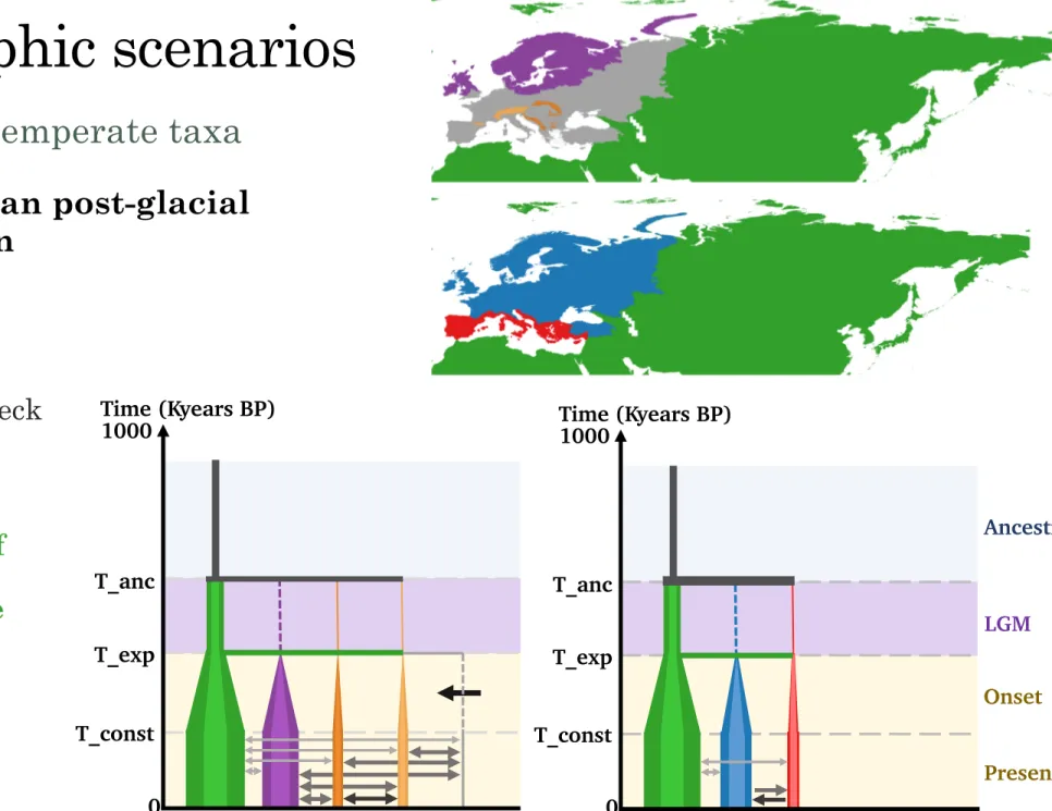
Demographic scenarios
Cold-adapted taxa
•
Tabula rasa
•
Onset
Progressive bottleneck in all
populations
Expansion in
Lowland
•
LGM
Colonization of Europe
from Lowland
Demographic scenarios
Cold-adapted/Temperate taxa
•
Extra-European post-glacial
recolonization
•
Onset
Strong bottleneck
in Europe
•
LGM
Colonization of
Europe from
extra-Europe
Potential
micro-refugia
in Europe
Figure 6a
Onset T_const T_exp T_anc 1000 Time (Kyears BP) A1 LGM Ancestral 0 1 2a 2b 3 0 Present Onset T_const T_exp T_anc 1000 Time (Kyears BP) A2 LGM Ancestral 0 1 2a 2b 3 0 Present Onset T_const T_exp T_anc 1000 Time (Kyears BP) A3 LGM Ancestral 0 1 2a 2b 3 0 Present Onset T_const T_exp T_anc 1000 Time (Kyears BP) A4 LGM Ancestral 0 1 2a 2b 3 0 Present Onset T_const T_exp T_anc 1000 Time (Kyears BP) A5 LGM Ancestral 0 1 2a 2b 3 0 Present Onset T_const T_exp T_anc 1000 Time (Kyears BP) A6 LGM Ancestral 0 1 2a 2b 3 0 PresentFigure 6b
Onset T_const T_exp T_anc 1000 Time (Kyears BP) T1 LGM Ancestral 0 1 2 0 Present Onset T_const T_exp T_anc 1000 Time (Kyears BP) T2 LGM Ancestral 0 1 2 0 Present Onset T_const T_exp T_anc 1000 Time (Kyears BP) T3 LGM Ancestral 0 1 2 0 Present Onset T_const T_exp T_anc 1000 Time (Kyears BP) T4 LGM Ancestral 0 1 2 0 Present T_anc= 26.000-1.000.000 yBP T_exp= 11.000-19.000 yBP T_const=5-11.000 yBP = prior range of effectivepopulation size = migration matrix M1 = migration matrix M2 = migration matrix M12 = migration matrix M21 = migration matrix M3 = migration matrix M4 = migration matrix M5 = glacial period = interglacial period
Fig. 1. Graphical abstract of the integrative method employed to reconstruct the post9glacial history of European bryophytes. (1) Sampling of specimens across their distribution range. (2) Genotyping by Sanger sequencing at selected loci, producing a matrix of observed sequence data. (3) Simulation of sequence data under competing post9glacial recolonization scenarios (3.1). Coalescence simulations are used to generate millions of allele genealogies based on variation in demographic parameters, sampled from prior statistical distributions. One such demographic parameters, population size, is estimated from species distribution models. Matrices of the same size as matrices of observed data are simulated by mapping substitutions on the demographic genealogies using DNA substitution models (3.2). The matrix of observed data and the matrices of simulated data are summarized using summary statistics of populations genetics describing the genetic structure and diversity. The distance between the observed summary statistics and each of the simulated summary statistics are computed and ranked to identify the best9fit scenario showing the shortest distance between observed and simulated data. Posterior statistical distributions of all demographic parameters are then computed from the 1000 shortest simulations from the best9fit scenario.
Figure 6b
Onset
T_const
T_exp
T_anc
1000
Time (Kyears BP)
T1
LGM
Ancestral
0
1
2
0
Present
Onset
T_const
T_exp
T_anc
1000
Time (Kyears BP)
T2
LGM
Ancestral
0
1
2
0
Present
Onset
T_const
T_exp
T_anc
1000
Time (Kyears BP)
T3
LGM
Ancestral
0
1
2
0
Present
Onset
T_const
T_exp
T_anc
1000
Time (Kyears BP)
T4
LGM
Ancestral
0
1
2
0
Present
T_anc= 26.000-1.000.000 yBP T_exp= 11.000-19.000 yBP T_const=5-11.000 yBP = prior range of effectivepopulation size = migration matrix M1 = migration matrix M2 = migration matrix M12 = migration matrix M21 = migration matrix M3 = migration matrix M4 = migration matrix M5 = glacial period = interglacial period
Fig. 1. Graphical abstract of the integrative method employed to reconstruct the post9glacial history of European bryophytes. (1)
Sampling of specimens across their distribution range. (2) Genotyping by Sanger sequencing at selected loci, producing a matrix
of observed sequence data. (3) Simulation of sequence data under competing post9glacial recolonization scenarios (3.1).
Coalescence simulations are used to generate millions of allele genealogies based on variation in demographic parameters,
sampled from prior statistical distributions. One such demographic parameters, population size, is estimated from species
distribution models. Matrices of the same size as matrices of observed data are simulated by mapping substitutions on the
demographic genealogies using DNA substitution models (3.2). The matrix of observed data and the matrices of simulated data
are summarized using summary statistics of populations genetics describing the genetic structure and diversity. The distance
between the observed summary statistics and each of the simulated summary statistics are computed and ranked to identify the
best9fit scenario showing the shortest distance between observed and simulated data. Posterior statistical distributions of all
demographic parameters are then computed from the 1000 shortest simulations from the best9fit scenario.
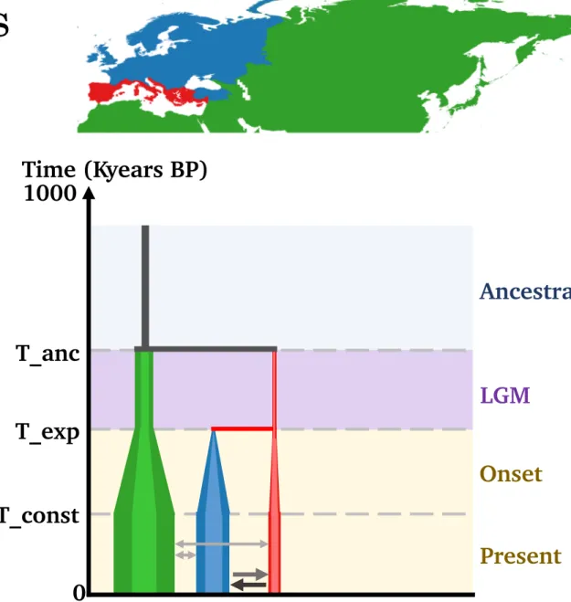
Demographic scenarios
Temperate taxa
•
Southern refugia
•
Onset
Strong bottleneck in
N
•
LGM
Colonization of
N
from S
Figure 6b
Onset
T_const
T_exp
T_anc
1000
Time (Kyears BP)
T1
LGM
Ancestral
0
1
2
0
Present
Onset
T_const
T_exp
T_anc
1000
Time (Kyears BP)
T2
LGM
Ancestral
0
1
2
0
Present
Onset
T_const
T_exp
T_anc
1000
Time (Kyears BP)
T3
LGM
Ancestral
0
1
2
0
Present
Onset
T_const
T_exp
T_anc
1000
Time (Kyears BP)
T4
LGM
Ancestral
0
1
2
0
Present
T_anc= 26.000-1.000.000 yBP T_exp= 11.000-19.000 yBP T_const=5-11.000 yBP = prior range of effectivepopulation size = migration matrix M1 = migration matrix M2 = migration matrix M12 = migration matrix M21 = migration matrix M3 = migration matrix M4 = migration matrix M5 = glacial period = interglacial period
Fig. 1. Graphical abstract of the integrative method employed to reconstruct the post9glacial history of European bryophytes. (1)
Sampling of specimens across their distribution range. (2) Genotyping by Sanger sequencing at selected loci, producing a matrix
of observed sequence data. (3) Simulation of sequence data under competing post9glacial recolonization scenarios (3.1).
Coalescence simulations are used to generate millions of allele genealogies based on variation in demographic parameters,
sampled from prior statistical distributions. One such demographic parameters, population size, is estimated from species
distribution models. Matrices of the same size as matrices of observed data are simulated by mapping substitutions on the
demographic genealogies using DNA substitution models (3.2). The matrix of observed data and the matrices of simulated data
are summarized using summary statistics of populations genetics describing the genetic structure and diversity. The distance
between the observed summary statistics and each of the simulated summary statistics are computed and ranked to identify the
best9fit scenario showing the shortest distance between observed and simulated data. Posterior statistical distributions of all
demographic parameters are then computed from the 1000 shortest simulations from the best9fit scenario.
Demographic scenarios
Temperate taxa
•
Northern micro-refugia
•
Onset
Progressive bottleneck in all
Results
Cold-adapted taxa
•
Best-fit scenarios
•
Expected
Nunatak/Micro-refugia : 2/3 species
•
Classical
Results
Temperate taxa
•
Best-fit scenarios
•
Expected
Northern micro-refugia : 2/12 species
✗
•
Classical
Southern refugia : 3/12 species
✗
Extra-European post-glacial
recolonization : 7/12 species
Posterior distribution : > 90% of
extra-European migrants
Cold-adapted taxa
•
Best-fit scenarios
•
Expected
Nunatak/Micro-refugia : 2/3 species
✓
•
Classical
Results
Temperate taxa
•
Best-fit scenarios
Northern micro-refugia : 2/12 species
✗
Southern refugia : 3/12 species
✗
Extra-European post-glacial
recolonization : 7/12 species
✓
Posterior distribution : > 90% of
extra-European migrants
Results
> 90%
< 10%
Temperate taxa
•
Best-fit scenarios
Northern micro-refugia : 2/12 species
Southern refugia : 3/12 species
Extra-European post-glacial
recolonization : 7/12 species
Posterior distribution : > 90% of
extra-European migrants
0.80 0.85 0.90 0.95 1.00 2.5 3.0 3.5 4.0 4.5 5.0 5.5 CONTRI Density 0 500 1000 1500 2000 2e − 04 3e − 04 4e − 04 5e − 04 T_CONST Density 2500 3000 3500 2e − 04 4e − 04 6e − 04 8e − 04 T_EXP Density 0.00 0.02 0.04 0.06 0.08 0.10 0 5 10 15 20 migRateOUT Density 0.00 0.02 0.04 0.06 0.08 0.10 2 4 6 8 10 12 14 migRateNS Density 0.00 0.02 0.04 0.06 0.08 0.10 2 4 6 8 10 12 14 migRateSN Density 0.80 0.85 0.90 0.95 1.00 2.5 3.0 3.5 4.0 4.5 5.0 5.5 6.0 CONTRI Density 0 500 1000 1500 2000 2e − 04 3e − 04 4e − 04 5e − 04 6e − 04 T_CONST Density 2500 3000 3500 4e − 04 5e − 04 6e − 04 7e − 04 T_EXP Density 0.00 0.02 0.04 0.06 0.08 0.10 0 5 10 15 20 25 migRateOUT Density 0.00 0.02 0.04 0.06 0.08 0.10 2 4 6 8 10 12 14 migRateNS Density 0.00 0.02 0.04 0.06 0.08 0.10 4 6 8 10 12 14 migRateSN Density 0 500 1000 1500 2000 0.000 0.001 0.002 0.003 0.004 T_CONST Density 2500 3000 3500 0.000 0.002 0.004 0.006 0.008 T_EXP Density 0.00 0.02 0.04 0.06 0.08 0.10 0 20 40 60 80 100 120 migRateOUT Density 0.00 0.02 0.04 0.06 0.08 0.10 0 10 20 30 40 50 60 migRateNS Density 0.00 0.02 0.04 0.06 0.08 0.10 0 20 40 60 80 migRateSN Density 0 500 1000 1500 2000 0e+00 2e − 04 4e − 04 6e − 04 8e − 04 1e − 03 T_CONST Density 2500 3000 3500 3e − 04 4e − 04 5e − 04 6e − 04 7e − 04 8e − 04 T_EXP Density 0.00 0.02 0.04 0.06 0.08 0.10 0 5 10 15 20 25 migRateOUT Density 0.00 0.02 0.04 0.06 0.08 0.10 5 10 15 migRateNS Density 0.00 0.02 0.04 0.06 0.08 0.10 6 8 10 12 migRateSN DensityM
et
zge
ri
a
conj
ugat
a
M
et
zge
ri
a
fur
cat
a
O
rt
hot
ri
chum
af
fi
ne
O
rt
hot
ri
chum
ly
ellii
0e+00 1e+06 2e+06 3e+06 4e+06 5e+06
1.0e − 07 1.2e − 07 1.4e − 07 1.6e − 07 1.8e − 07 2.0e − 07 2.2e − 07 NORTH_PRESENT Density
0.0e+00 5.0e+06 1.0e+07 1.5e+07
4e − 08 5e − 08 6e − 08 7e − 08 8e − 08 OUT_PRESENT Density
0e+00 2e+05 4e+05 6e+05 8e+05 1e+06
5.0e − 07 7.0e − 07 9.0e − 07 1.1e − 06 SOUTH_PRESENT Density
0e+00 2e+06 4e+06 6e+06 8e+06 1e+07
5.0e − 08 7.0e − 08 9.0e − 08 1.1e − 07 NORTH_PRESENT Density
0.0e+00 5.0e+06 1.0e+07 1.5e+07
3e − 08 4e − 08 5e − 08 6e − 08 OUT_PRESENT Density 0 500000 1000000 2000000 3000000 1.5e − 07 2.0e − 07 2.5e − 07 3.0e − 07 SOUTH_PRESENT Density 0 20 40 60 80 100 0.00 0.02 0.04 0.06 0.08 0.10 0.12 NORTH_LGM Density
0e+00 2e+06 4e+06 6e+06 8e+06
0e+00 2e − 07 4e − 07 6e − 07 8e − 07 1e − 06 NORTH_PRESENT Density
0.0e+00 2.0e+06 4.0e+06 6.0e+06 8.0e+06 1.0e+07 1.2e+07 1.4e+07
0e+00 2e − 07 4e − 07 6e − 07 8e − 07 OUT_PRESENT Density 0 500000 1000000 1500000 2000000 2500000 3000000 0.0e+00 5.0e − 07 1.0e − 06 1.5e − 06 2.0e − 06 2.5e − 06 SOUTH_PRESENT Density
0e+00 2e+06 4e+06 6e+06 8e+06 1e+07
4.0e − 08 6.0e − 08 8.0e − 08 1.0e − 07 1.2e − 07 NORTH_PRESENT Density
0.0e+00 5.0e+06 1.0e+07 1.5e+07 2.0e+07
3e − 08 4e − 08 5e − 08 6e − 08 7e − 08 OUT_PRESENT Density
0e+00 1e+06 2e+06 3e+06 4e+06
1.0e − 07 1.5e − 07 2.0e − 07 2.5e − 07 3.0e − 07 SOUTH_PRESENT Density